Article

Modeling of Tensile Stress Distribution Considering Anisotropy of Mechanical Properties of Thin-Walled AlSi10Mg Samples Obtained by Selective Laser Melting

1
Spark Plasma Sintering Research Laboratory, Moscow State University of Technology “STANKIN”, Vadkovsky per. 1, 127055 Moscow, Russia
2
College of New Materials and Nanotechnologies, National University of Science & Technology (MISIS), Leninskii prosp, 4, 119049 Moscow, Russia
3
Laboratory of Innovative Additive Technologies, Moscow State University of Technology “STANKIN”, Vadkovsky per. 1, 127055 Moscow, Russia
4
Scientific Department, Federal State Budgetary Educational Institution of Higher Education, “Russian University of Medicine” of the Ministry of Health of the Russian Federation, Dolgorukovskaya Str. 4, 127006 Moscow, Russia
*
Author to whom correspondence should be addressed.
J. Manuf. Mater. Process. 2024, 8(5), 235; https://doi.org/10.3390/jmmp8050235
Submission received: 20 August 2024 / Revised: 1 October 2024 / Accepted: 17 October 2024 / Published: 20 October 2024

Abstract

:
The work that is being presented demonstrates that there is a critical point at which the engineering stress–strain diagram’s elastic–plastic region transitions to yield and fracture stresses. This transition is demonstrated using thin-walled specimens made using selective laser melting technology from high-strength aluminum alloys (AlSi10Mg) that have undergone preliminary heat treatment. It was discovered that the strain-hardening coefficient, which was determined in the section from yield strength to fracture strength, and the critical point have a highly statistically significant association (0.83 by Spearman and 0.93 by Pearson). It was possible to derive a regression equation that connected the strain-hardening coefficient with the crucial transition point. The type of stress distribution in the elastic–plastic region changes (the Weibull distribution changes to a normal distribution) as the plasticity of the thin-walled samples increases. Additionally, the contribution of the probability density of the stress distribution described by the Cauchy distribution increases in a mode near the point at which the probability density of the fracture increases.

1. Introduction

Precise modeling of the material fracture process is necessary for complex product design. By optimizing the final product’s design based on actual loads, modeling aims to increase the structure’s reliability.
The mathematical (numerical methods) foundation for engineering computations is provided by various iterations of the mesh method [1] and the finite volume approach [2], while the physical foundation is provided by continuum mechanics [3]. This application of elasticity theory demonstrates well the fracture of samples made from acrylonitrile butadiene styrene (ABS) plastic and composite materials using fused deposition modeling (FDM) technology [4,5,6]. Similar examples are available for calculating strength and modeling the selective laser melting process [7,8,9]. Many materials, especially composite materials, have heterogeneous mechanical properties [10,11,12,13,14,15,16,17,18], which makes it necessary to assess the dependability of almost all structural materials using a probabilistic method [19].
The most popular distribution for the probabilistic modeling of structural material reliability is the two-parameter Weibull distribution [20,21]. The Weibull distribution was utilized in [22] to estimate the size distribution of fiber inclusions, in a manner like how it is used in studies on other materials, such as composite materials [6,22]. Weibull did note in his publications that the Weibull distribution should be considered an empirical distribution in addition to other distribution functions [20,21].
So, using the Akaike information criterion [23], a novel approach to evaluating the kind of distribution of mechanical features was proposed [24]. This demonstrated that the normal distribution is the closest type of stress distribution for certain materials (silicon oxide). Using the Akaike and Bayes criteria, it was demonstrated that the logistic distribution is the closest type of distribution for the mechanical properties of pipe steels [18]. An investigation of mechanical properties in terms of the tension of samples generated from high-strength aluminum alloy (AlSi10Mg) using selective laser melting technology and applying the Akaike and Bayes information criteria shows that the Weibull distribution is the closest [25].
As shown in [26], the Cauchy distribution is the closest distribution to the Weibull distribution for the particle size distribution of alumina (Al2O3) inclusions in polylactic acid (PLA). Furthermore, it was shown that different sections of the same FDM-printed sample and different regions of the same filament containing Al2O3 inclusions may exhibit different distribution rules for the dispersion of ceramic inclusions in plastic.
There exists a clear correlation between the homogeneity of inclusion distribution and the mechanical properties of samples fabricated using selective laser melting (SLM) and composite materials [26]. In the second case, the achieved strengthening results from the distribution of various inclusions that precipitate along the phase boundary during heat treatment of samples acquired by SLM [27,28,29,30,31,32,33]. In [34,35], it was shown that hardening in AlSi10Mg is achieved due to the ultrathin eutectic microstructure of a spherical nanoscale network of eutectic Si embedded in the Al matrix. In [35], the size distribution of inclusions was investigated, but no attention was paid to the law of particle size distribution and its change depending on heat treatment.
It is controversial to base the understanding of complex multistage processes, like material fracture under tension, on a single type of distribution. Consequently, Bayesian statistics and Markov chain theory are widely applied in the probabilistic modeling of complex systems [36,37], and mixture theory is often applicable [38].
Engineering stress–strain diagrams of filament and printed samples made from ABS, PLA, and ceramic/polylactide acid (60% Al2O3/40% PLA) utilizing FDM technology, as well as the fracture probabilities analysis of pre-cycled samples, were described in [39,40].
Based on an investigation of the behavior of the fracture probability densities with respect to stresses in samples made by selective laser melting, this work proposes an extension of the hypothesis [40].
This work aims to present a model of stress distribution in samples that underwent tensile testing and that were generated by selective laser melting of AlSi10Mg.

2. Materials and Methods

2.1. Materials

Powdered AlSi10Mg was the first material utilized to manufacture the samples utilizing selective laser melting. The sizes of the powders ranged from 30 to 75 µm. Figure 1 [25] shows a micrograph of the initial material and the powder particle size distribution.
Figure 1. (A) SEM picture of the original powdered AlSi10Mg. Distribution of particle sizes (B) The original AlSi10Mg powder’s average chemical composition is shown in Table 1.
Jmmp 08 00235 g001
A 3D metal printer, the FS121M (Farsoon Technologies, Hunan, China), was equipped with a preinstalled 500 W laser. Layer thickness of 30 µm, laser power P = 340 W, hatching distance of 0.15 mm, and laser travel speed of 1500 mm/sec were the primary printing modes. Figure 2 shows a schematic of the sample and where it was placed on the table during the selective laser melting production process.
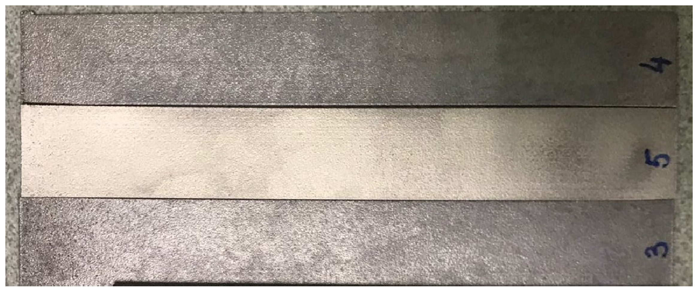
In steps of 30 °C, the printed samples were heat-treated in an air-filled muffle furnace at temperatures between 260 °C and 440 °C. Following an hour of heating to the holding temperature, the samples were allowed to cool naturally at the furnace’s rate. The heat-treated specimens were subjected to mechanical testing and surface roughness analysis. The acquired samples are displayed in Figure 3.
Ref. [25] provides microstructure and technical “stress-strain” diagrams that are based on the test results of the specimens shown in Figure 3.

2.2. Experimental Methods

The microstructure and chemical makeup of the materials were examined using a Phenom ProX scanning electron microscope (Phenom-World BV, Eindhoven, Holland) equipped with an adaptor for elemental analysis by energy-dispersive spectroscopy. The surface roughness of the samples was measured with a Hommel-Etamic T8000 profilometer (Jenoptik, Jena, Germany), and mechanical tensile tests were conducted at a speed of 2 mm/min using an INSTRON 5989 electromechanical testing machine (Instron, Norwood, MA, USA).

2.3. Theoretical Methods

The behavior of fracture probability densities is analyzed to provide a theoretical framework for both the analysis of fracture probability and the processes involved in tensile fracture [21]. In this study, we utilized the methodology initially introduced in [40], specifically applying it to the fracture probability of specimens produced using SLM technology from AlSi10Mg. The experimental data were statistically analyzed using Rstudio 2023.06.1 Posit Software, PBC, GNU license. Using experimental data from [25] and the theory described in [41,42,43,44], the empirical fracture probability density function was computed.
f ^ h σ = 1 n i = 1 n 1 h d i k K ( t σ i h d i k )
where n is the number of points in the stretching diagram; K—is the “kernel” function; k—is an arbitrary positive number; dik is the distance from σi to the k nearest point in the stretching diagram data consisting of n−1 other points; h is the smoothing parameter; and t—is the local point at which the state density function is defined.
Equation (1) indicates that the specimens produced by SLM technology have a continuous fracture probability density function that is defined at all stresses between 0 and σF, where σF is the fracture stress. The fracture probability density function of the specimens acquired by SLM technology can be decomposed in Fourier series based on the continuity requirement of the function f ^ h ( σ ) . The rapid Fourier transform was used in the study that was presented.
ρ γ = i = 1 n f ^ h ( σ i ) e x p ( 2 π i γ , σ i )
where ρ(γ) is the spectral density of tensile stress distribution of SLM specimens; f ^ h ( σ i ) is the probability density of failure of SLM specimens.
According to Euler’s equation, the argument, given f ^ h ( σ i ) and σ i , determines the behavior of the spectral function. It follows from Equation (2) that all values of the spectral density of the stress distribution belong to the space of complex numbers.
γ = R e ( ρ γ ) / I m ( ρ γ )
where γ is the argument of the spectral probability density function; Re(ρ(γ)) is the real part of the spectral probability density function of fracture probability; and Im(ρ(γ)) is the imaginary part of the spectral probability density function of fracture probability.
The following algorithm was used to look for symmetry in the spectral density argument’s behavior:
φ i σ = γ i   a t   d γ d σ = 0
φ i σ + φ i σ T σ = 0
where φ i σ is the value of the argument of the spectral function corresponding to the maximum or minimum of the spectral function; σ T is the voltage value at which the spectral probability density function exhibits symmetry properties.
The behavior of the theoretical probability density function to the left and right of the stress σ T corresponding to Equation (5), symmetry breaking in the vicinity of σ T , and changes in the type of the theoretical distribution to the left and right of σ T are the main areas of interest for the analysis of the empirical fracture probability density function [45].
The determination of the closest theoretical type of simple distribution to the empirical distribution was carried out using the minimum value of Akaike’s criterion and Bayes’ criterion. And the simple theoretical distributions were as follows:
  • Normal:
f σ = 1 s d 2 π e x p ( ( σ μ ) 2 2 s d 2 )
where sd is the mean square deviation of the stresses; μ is the mathematical expectation of the stress distribution; and σ is the stresses.
2.
Logarithmically normal:
f σ = 1 σ × s d × 2 × π exp ln σ μ 2 2 × s d 2
3.
Logistical:
f σ = 1 s × exp σ μ s 1 + exp σ μ s 2
4.
Cauchy:
f σ = 1 π × s × 1 + σ x 0 s 2
where s is the scale factor; x0 is the shift factor.
5.
Weibull:
f σ = a b × σ b ( a 1 ) × exp σ b a
where a is the shape factor of the Weibull distribution; b is the scale factor of the Weibull distribution.
6.
Poisson:
f σ = μ k k ! × e x p ( μ )
where k is the number of events (studies).
7.
Exponential:
f σ = λ × e x p ( λ σ )
where λ = 1/μ is the inverse of the mathematical expectation.
8.
Gumbel:
f σ = e x p ( σ + e x p ( σ )
The parameters of the distributions were calculated using the maximum likelihood method [44,46].
The determination of the total fracture probability density for the bound state of SLM specimens was calculated using the following equation [47]:
f ( σ ) ¯ = i = 1 N f ^ i h σ
where f ^ i h ( σ ) is the fracture probability density of the i-th specimen; N is the number of tested specimens; and f ( σ ) ¯ is the total probability density of fracture for the bound state of SLM specimens.
The calculation of the sample fracture probability density based on the identified theoretical probability densities was performed using the following equation:
f i σ = k = 1 l ω k f k ( σ ) m , j = 1 l f m σ f j σ
where f i ( σ ) is the probability density of failure of the i-th specimen; k is the number of the stress distribution; ω k is the weight of the k-th probability density in the probability density of failure of the specimen; and f k ( σ ) is the probability density of the distribution at the k-th site of the stress distribution.
Theoretical probability density functions were matched with each acquired general probability density distribution function of fracture probability, and the difference (“non-convexity”) between the general probability densities was determined by the following formula:
D f = 1 n + 1 i = 1 n ( f i T σ f i P ( σ ) ) 2 2
where f i T ( σ ) is the average theoretical probability density of stress distribution at static failure; f i P ( σ ) is the actual average probability density of stress distribution at static failure; and n is the number of points in the state density function.
Mechanical property anisotropy can appear from sample to sample [20] as well as within a single sample produced by selective laser melting [48]. In this study, we examined the anisotropy of the material’s mechanical characteristics as they vary among samples in the tensile testing of SLM AlSi10Mg samples with narrow walls.

3. Results and Discussion

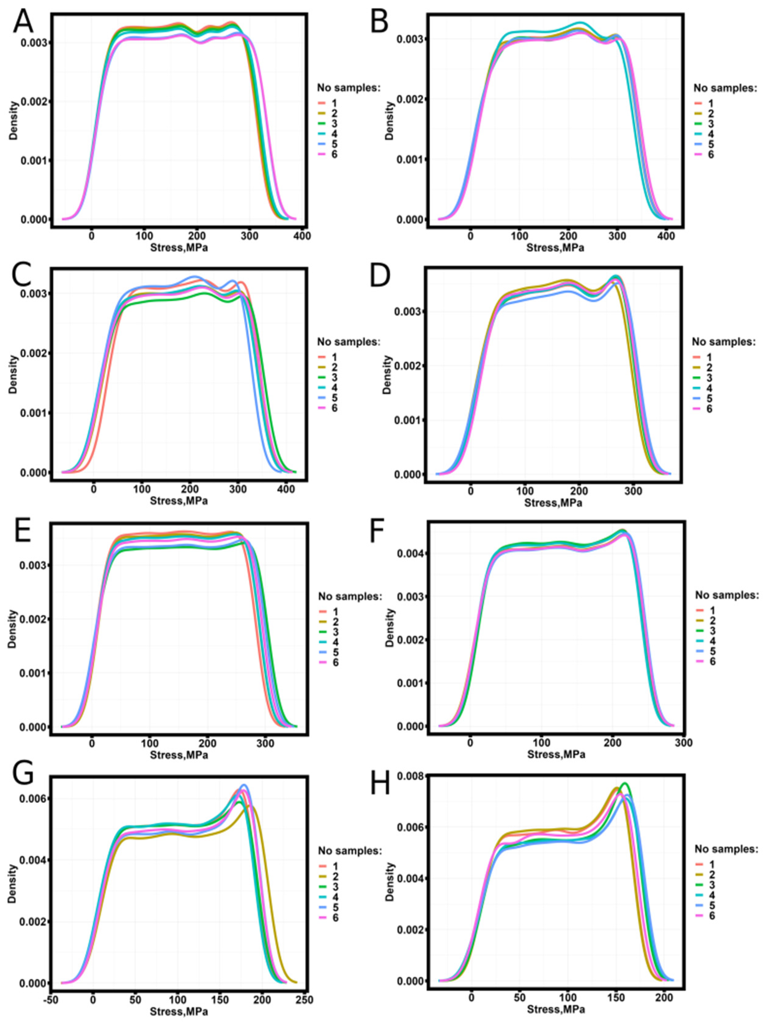
Stress–strain tensile diagrams of specimens fabricated by SLM technology from AlSi10Mg [25] were obtained for a series of static tensile tests. The empirical fracture probability densities calculated by Equation (1) are presented in Figure 4.
In contrast to the behavior of the empirical probability density of filament samples and samples obtained by FDM printing technology from ABS, PLA, and 60% Al2O3/40% PLA, the analysis of the behavior of the empirical probability density of fracture of SLM samples reveals that the empirical probability density of samples prior to heat treatment at 350 °C inclusive (Figure 4A–E) does not have one clearly expressed extremum [38]. The empirical probability density for the SLM samples that were heat-treated at temperatures higher than 350 °C (Figure 4F–H) has a single, prominent maximum, and the contribution to the total fracture probability density increases with the annealing temperature.
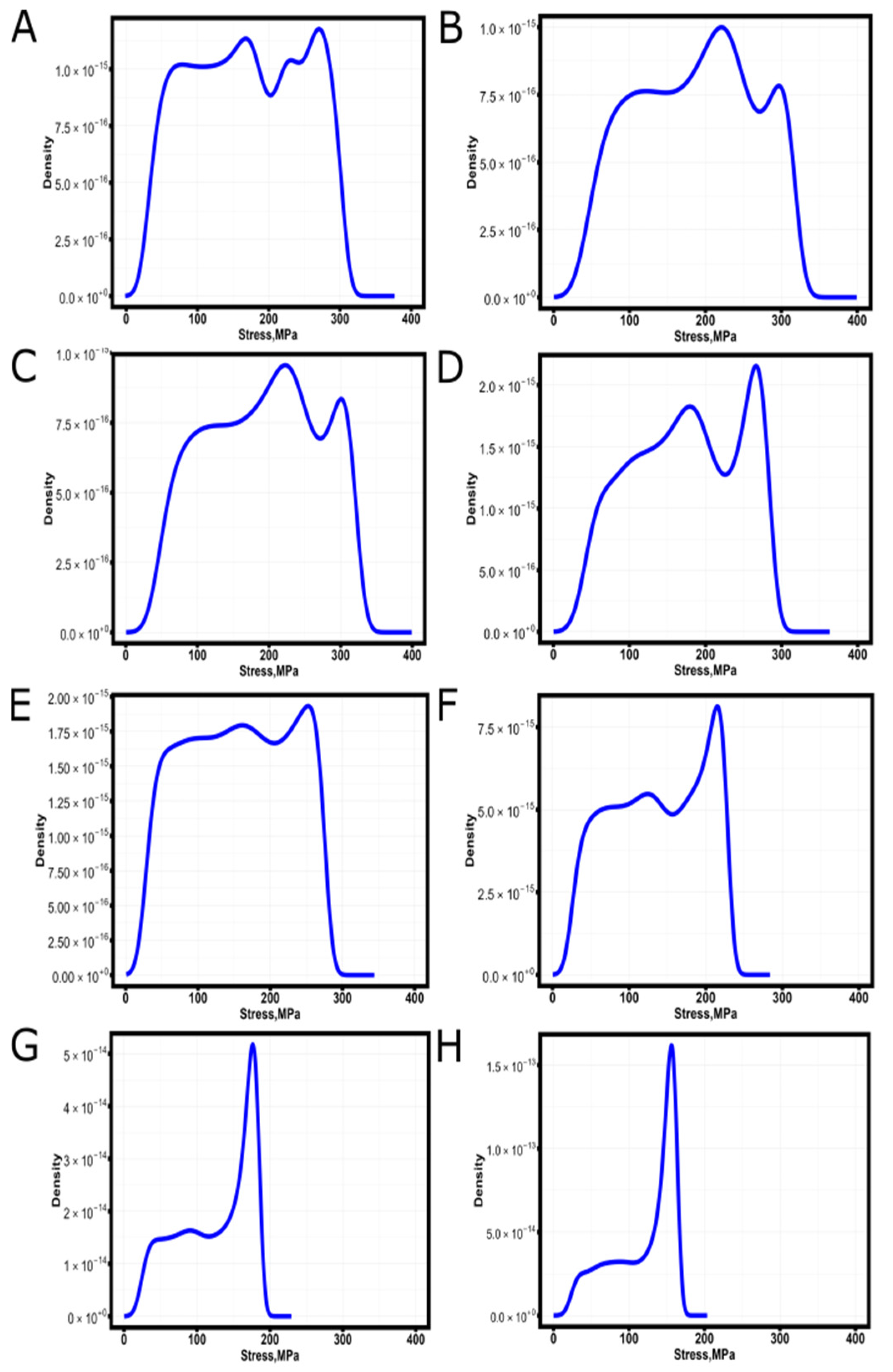
Figure 5 shows the results of calculating the argument (3) of the spectral density (2) of states for the studied samples.
The behavior of the argument of the spectral density function of states from stresses has a break at the symmetry point of the maxima and minima of the argument, and its nature is similar to that of the behavior described in [40].
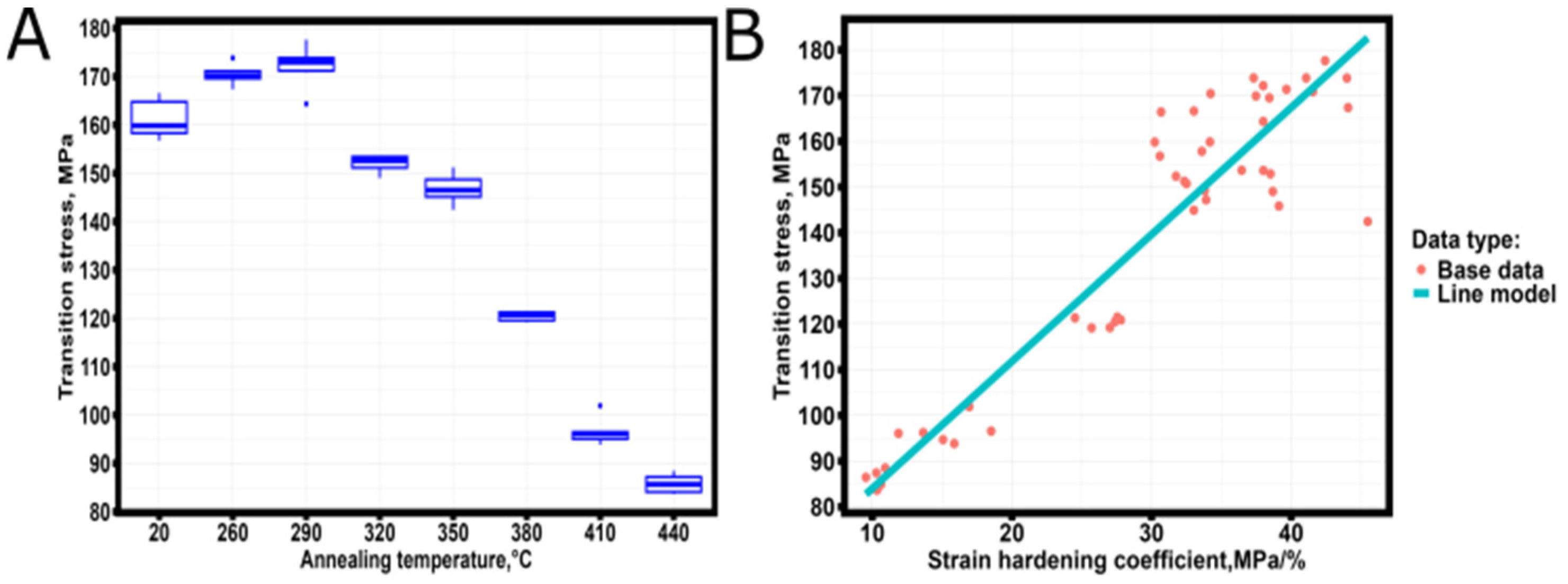
Upon confirming the existence of a Spearman correlation between the strain-hardening coefficient and the transition point values [25], the correlation coefficient value was found to be 0.83 at the statistical significance level, with a p-value of 3.023 × 10⁻¹³, and 0.93 at the level of statistical significance, with a p-value of <2.2 × 10⁻¹⁶. There is a strong statistically significant association between these numbers.
The influences of transition points on the temperature of the heat treatment and the transition points on the strain-hardening coefficient found in [25] are displayed in Figure 6.
The high value of the correlation coefficient indicates a linear relationship between σT and θ (the robotic regression algorithm [49] was used to build a linear model):
σ T = 56.2459 + 2.7786 × θ
The linear model’s mean square deviation from the data is 9.876 MPa. Equation (17) can be represented more broadly as follows: the free term of the equation has the dimension of stress, and the multiplier before the strain-hardening coefficient has the dimension of strain, according to an analysis of the dimensionality [50] of the values included in the equation.
σ T = σ 0 + ε 0 × θ
where σ0 is the stress corresponding to the beginning of the transition from the elastic to plastic region of the strain diagram; ε0 is the strain change at the section of transition from the elastic to fracture region of the engineering stress–strain diagram.
The nearest type of stress distribution to the left and right of σT was studied using the Akaike and Bayes criteria. Among the eight distribution types found in Equations (6)–(13), the distribution with the lowest Akaike and Bayes criteria values was chosen. The maximum likelihood technique [51] was used to compute the parameters of the distribution functions. Table 2 displays the findings of the analysis.
The Weibull distribution scale parameter (b in Equation (10)) and the mathematical expectation (in the case of a normal distribution) increase in absolute value up to the heat treatment temperature of 290 °C and decrease afterward, according to an analysis of the behavior of the Weibull distribution parameters to the left and right of the transition point. There is no similar reliance for the Weibull distribution’s shape parameter (in Equation (10), except situations in which a normal distribution turns out to be the closest type of distribution. The mean square deviation of uniformly distributed stresses increases with the heat treatment temperature. As the heat treatment temperature rises, the features of the stress distribution go to the left of the transition point. The closest type of simple transition stress distribution to the left of the transition point and the annealing temperature were found to have a moderate (almost strong) relationship, as indicated by the value of 0.4733 obtained from applying Kramer’s [52] V criterion to the correlation between the distribution type change and annealing temperature at the section to the left of the transition point. Changes in the structural phase composition of the heat-treated samples can be responsible for the change in the prevailing kind of transition stress distribution to the left of the transition point. The closest type of distribution to the right of the transition point, as determined by the Akaike and Bayes information criteria, did not vary.
To determine the statistical relationship between the mechanical characteristics and distribution coefficients, a Spearman correlation study was conducted. This analysis took into account the overall association and was not temperature-specific. The analysis’ findings are presented in Table 3.
The correlation analysis results indicate that the fundamental mechanical properties of the specimens are strongly correlated with coefficient b (mathematical expectation in the case of a normal distribution) of the Weibull distribution to the left of the transition point, whereas coefficient a (mean square deviation in the case of a normal distribution) is weakly statistically significantly correlated with the deformation corresponding to the ultimate strength.
While coefficient a has a medium statistically significant correlation with the basic mechanical properties of the AlSi10Mg samples, the correlation analysis of the Weibull distribution coefficients to the right of the transition point reveals a strong correlation with the basic mechanical properties of the SLM samples.
The primary regression equations for the discovered statistically significant dependencies are shown in Table 4; the equation parameters were determined using the robust regression algorithm [49].
Further research is needed to confirm or refute the relationship between the coefficients of the distributions (Table 2) and the relative values found from tensile diagrams (hardening coefficient corresponding to different stages of dislocation motion). This relationship is suggested by an analysis of the obtained regression equations.
Equation (14), when applied to the analysis of bound states, reveals that the Cauchy distribution [31], which has a maximum around σD (fracture stress), contributes more as the heat treatment temperature rises. Figure 7 displays the fracture probability density of the bound states for six samples.
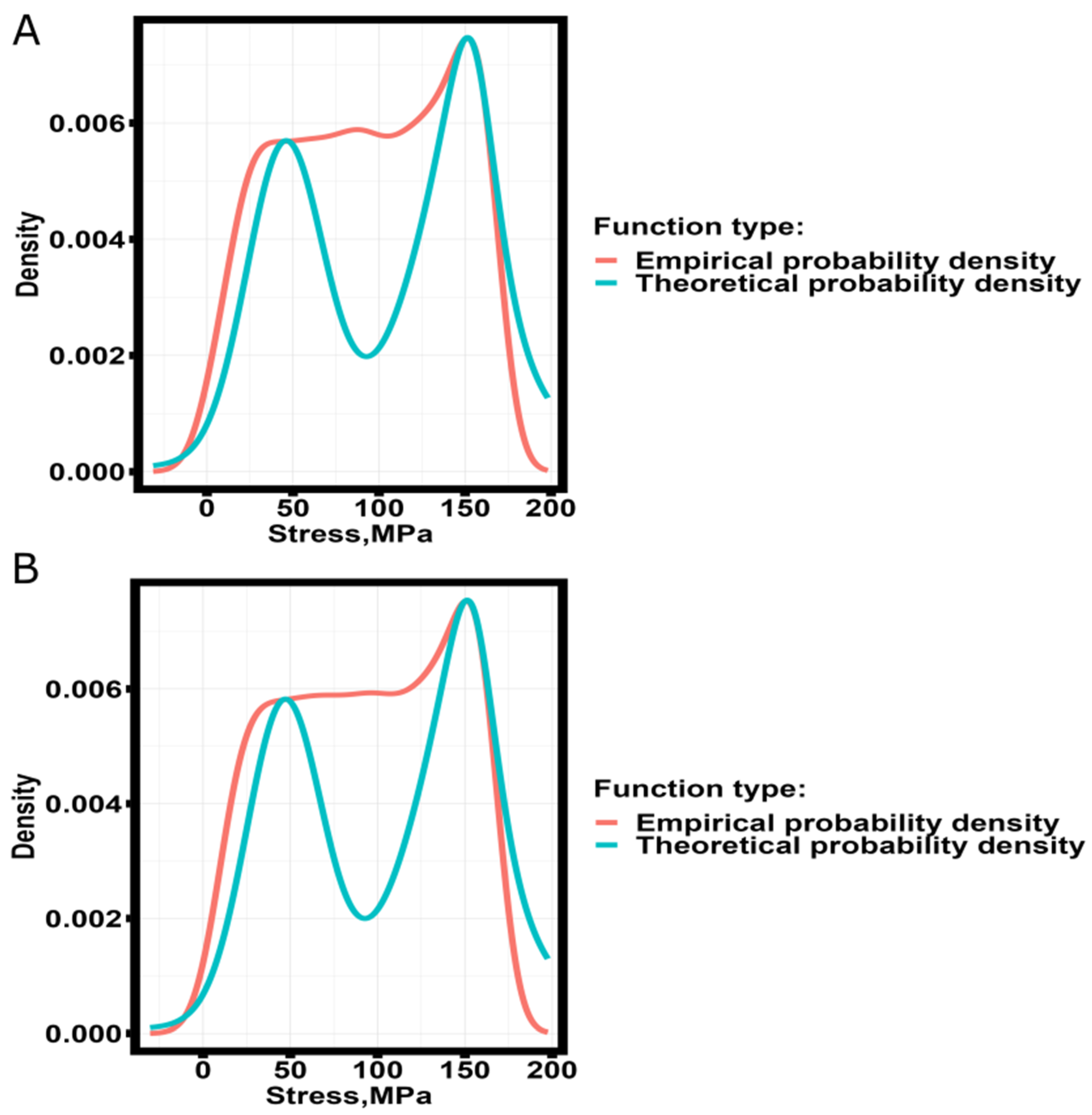
The Cauchy distribution degenerates into the probability density of failure of the bound state, described by a complicated distribution, as the number of bound states of samples heat-treated at 410 °C and 440 °C increases. With the aforementioned in mind, the fracture probability density of the samples produced by selective laser melting of AlSi10Mg has been reconstructed using Equation (15) and the findings of the investigation of stresses to the left and right of the transition point (Table 2). The probability density modeling findings for samples No. 1 and No. 2, which were heat-treated at 440 °C, are displayed in Figure 8.
For SLM samples, the theoretical fracture probability density has more prominent features in the region of the transition point, which calls for additional research to improve the model (15). This is in contrast to the description of the fracture probability density of the filament and samples made by FDM printing technology [40]. The theoretical probability density (16) has very modest levels of divergence from the actual one, even when there are visible anomalies. Table 5 displays the findings of the deviation calculations.
Thus, the approach developed in [31] can be applied to describe the fracture probability of samples obtained by selective laser melting of AlSi10Mg alloy.

4. Conclusions

The strain-hardening coefficient, which is computed based on the section from the yield strength to the strength in the engineering stress–strain diagram, is strongly correlated with the stress value that corresponds to minus infinity of the argument of the spectral function of the density of states (transition stress), according to the analysis. We were able to determine a general relationship between the strain-hardening coefficient, the value of the transition point, and the mechanical properties of the material by the application of robotic regression analysis and the theory of dimensionality.
By utilizing the Akaike and Bayes information criteria, we were able to determine that when the temperature of the sample heat treatment increases, the distribution of stresses to the left of the transition point shifts from a Weibull distribution to a normal distribution. By using Kramer’s criterion, it was discovered that there is a moderately substantial statistical correlation between this change and the heat treatment temperature of samples generated from the AlSi10Mg alloy using the selective laser melting technique. Based on research by other authors, it can be said that structural and phase changes in the material after heat treatment are related to the variation in the closest theoretical stress distribution.
The analysis of the bound states of the specimens revealed that the contribution of the fracture probability density described by the Cauchy distribution with a mode in the fracture stress region of the specimens increases with increasing ductility of the material following heat treatment.
The investigation led to the development of a theoretical model that describes the fracture probability density, and this model fits well with the empirical fracture probability density.
In the appropriate sections of the engineering stress–strain diagrams, more research will be conducted to characterize the change from the Weibull distribution to the normal distribution and to determine the connection between the strain hardening and the coefficients of the theoretical distributions.

Author Contributions

Conceptualization, N.Y.N., A.F. and P.S.; methodology, N.Y.N., A.M. and M.V.; software, N.Y.N., R.K. and I.I.; validation, A.F., P.S. and A.M.; formal analysis, N.Y.N. and M.V.; investigation, R.K.; resources, S.N.G. and P.P.; data curation, I.I.; writing—original draft preparation, N.Y.N.; writing—review and editing, N.Y.N. and S.N.G.; visualization, A.F. and P.S.; supervision, S.N.G.; project administration, P.P.; funding acquisition, S.N.G. and P.P. All authors have read and agreed to the published version of the manuscript.

Funding

The research was supported by the Ministry of Science and Higher Education of the Russian Federation: project FSFS-2023-0003.

Data Availability Statement

The data provided in this study are available upon request from the corresponding author.

Conflicts of Interest

The authors declare no conflicts of interest.

References

  1. Huebner, K.H.; Dewhirst, D.L.; Smith, D.E.; Byrom, T.G. The Finite Element Method for Engineers; John Wiley & Sons: Hoboken, NJ, USA, 2001; ISBN 978-0-471-37078-9. [Google Scholar]
  2. Eymard, R. The finite volume method Handbook of Numerical Analysis. Handb. Numer. Anal. 2000, 7, 713–1020. [Google Scholar]
  3. Atanackovic, T.M.; Guran, A. Theory of Elasticity for Scientists and Engineers; Dover Books on Physics; Springer Science & Business Media: Berlin/Heidelberg, Germany, 16 June 2000; ISBN 978-0-8176-4072-9. [Google Scholar]
  4. Rodríguez, J.F.; Thomas, J.P.; Renaud, J.E. Mechanical behaviour of acrylonitrile butadiene styrene (ABS) fused deposition materials. Experimental investigation. Rapid Prototyp. J. 2001, 7, 148–158. [Google Scholar] [CrossRef]
  5. Grigoriev, S.; Peretyagin, N.; Apelfeld, A.; Smirnov, A.; Morozov, A.; Torskaya, E.; Volosova, M.; Yanushevich, O.; Yarygin, N.; Krikheli, N.; et al. Investigation of Tribological Characteristics of PEO Coatings Formed on Ti6Al4V Titanium Alloy in Electrolytes with Graphene Oxide Additives. Materials 2023, 16, 3928. [Google Scholar] [CrossRef]
  6. Zak, G.; Haberer, M.; Park, C.B.; Benhabib, B. Mechanical properties of short fiber layered composites. Rapid Prototyp. J. 2000, 6, 107–118. [Google Scholar] [CrossRef]
  7. Contuzzi, N.; Campanelli, S.L.; Ludovico, A.D. 3D finite element analysis in the selective laser melting process. Int. J. Simul. Model. 2011, 10, 113–121. [Google Scholar] [CrossRef] [PubMed]
  8. Ahmadi, A.; Moghaddam, N.S.; Elahinia, M.; Karaca, H.E.; Mirzaeifar, R. Finite element modeling of selective laser melting 316L stainless steel parts for evaluating the mechanical properties. In Proceedings of the ASME 2016 11th International Manufacturing Science and Engineering Conference, Blacksburg, VA, USA, 27 June–1 July 2016; American Society of Mechanical Engineers: Richmond, VA, USA, 2016; Volume 49903. [Google Scholar]
  9. Păcurar, R.; Păcurar, A.; Petrilak, A.; Bâlc, N. Finite element analysis to predict the mechanical behavior of lattice structures made by selective laser melting technology. Appl. Mech. Mater. 2014, 657, 231–235. [Google Scholar] [CrossRef]
  10. Lawn, B.R. Fracture of Brittle Solids, 2nd ed.; Cambridge University Press: Cambridge, UK, 1993. [Google Scholar]
  11. Konov, S.; Frolov, A.; Shapovalov, P.; Peretyagin, P.; Grigoriev, S. Segmented Four-Element Photodiodes in a Three-Dimensional Laser Beam Angle Measurement. Photonics 2023, 10, 704. [Google Scholar] [CrossRef]
  12. Herrmann, H.J.; Roux, S. (Eds.) Statistical Models for the Fracture of Disordered Media; Elsevier: Amsterdam, The Netherlands, 1990. [Google Scholar]
  13. Grigoriev, S.; Peretyagin, N.; Apelfeld, A.; Smirnov, A.; Yanushevich, O.; Krikheli, N.; Kramar, O.; Kramar, S.; Peretyagin, P. Investigation of MAO Coatings Characteristics on Titanium Products Obtained by EBM Method Using Additive Manufacturing. Materials 2022, 15, 4535. [Google Scholar] [CrossRef] [PubMed]
  14. Curtin, W.A. Size scaling of strength in heterogeneous materials. Phys. Rev. Lett. 1998, 80, 1445. [Google Scholar] [CrossRef]
  15. Smirnov, A.; Kuznetsova, E.; Pristinskiy, Y.; Podrabinnik, P.; Mironov, A.; Gershman, I.; Peretyagin, P. Effect of Milling Conditions on the Microstructural Design in Aluminum Based Alloy Fabricated by SPS. Metals 2019, 9, 1164. [Google Scholar] [CrossRef]
  16. Kurmysheva, A.Y.; Yanushevich, O.; Krikheli, N.; Kramar, O.; Vedenyapina, M.D.; Podrabinnik, P.; Solís Pinargote, N.W.; Smirnov, A.; Kuznetsova, E.; Malyavin, V.V.; et al. Adsorption Ability of Graphene Aerogel and Reduced Graphene Aerogel toward 2,4-D Herbicide and Salicylic Acid. Gels 2023, 9, 680. [Google Scholar] [CrossRef] [PubMed]
  17. Grigoriev, S.; Peretyagin, N.; Apelfeld, A.; Smirnov, A.; Rybkina, A.; Kameneva, E.; Zheltukhin, A.; Gerasimov, M.; Volosova, M.; Yanushevich, O.; et al. Investigation of the Characteristics of MAO Coatings Formed on Ti6Al4V Titanium Alloy in Electrolytes with Graphene Oxide Additives. J. Compos. Sci. 2023, 7, 142. [Google Scholar] [CrossRef]
  18. Skorodumov, S.V.; Neganov, D.A.; Studenov, E.P.; Poshibaev, P.V.; Nikitin, N.Y. Statistical analysis of mechanical test results for samples of pipes from trunk oil pipelines after long-term operation. Industr. Lab. Diagn. Mater. 2022, 88, 82–91. [Google Scholar] [CrossRef]
  19. Bolotin, V.V. Statistical Methods in Construction Mechanics; Publishing House of Literature on Construction: Moscow, Russia, 1965; p. 267. (In Russian) [Google Scholar]
  20. Weibull, W. Fatigue Testing and Analysis of Results; Pergamon Press: New York, NY, USA, 1961; p. 236. [Google Scholar]
  21. Weibull, W. A Statistical Distribution Function of Wide Applicability. J. Appl. Mech. 1951, 18, 290–293. [Google Scholar]
  22. Abdullin, M.R.; Berezin, A.V. Prediction of basic strength values of metallic materials by distribution of microdefects formed in the process of plastic deformation. Probl. Mech. Eng. Autom. 2006, 3, 40–44. (In Russian) [Google Scholar]
  23. Akaike, H. Applications of Statistics; Krishnaiah, P.R., Ed.; Elsevier: Amsterdam, The Netherlands, 1977; p. 27. [Google Scholar]
  24. Lu, C.; Danzer, R.; Fischer, F.D. Fracture statistics of brittle materials: Weibull or normal distribution. Phys. Rev. E 2002, 65, 067102. [Google Scholar] [CrossRef]
  25. Grigoriev, S.N.; Nikitin, N.; Yanushevich, O.; Kriheli, N.; Kramar, O.; Khmyrov, R.; Idarmachev, I.; Peretyagin, P. Experimental and Statistical Analysis of the Effect of Heat Treatment on Surface Roughness and Mechanical Properties of Thin-Walled Samples Obtained by Selective Laser Melting from the Material AlSi10Mg. Materials 2023, 16, 7326. [Google Scholar] [CrossRef]
  26. Smirnov, A.; Peretyagin, P.; Nikitin, N. Assessment Effect of Nanometer-Sized Al2O3 Fillers in Polylactide on Fracture Probability of Filament and 3D Printed Samples by FDM. Materials 2023, 16, 1671. [Google Scholar] [CrossRef]
  27. Mertens, A.; Delahaye, J.; Dedry, O.; Vertruyen, B.; Tchuindjang, J.T.; Habraken, A.M. Microstructure and Properties of SLM AlSi10Mg: Understanding the Influence of the Local Thermal History. Procedia Manuf. 2020, 47, 1089–1095. [Google Scholar] [CrossRef]
  28. Kempen, K.; Thijs, L.; Van Humbeeck, J.; Kruth, J.-P. Mechanical Properties of AlSi10Mg Produced by Selective Laser Melting. Phys. Procedia 2012, 39, 439–446. [Google Scholar] [CrossRef]
  29. Chen, J.; Hou, W.; Wang, X.; Chu, S.; Yang, Z. Microstructure, porosity and mechanical properties of selective laser melted AlSi10Mg. Chin. J. Aeronaut. 2020, 33, 2043–2054. [Google Scholar] [CrossRef]
  30. Rakesh, C.S.; Priyanka, N.; Jayaganthan, R.; Vasa, N.J. Effect of build atmosphere on the mechanical properties of AlSi10Mg produced by selective laser melting. Mater. Today Proc. 2018, 5, 17231–17238. [Google Scholar] [CrossRef]
  31. Yang, C.; Huang, Z.; Chen, T.; Ma, H.; Li, H.; Yan, A.; Li, P.; Hosoda, H.; Cai, W. Large recoverable strains with high recovery rates via cooperative regulation of texture and precipitation in additive manufactured NiTi alloy. Scr. Mater. 2024, 248, 116122. [Google Scholar] [CrossRef]
  32. Lu, H.; Liu, L.; Yang, C.; Luo, X.; Song, C.; Wang, Z.; Wang, J.; Su, Y.; Ding, Y.; Zhang, L.; et al. Simultaneous enhancement of mechanical and shape memory properties by heat-treatment homogenization of Ti2Ni precipitates in TiNi shape memory alloy fabricated by selective laser melting. J. Mater. Sci. Technol. 2021, 101, 205–216. [Google Scholar] [CrossRef]
  33. Lu, H.Z.; Ma, H.W.; Cai, W.S.; Luo, X.; Wang, Z.; Song, C.H.; Yin, S.; Yang, C. Stable tensile recovery strain induced by a Ni4Ti3 nanoprecipitate in a Ni50.4Ti49. 6 shape memory alloy fabricated via selective laser melting. Acta Mater. 2021, 219, 117261. [Google Scholar] [CrossRef]
  34. Li, W.; Li, S.; Liu, J.; Zhang, A.; Zhou, Y.; Wei, Q.; Yan, C.; Shi, Y. Effect of heat treatment on AlSi10Mg alloy fabricated by selective laser melting: Microstructure evolution, mechanical properties and fracture mechanism. Mater. Sci. Eng. A 2016, 663, 116–125. [Google Scholar] [CrossRef]
  35. Takata, N.; Kodaira, H.; Sekizawa, K.; Suzuki, A.; Kobashi, M. Change in microstructure of selectively laser melted AlSi10Mg alloy with heat treatments. Mater. Sci. Eng. A 2017, 704, 218–228. [Google Scholar] [CrossRef]
  36. Oakley, J.E.; O’Hagan, A. Probabilistic sensitivity analysis of complex models: A Bayesian approach. J. R. Stat. Soc. Ser. B Stat. Methodol. 2004, 66, 751–769. [Google Scholar] [CrossRef]
  37. El-Awady, A.; Ponnambalam, K. Integration of simulation and Markov Chains to support Bayesian Networks for probabilistic failure analysis of complex systems. Reliab. Eng. Syst. Saf. 2021, 211, 107511. [Google Scholar] [CrossRef]
  38. McLachlan, G.; Sharon, X.L.; Rathnayake, S.I. Finite mixture models. Annu. Rev. Stat. Appl. 2019, 6, 355–378. [Google Scholar] [CrossRef]
  39. Nikitin, N.Y. Calculation of Fracture Probability; Oding, I.A., Ed.; Scientific readings by them; Mechanical Properties of Structural Materials; Russian Academy of Sciences: Moscow, Russia, 2020. [Google Scholar]
  40. Smirnov, A.; Peretyagin, P.; Nikitin, N. Modeling of Stress Distribution and Fracture in ABS, PLA, and Alumina-Filled PLA Filaments and FDM-Printed Specimens. J. Compos. Sci. 2023, 7, 265. [Google Scholar] [CrossRef]
  41. Scott, D.W. Multivariate Density Estimation: Theory, Practice and Visualization; Wiley: New York, NY, USA, 1992. [Google Scholar]
  42. Sheather, S.J.; Jones, M.C. A reliable data-based bandwidth selection method for kernel density estimation. J. R. Stat. Soc. Ser. B 1991, 53, 683–690. [Google Scholar] [CrossRef]
  43. Silverman, B.W. Density Estimation; Chapman and Hall: London, UK, 1986. [Google Scholar]
  44. Venables, W.N.; Ripley, B.D. Modern Applied Statistics with S; Springer: New York, NY, USA, 2002; pp. 435–446. [Google Scholar]
  45. Sinay, Y.G. Theory of Phase Transitions: Rigorous Results; Nauka, Main Editorial Office of Physical and Mathematical Literature: Moscow, Russia, 1980; 208 c. [Google Scholar]
  46. Delignette-Muller, M.L.; Dutang, C. fitdistrplus: An R package for fitting distributions. J. Stat. Softw. 2015, 64, 1–34. [Google Scholar] [CrossRef]
  47. Landau, L.D.; Lifshitz, E.M. Theoretical Physics; Statistical Physics; Nauka: Moscow, Russia, 1964; Volume 5, p. 568. [Google Scholar]
  48. Patakham, U.; Palasay, A.; Wila, P.; Tongsri, R. MPB characteristics and Si morphologies on mechanical properties and fracture behavior of SLM AlSi10Mg. Mater. Sci. Eng. A 2021, 821, 141602. [Google Scholar] [CrossRef]
  49. Huber, P.J. Robust Statistics; John Wiley & Sons: Hoboken, NJ, USA, 1981. [Google Scholar]
  50. Sena, L.A. Units of Physical Quantities and Their Dimensions. 1977. ISBN 5-02-013848-7. Available online: http://www.vixri.ru/?p=5242 (accessed on 19 August 2024). (In Russian).
  51. Rossi, R.J. Mathematical Statistics: An Introduction to Likelihood Based Inference; John Wiley & Sons: New York, NY, USA, 2018; p. 227. [Google Scholar]
  52. Cramér, H. Mathematical Methods of Statistics; Princeton University Press: Princeton, NJ, USA, 1946; p. 282. [Google Scholar]
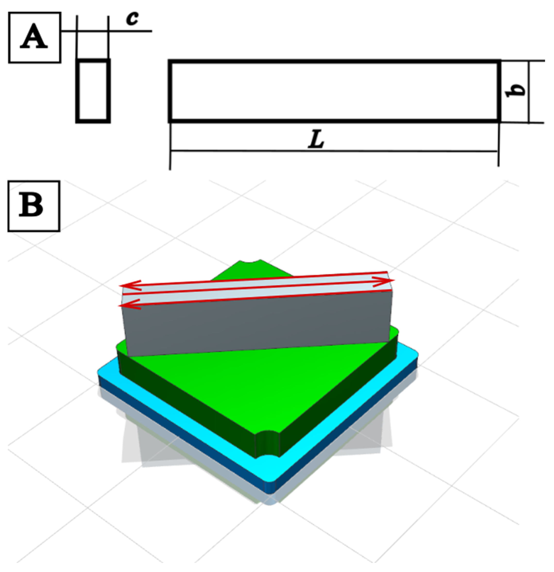
Figure 2. Schematic parameters of the SLM sample (A): L = 140 mm, b = 20 mm, and c ≈ 0.6 mm. The sample’s positioning on the table for printing (B). The scanning approach is conceptually represented by red arrows.
Jmmp 08 00235 g002
Figure 3. Samples were manufactured by SLM.
Jmmp 08 00235 g003
Figure 4. Dependence of the empirical probability density function (Equation (1)) on stress for SLM samples. (A)-without heat treatment; (B)-after heat treatment at 260 °C; (C)-after heat treatment at 290 °C; (D)-after heat treatment at 320 °C; (E)-after heat treatment at 350 °C; (F)-after heat treatment at 380 °C; (G)-after heat treatment at 410 °C; (H)-after heat treatment at 440 °C.
Jmmp 08 00235 g004
Figure 5. Dependence of the argument of the spectral density function as a function of stresses for SLM samples. (A)—without heat treatment; (B)—heat treatment at 260 °C; (C)—heat treatment at 290 °C; (D)—heat treatment at 320 °C; (E)—heat treatment at 350 °C; (F)—heat treatment at 380 °C; (G)—heat treatment at 410 °C; (H)—heat treatment at 440 °C.
Jmmp 08 00235 g005
Figure 6. Dependence of σT (transition stress) on annealing temperature (A) on strain hardening coefficient (θ) from yield strength to tensile strength (B).
Jmmp 08 00235 g006
Figure 7. Fracture probability density of bound states (14) for SLM samples. (A)—without heat treatment; (B)—after heat treatment at 260 °C; (C)—after heat treatment at 290 °C; (D)—after heat treatment at 320 °C; (E)—after heat treatment at 350 °C; (F)—after heat treatment at 380 °C; (G)—after heat treatment at 410 °C; (H)—after heat treatment at 440 °C.
Jmmp 08 00235 g007
Figure 8. Comparison of empirical fracture probability density (1) with theoretical fracture probability density (15) of samples No. 1 (A) and No. 2 (B) fabricated by selective laser melting technology from AlSi10Mg and heat-treated at 440 °C.
Jmmp 08 00235 g008
Table 1. The average chemical composition of AlSi10Mg powder.
ElementsAlSiMgO
Composition (wt. %)88.18509.95500.32751.5325
Table 2. Estimation of the closest distribution type to the left and right of the transition point σT by the Akaike and Bayesian information criteria.
No of SamplesHeat Treatment Temperature, °CDistribution to the Left of σTDistribution to the Right of σTb by Weibull, to σTa by Weibull, to σTb by Weibull, from σTa by Weibull, from σT
120WeibullWeibull92.2611.906254.5755.944
2WeibullWeibull92.0511.890255.6876.027
3WeibullWeibull93.8391.937258.1705.924
4WeibullWeibull94.3711.898260.6105.984
5WeibullWeibull99.0711.963270.3915.999
6WeibullWeibull97.3061.911270.0895.898
1260WeibullWeibull104.0332.024277.5446.016
2WeibullWeibull103.1112.043276.0526.005
3Normal *Weibull90.06347.118276.5955.984
4Normal *Weibull90.04445.315269.8655.947
5Normal *Weibull89.98047.091276.2795.965
6WeibullWeibull105.5442.064281.8725.981
1290WeibullWeibull112.8422.604281.0125.944
2WeibullWeibull107.1852.128281.5076.025
3Normal *Weibull95.20248.901288.4876.049
4Normal *Weibull90.95447.085277.0215.998
5Normal *Weibull88.59344.323267.2455.977
6WeibullWeibull105.5442.064281.8725.981
1320WeibullWeibull94.7922.120250.4516.081
2Normal *Weibull79.53441.247241.8675.968
3Normal *Weibull81.49541.480246.8036.024
4Normal *Weibull82.48841.084248.4626.003
5Normal *Weibull81.52743.051252.8255.993
6Weibull Weibull95.5882.182249.3686.065
1350Normal *Weibull74.50339.728230.7895.976
2WeibullWeibull87.5622.004236.0176.054
3Normal *Weibull78.11742.308247.1355.906
4Normal *Weibull75.43939.915235.3295.911
5Normal *Weibull76.27841.969243.5205.901
6WeibullWeibull86.5051.907239.6405.934
1380WeibullWeibull71.4801.987196.7895.975
2Normal *Weibull63.22233.497198.7815.940
3WeibullWeibull73.1442.108197.1605.988
4Normal *Weibull63.03832.635196.2545.943
5Normal *Weibull64.70433.599201.0266.009
6Normal *Weibull63.73833.586199.6725.962
1410Normal *Weibull51.43025.870158.8546.148
2WeibullWeibull62.1502.066170.4626.092
3Normal *Weibull54.69726.289159.9836.096
4Normal *Weibull49.75525.972157.1286.027
5Normal *Weibull51.01026.393163.0116.079
6Normal *Weibull51.87925.945162.5736.043
1440Normal *Weibull45.48222.385139.7556.158
2WeibullWeibull52.5732.283139.4836.218
3WeibullWeibull53.6852.204146.3326.230
4Normal *Weibull47.31023.696147.3956.139
5Normal *Weibull48.06623.824148.9536.226
6Normal *Weibull45.95622.924142.5936.141
* For the normal (6) distribution, the values of the mathematical expectation and mean square deviation of the stresses of the theoretical distribution established by the Akaike and Bayes criteria are given.
Table 3. Values of correlation coefficients and calculated level of statistical significance between the parameters of the distributions (Table 2) and the main mechanical properties [25].
Correlating PairsSpearman’s Correlation CoefficientEstimated Value of Statistical Significance Level
b_left—σ0.20.8652.343 × 10−15
b_left—σU0.933<2.2 × 10⁻¹⁶
b_left—ε0.20.8417.314 × 10−14
b_left—εU−0.6271.822 × 10−06
a_left—σ0.20.1930.189
a_left—σU0.0020.991
a_left—ε0.2−0.0950.520
a_left—εU−0.3330.021
b_right—σ0.20.934<2.2 × 10⁻¹⁶
b_right—σU0.989<2.2 × 10⁻¹⁶
b_right—ε0.20.8596.015 × 10−15
b_right—εU−0.7032.59 × 10−8
a_right—σ0.2−0.4370.002
a_right—σU−0.4670.001
a_right—ε0.2−0.4790.001
a_right—εU0.4400.002
Table 4. Robust regression equations linking the main mechanical properties and distribution coefficients.
EquationSDNo Eq.
b l e f t = 15.06 + 0.03 × σ 0.2 + 0.27 × σ B + 12.08 × ε 0.2 + 1.25 × ε B 5.657(19)
a l e f t = 35.0176 3.3086 × ε B 27.220(20)
b r i g h t = 0.70 + 0.18 × σ 0.2 + 0.71 × σ B 4.52 × ε 0.2 + 1.28 × ε B 1.485(21)
a r i g h t = 5.977 + 0.003 × σ 0.2 0.002 × σ B 0.096 × ε 0.2 + 0.049 × ε B 0.056(22)
Table 5. Deviations (16) in the theoretical fracture probability density (15) from the empirical one (1) for the samples made by selective laser melting technology from AlSi10Mg.
No of SamplesHeat Treatment Temperature, °CDeviation of Theory from Empirics (15), %
1203.986 × 10−3
23.925 × 10⁻³
33.840 × 10⁻³
43.745 × 10⁻³
53.414 × 10⁻³
63.408 × 10⁻³
12604.007 × 10−3
24.072 × 10⁻³
33.940 × 10⁻³
44.019 × 10⁻³
53.710 × 10⁻³
63.725 × 10⁻³
12904.163 × 10−3
23.876 × 10⁻³
33.579 × 10⁻³
44.039 × 10⁻³
54.095 × 10⁻³
63.861 × 10⁻³
13204.351 × 10−3
24.735 × 10⁻³
34.458 × 10⁻³
44.371 × 10⁻³
54.086 × 10⁻³
64.388 × 10⁻³
13504.398 × 10−3
24.197 × 10⁻³
33.655 × 10⁻³
44.164 × 10⁻³
53.776 × 10⁻³
63.974 × 10⁻³
13805.635 × 10−3
25.422 × 10⁻³
35.657 × 10⁻³
45.668 × 10⁻³
55.272 × 10⁻³
65.367 × 10⁻³
14107.045 × 10−3
26.551 × 10⁻³
36.899 × 10⁻³
46.952 × 10⁻³
56.784 × 10⁻³
66.917 × 10⁻³
14407.962 × 10−3
28.117 × 10⁻³
37.009 × 10⁻³
46.927 × 10⁻³
56.755 × 10⁻³
67.467 × 10⁻³
Disclaimer/Publisher’s Note: The statements, opinions and data contained in all publications are solely those of the individual author(s) and contributor(s) and not of MDPI and/or the editor(s). MDPI and/or the editor(s) disclaim responsibility for any injury to people or property resulting from any ideas, methods, instructions or products referred to in the content.