Next Article in Journal
Mission-Oriented Propulsion System Configuration and Whole Aircraft Redundancy Safety Performance for Distributed Electric Propulsion UAVs
Previous Article in Journal
Application of LMM-Derived Prompt-Based AIGC in Low-Altitude Drone-Based Concrete Crack Monitoring
 
 
Correction published on 15 October 2025, see Drones 2025, 9(10), 713.
Article

UAV Path Planning in Threat Environment: A*-APF Algorithm for Spatio-Temporal Grid Optimization

1
Equipment Management and Unmanned Aerial Vehicle Engineering School, Air Force Engineering University, Xi’an 710051, China
2
National Key Laboratory of Unmanned Aerial Vehicle Technology, Xi’an 710051, China
3
The Youth Innovation Team of Shaanxi University, Xi’an 710051, China
*
Author to whom correspondence should be addressed.
Drones 2025, 9(9), 661; https://doi.org/10.3390/drones9090661
Submission received: 25 July 2025 / Revised: 15 September 2025 / Accepted: 16 September 2025 / Published: 22 September 2025 / Corrected: 15 October 2025

Abstract

Highlights

What are the main findings?
  • A new global subdivided spatio-temporal grid system is proposed, which integrates the advantages of GeoSOT binary coding and BeiDou grid location code subdivision rules.
  • Based on the above-mentioned spatio-temporal grid system, threat quantification models for ground units such as radars, artillery, and interference are constructed. The traditional A* algorithm and artificial potential field (APF) algorithm are improved to enable each to adapt to the constructed complex threat environment. Experimental results show that the proposed A* algorithm is superior to the traditional algorithm in terms of path length, calculation time, threat value, and number of search nodes; the improved APF algorithm achieves 100% safe obstacle avoidance in dynamic obstacle environments.
What is the implication of the main finding?
  • The designed global subdivided spatio-temporal grid system has become a new way of spatio-temporal data storage, which can provide new ideas for the management and application of UAV swarms in complex threat environments.
  • The proposed A*-APF algorithm effectively solves the challenges of low threat avoidance efficiency and poor global path adaptability in UAV path planning in threat environments, and provides a new solution for UAV path planning in complex scenarios.

Abstract

To address low threat avoidance efficiency and poor global path adaptability in UAV path planning under threatening environments, this paper proposes a hybrid A*-Artificial Potential Field (APF) path planning method based on spatio-temporal grid optimization. First, a new global fine-grained spatio-temporal grid system is developed by integrating advantages of GeoSOT binary encoding and BeiDou grid location code subdivision rules, enabling unified modeling of complex spatio-temporal environments. Ground threat and maze scenarios are constructed for verification. Second, traditional A* and APF algorithms are improved: the A* algorithm is enhanced with threat costs, dynamic neighborhood search, and local backtrack mechanisms to address low efficiency and incompatibility with threat avoidance; the APF algorithm is optimized with a dual gravitational field collaboration mechanism and distance-parameter-based repulsive field model to overcome local minima and unreachable goals. Finally, a sliding window-driven path association model achieves seamless collaboration between global and local planning. Experimental results show the proposed method outperforms traditional algorithms in comprehensive performance, with the improved A* algorithm excelling in path length, computation time, threat value, and search nodes, and the improved APF algorithm achieving complete safe obstacle avoidance in dynamic environments. The collaborative mechanism effectively handles complex scenarios.

1. Introduction

The application of unmanned aerial vehicles (UAVs) in high-risk environments such as nuclear facility operations, deep space exploration, and battlefield reconnaissance is increasingly widespread. Efficient path planning is one of the key challenges in these applications [1]. UAV path planning is a crucial aspect of the autonomous control module, with the main task of designing an optimal flight path from the starting point to the destination while meeting the UAV performance requirements and minimizing costs [2].
There are mainly three types of existing environmental frameworks for path planning: local single-scale grid system [3], latitude–longitude system [4], and global subdivided grid system [5,6]. The first two belong to traditional frameworks. Among them, the local single-scale grid system is relatively simple to model, but the coordinate system needs to be rebuilt every time the path planning algorithm is applied in real-world scenarios, which is resource-intensive. The latitude–longitude system is essentially a vector description that can depict obstacle contours when fully sampled, but it is difficult to characterize regional geographical features, and the complexity of vector calculations can easily lead to efficiency bottlenecks. In summary, both the local single-scale grid system and the latitude–longitude system have efficiency limitations when used as environmental organizational frameworks for path planning problems. In contrast, the global subdivided grid system, by constructing multi-scale adjustable grids and unifying raster and vector data under spatio-temporal attributes, provides a more optimal data organization method for environmental discretization. However, existing global subdivided grid systems such as Geosot [7] (Geographic coordinate subdividing grid with one-dimension integral coding on 2n-tree) and BeiDou grid location code [8] also have certain limitations. Specifically, Geosot achieves binary encoding through virtual expansion (e.g., expanding both latitude and longitude ranges to (−256°–256°), with 1° expanded to 64′, and 1′ expanded to 64″), but this results in storage redundancy and issues with grid blockiness, readability, and identifiability in practical applications.The BeiDou grid location code abandons the virtual expansion method, but its mixed encoding of letters and decimal numbers is not conducive to binary storage in computers. Therefore, there is an urgent need to integrate the advantages of Geosot binary encoding with the BeiDou grid subdivision rules to construct a new global subdivision grid system.
In complex environments, UAVs need to perform global path planning to find the optimal route, ensuring efficient and safe arrival at the destination. Meanwhile, to avoid sudden threats (such as radar, artillery, interference, obstacles, and other factors that affect the safety of UAVs), UAVs need to utilize local path planning to dynamically perceive surrounding information and adjust their attitudes, ensuring safe avoidance of threat areas during flight. Global static planning algorithms include Dijkstra algorithm [9], A* algorithm [10], RRT (Rapidly-exploring Random Tree) algorithm [11], and GA (Genetic Algorithme) [12], among others. Local dynamic planning algorithms include DWA (Dynamic Window Approach) [13], APF (Artificial Potential Field) [14], and others.
The A* algorithm combines the advantages of uniform cost search and greedy search, ensuring an optimal path. However, real battlefield environments are complex and intricate. The areas where UAVs perform path planning are not simply judged by binary divisions for passability (e.g., 0 for passable, 1 for impassable). Instead, they require balancing multiple conflicts between path distance, computation time, and threat intensity. Recently, some scholars have conducted research based on the traditional A* algorithm. In their approach, they do not solely focus on the shortest path or the simplest route but comprehensively consider various factors within the airspace. Although this path may be slightly longer or more complex, it minimizes threats or other safety risks to the greatest extent possible. For example, Yang et al. [15] introduced a dynamic congestion quantification model into the original cost function and designed an adaptive weight factor to improve the A* algorithm, significantly enhancing the robot’s travel efficiency with a slight sacrifice in path length. Wei et al. [6] improved the A* algorithm by comprehensively considering path length, traffic volume, and safety risks, thereby significantly enhancing its adaptability and safety in actual complex airspace. However, their research methods are difficult to adapt to the global subdivided grid system. Therefore, how to integrate threat costs in complex battlefield environments into the cost function [16,17] while ensuring its compatibility with the global subdivided grid system [5,6,18] is one of the key challenges in optimizing path planning to meet future combat needs, and it is also the problem that this paper aims to solve.
The APF algorithm is a simple and widely applied method, which not only boasts advantages such as straightforward mathematical description and ease of real-time control but also demonstrates strong portability, making it suitable for local dynamic obstacle avoidance problems. The traditional APF algorithm is prone to falling into local minima. Some scholars have made improvements to address this issue. For example, Li et al. [19] proposed an improved APF algorithm based on chaos theory; Chen et al. [20] combined angle functions and fuzzy control ideas with the traditional APF algorithm; Lu et al. [21] improved the APF by refining the target fitting curve and critical oscillation points, achieving a balance between safe obstacle avoidance and path smoothness for UAVs.
To sum up, in high-threat battlefield environments, the mission planning of UAV swarms faces two core challenges: First, at the environmental level, existing grid systems mostly focus on spatial dimension subdivision and lack the integrated modeling of temporal dynamics, making it difficult to meet the demand for real-time situational awareness in complex threat environments. Second, at the algorithm level, traditional path planning algorithms (such as A* and APF) have defects in balancing dynamic obstacle avoidance and threat quantification, manifested as low obstacle avoidance efficiency and poor global path adaptability. Although GeoSOT binary coding has the advantage of efficient spatial indexing and BeiDou grid location code subdivision rules provide a basis for regional adaptability, the two have not been effectively integrated, resulting in a technical gap characterized by spatio-temporal data fragmentation and insufficient algorithm adaptability. Therefore, constructing a new grid system integrating spatio-temporal characteristics and developing adaptive optimization algorithms has become a key breakthrough to improve the reliability of UAV swarms’ mission execution in high-threat environments. In view of this, this paper takes the “global subdivided spatio-temporal grid in complex threat environments” as the environmental framework and designs a “real-time triggered local dynamic replanning mechanism” aiming at the impact of sudden threats on global key nodes. The scheme integrates the improved A* algorithm, APF algorithm, and a multi-granularity grid trajectory association model driven by sliding windows to achieve complementary advantages and enhance the comprehensive planning performance in complex threat environments.
The core contributions of this study include three aspects: First, a global subdivided spatio-temporal grid system integrating GeoSOT binary coding and BeiDou grid location code subdivision rules is proposed, which realizes the integrated storage and indexing of spatio-temporal data in battlefield environments for the first time and provides a novel technical framework for complex scenario modeling. Second, a multi-dimensional threat quantification model is constructed, and improvements are made to address the defects of traditional A* algorithm and artificial potential field (APF) algorithm in threat environments. Experiments verify that the improved algorithms are significantly superior to traditional methods in terms of path length, computational efficiency, and threat avoidance rate. Third, a collaborative A*-APF path planning mechanism is established, which effectively resolves the core contradiction of “threat avoidance-efficiency preservation” through spatio-temporal grid optimization methods, providing a reference paradigm for the improvement of intelligent algorithms and environmental modeling research.
The structure of this paper is as follows: Section 2 introduces spatio-temporal grid modeling, threat/maze scenario modeling, and the design of the path planning scheme; Section 3 verifies the robustness of the model and its superiority over current traditional algorithms through experiments in threat/maze scenarios. An overview of the A*-APF path planning scheme with spatio-temporal grid optimization in a complete threat environment is shown in Figure 1.

2. Related Methods

2.1. Spatio-Temporal Grid Modeling

2.1.1. Spatial Grid Division

To address the processing requirements of multi-source data in complex environments, this paper proposes a spatial environment modeling method based on a global subdivision grid system, aiming to provide a unified structured representation and computational framework for airspace data in UAV missions.
Based on the fundamental theory of three-dimensional subdivided grids in geospatial, this method conducts grid modeling of the airspace environment for UAV. The benchmark for spatial grid subdivision is set as the Earth’s reference ellipsoid, and a three-dimensional orthogonal coordinate system is established with the intersection of the prime meridian and the equatorial plane as the origin. The grid coverage spans globally in the longitudinal direction (±180°) and the latitudinal direction (±90°), extending from −6302 km below the Earth’s surface to 528,680 km above it in the vertical direction, forming a multi-level grid system with seamless global coverage. The hierarchical division strictly follows the principles of equal longitude-latitude differences and equal altitude differences, constructing a continuous, seamless, and non-overlapping multi-level three-dimensional grid system through progressive subdivision, with the smallest-volume element reaching the centimeter scale.
In terms of latitude and longitude, the grid levels are divided according to spatial resolution: Levels 1–9 represent degree-level grids, Levels 10–13 represent minute-level grids, Levels 14–17 represent second-level grids, and Levels 18–25 represent below second-level grids.
In the vertical direction, the grid levels are divided by resolution: Levels 1–15 represent kilometer-scale grids, Levels 16–17 represent hundred-meter-scale grids, Levels 18–19 represent ten-meter-scale grids, Levels 20–21 represent meter-scale grids, and Levels 22–23 represent centimeter-scale grids. The minimum scale is at the ten-centimeter level, which meets the requirements of UAV mission planning. The actual subdivision effect is shown in Figure 2.
After completing spatial grid subdivision, it is necessary to assign unique encodings to grid cells to determine their spatial positions. This study adopts a binary encoding scheme to support airspace grid calculations.
  • Coding length and level identification. The coding length for each dimension is fixed at 32 binary digits. For a given level (N2 = 13), the effective number of bits is 16. Therefore, the latter 16 bits of the latitude coding (the level identification code element part) consist of 1 bit of “0” (indicating the end of the level) and 15 bits of “1” (padding bits). Similarly, the effective number of bits for the height level N3 = 16 is 18.
  • Encoding Latitude and Longitude. For latitude (34°24′58.379″ N), the first code element: the Northern Hemisphere (N) is identified as “0”; the degree value (34°) is converted to a 9-bit binary number “000100010” (with leading zeros to make 9 bits); the minute value (24′) is converted to a 7-bit binary number “0101100”; the second value (58″) is converted to a 7-bit binary number “1110011”; the fractional part of the second (0.379″) is converted to an 8-bit binary number “01100001”. Combining these parts and adding a 1-bit level identifier (the first “0” in the last 16 bits mentioned in Step 1), we obtain the complete 32-bit latitude code “0001000100101100111001101100001”. Based on an effective bit length of 16, the latitude code under N2 = 13 is “00010001001011000111111111111111”. Similarly, the longitude (109°3′41.260″ E) is encoded as “00110110100000110111111111111111111”.
  • Two-dimensional plane encoding. The obtained 32-bit latitude encoding and 32-bit longitude encoding are combined using Morton ordering to generate a unique 64-bit two-dimensional plane encoding. The result in this example is “0000011100010110010010001010010100111111111111111111111111111111”.
  • Height encoding. Based on an effective bit length of 18, the height encoding under N3 = 16 is “00000001000110000001111111111111”. See Figure 3 for a detailed diagram of the encoding process.

2.1.2. Temporal Grid Division

The battlefield threat environment possesses notable dynamic evolutionary characteristics, with the attributes and states of its constituent elements constantly changing over time. Relying solely on spatial dimension descriptions is insufficient for effectively organizing and managing battlefield spatio-temporal data. Therefore, based on the completion of spatial grid subdivision, it is necessary to introduce the temporal dimension and integrate its coding with spatial grid coding to construct an integrated spatio-temporal coding system.
To accommodate the diverse requirements of different combat missions and variations in UAV performance, this study first selects the spatial grid granularity based on a comprehensive consideration of spatial grid subdivision rules. Subsequently, the global time step (which also corresponds to the actual flight control period of the UAV) is dynamically adjusted using Equation (1):
Δ t l = 1 l · Δ t max
where Δ t max represents the global time step; l represents the number of levels for subdividing the global coarse-grained grid into fine-grained grids.
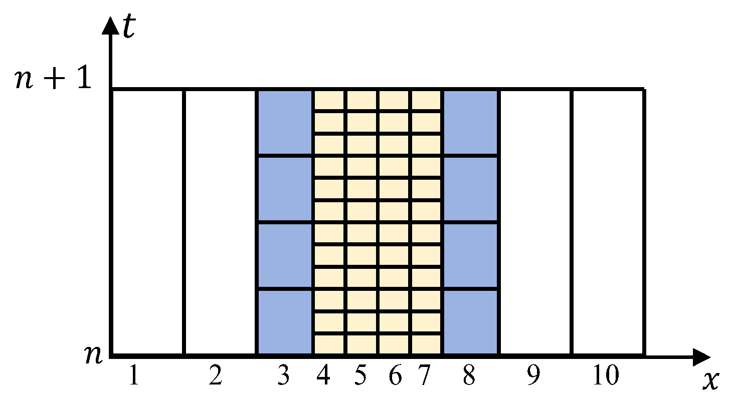
Regarding the explanation of Δ t l : As shown in Figure 4, grids 1, 2, 9, and 10 have a layer number l = 0 , grids 3 and 8 have a layer number l = 4 , and grids 4 to 8 have a layer number l = 12 . Initially, all grids are at time t n . The time step from t n to t n + 1 is Δ t max . Firstly, all grids are divided with a time step of Δ t max . Subsequently, grids 3 and 8 are calculated and updated with a time step of 1 4 Δ t max , at which point grids 3 and 8 are at time 1 4 Δ t max . Similarly, grids 4–7 are at time 1 12 Δ t max , and so on, until the smallest time step is obtained.

2.1.3. Multi-Granularity Spatio-Temporal Grid Division

In complex battlefield environments, airspace division is a key element in ensuring safe flight of unmanned aerial vehicles (UAVs) and efficiently avoid obstacle conflicts. When planning the flight track of UAV, the multi-grained grid design can significantly reduce the computational complexity of track planning: at a larger scale I, only the potential threats between coarse-grained sub-airspaces need to be considered; at a smaller scale II, the threats within the fine-grained sub-airspace are focused on. This strategy is more efficient and more scalable than evaluating all obstacles in the entire airspace in traditional methods. As shown on the left side of Figure 5, the UAV flight scenario includes multiple threat factors such as ground threat units, terrain, buildings, etc.; the right side of Figure 5 shows the structure of the scene divided into multi-scale, independent and non-overlapping multi-level grid sub-airspaces. Among them, coarse-grained path nodes are composed of N continuous sub-airspaces of scale I, which can be represented as [ CS 1 , CS 2 , , CS n , CS N ] ; fine-grained path nodes are composed of M continuous sub-airspaces of scale I, which can also be represented as [ FS 1 , FS 2 , , FS m , FS M ] . Specifically, the fine-grained path in Figure 5 can be expressed by four multi-grained nodes as [ CS 5 : FS 1 , CS 5 : FS 2 , CS 5 : FS 3 , CS 5 : FS 4 ] .

2.2. Complex Environment Modeling

2.2.1. Threat Scenarios Modeling

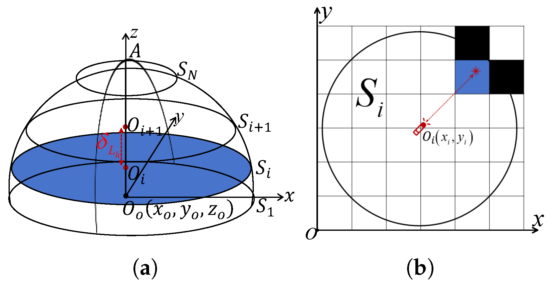
A hemisphere is used as a simplified geometric model of the ground threat unit’s scope. Suppose a threat unit has three-dimensional coordinates O o x o , y o , z o , with an area of effect radius of R. The edge length of the subdivided volume element at the L λ φ level in the longitude and latitude directions is δ λ φ , and the edge length of the subdivided volume element at the L h level in the height direction is δ h . The specific modeling process of the hemispherical model is as follows.
[Step1] Vertical subdivision: Subdivide the scope vertically into layers (Figure 6a), generating M clusters of equally spaced circular sections, where M is determined by R and δ h :
M = R δ h
R i = R 2 [ ( i 1 ) · δ h ] 2
[Step2] Horizontal filling: Employ the fast voxel traversal algorithm using ray tracing [22] to perform grid-based filling on M circular surfaces, constructing a horizontal subdivision structure (Figure 6b). Let the center coordinates of circle S i be O i x i , y i , and the filling rule is as follows:
( x , y ) | ( x x i ) 2 + ( y y i ) 2 N i 2
N i = R i δ λ φ
At time t, the distance between the UAV u and the ground threat unit s is D su ( t ) . The quantification method for the threat posed by enemy combat units is as follows.
(1) Radar unit
Assuming the maximum detection distance is R max , the scanning period is t r , and the beam swing angle is θ t . The threat quantification formula is
T r ( x , y , z , t ) = cos ( θ ( t ) ) 1 + D ij 4 / R max 4 , D su ( t ) R max 0 , D su ( t ) > R max
The dynamic model of the beam angle is as follows:
θ ( t ) = π 3 sin 2 π t t r
(2) Artillery unit
Assuming the maximum attack radius and high-risk attack radius of the artillery are R Amax and R Amin , respectively, the ammunition loading interval is t a , the duration of the firing window is δ t , and the time of the kth firing is t k . The threat value is zero during the loading period [ t k , t k + t a ] , and its threat quantification model is
T a ( x , y , z , t ) = 1 , D su ( t ) < R Amin R Amax D su ( t ) R Amax R Amin , R Amin D su ( t ) R Amax 0 , D su ( t ) > R Amax
During the loading time, the threat level always satisfies the following:
T a ( x , y , z , t ) = 0 , if t mod ( t a + Δ t ) t a
(3) Interference unit
Assuming the maximum effective interference radius and high-risk interference radius of the interference unit are R Imax and R Imin , respectively, the interference fluctuation period is t i , the interference power is P i ( t ) , and the interference power threshold constant is P t ( t ) . Its threat quantification model is
T i ( x , y , z , t ) = 1 , D su ( t ) < R Imin e 0.02 D su ( t ) R Imin , R Imin D su ( t ) R Imax 0 , otherwise
The dynamic model of interference power and effective radius is
P i ( t ) = 0.5· ( 1 + sin ( 2 π t t i ) )
R Imax = R Imin + P i ( t ) P t ( t )
Assuming the weight of the ground threat unit α i is η i and the threat value at point p is ω ( p , α i ) , the comprehensive threat value at that point is quantified as the formula:
T ( x , y , z , t ) = 1 i = 1 n η i ( 1 ω ( p , α i ) ) , p i = 1 n α i 0 , p i = 1 n α i

2.2.2. Maze Scenario Modeling

Randomly generate maze-like obstacle scenarios and input the obstacle information into spatial grids at various levels. Obstacle density ρ [ 0 , 1 ] , the larger ρ is, the denser the spatial distribution of obstacles is. To satisfy the dynamic range constraints, random fluctuations are introduced to the number of obstacles N obs according to Equation (14):
N obs = [ S 2 · ρ · 0.5 , S 2 · ρ · 1.5 ]
where S represents the grid size, and · represents the floor function. This constraint enhances the diversity of scene generation through a ±50% fluctuation while maintaining the global density characteristic ρ .
The correspondence between obstacles and grids is established through binary mapping as follows:
G r i d = { 0 , 1 } S
where 1 represents the obstacle-occupied grid, and 0 represents the accessible area.
In summary, the spatial classification criteria based on the threat index are as follows:
S p a c e T y p e ( p ) = Free - space , T ( p ) < 0.3 Competition - space , 0.3 T ( p ) 0.8 Denial - space , 0.8 < T ( p ) 1.0
In free space, both enemy and friendly UAVs can be used; in denied space, our UAVs are prohibited from being used; in competitive space, whether they can be used is determined by the combat unit, and if certain conditions are met, the three state spaces can be converted into each other.

2.3. Path Planning

UAV path planning mainly includes two key steps. Firstly, a continuous, coarse-grained path sequence, denoted as [ CS 1 , CS 2 , , CS n , CS N ] , is found in the static threat airspace based on the improved A* algorithm. If a sudden threat disturbance occurs in a certain subspace, a fine-grained path sequence, also denoted as [ FS 1 , FS 2 , , FS m , FS M ] , is generated along the guided path within the disturbed subspace based on the improved APF algorithm [23].

2.3.1. Path Planning Among Sub-Airspaces Based on Improved A* Algorithm

Dynamic Constraints of Unmanned Aerial Vehicles
Given that UAVs need to fly in complex airspace environments, clear constraints must be established based on their actual performance parameters. Assuming that after grid encoding, the current node coordinates are x i , y i , z i , and the adjacent node coordinates are also x i + 1 , y i + 1 , z i + 1 , then the direction vector of the unit path segment is defined as a i = x i + 1 x i , y i + 1 y i , z i + 1 z i .
(1) Minimum step size
The minimum step size refers to the minimum distance required for the UAV to maintain a straight-line flight state, which is usually related to the scale of the airspace grid.This parameter ensures that the UAV has enough space to complete attitude control during path adjustments, avoiding issues such as attitude oscillation, conflicting control commands, or increased collision risks due to excessively short step lengths. In this paper, it is stipulated that the minimum step length l min for UAVs must satisfy:
l min = min ( L o n i , L a t i , H e i g h t i )
where min ( L o n i , L a t i , H e i g h t i ) represents the grid side lengths δ λ φ and δ h in the latitude, longitude, and altitude directions at the current grid level.
(2) Maximum yaw angle
The maximum yaw angle refers to the maximum turning angle allowed for the UAV in the horizontal direction. By limiting the turning radius, it is possible to avoid excessive centrifugal force or accumulation of positioning errors caused by sharp turns. In this paper, a right turn is defined as the positive direction, and the maximum yaw angle Δ ψ max of the UAV must satisfy:
Δ ψ = arccos a i 1 T · a i a i 1 a i Δ ψ max
where, a i 1 and a i are the direction vectors of the (i-1)th and ith path segments in the flight path, respectively.
(3) Maximum pitch angle
The maximum pitch angle refers to the maximum climb or descent angle allowed for the UAV in the longitudinal plane. Due to the structural characteristics of UAVs, climbing or descending at excessive angles can easily induce a “stall” condition. In this paper, the upward movement of the nose is defined as the positive direction, and the maximum pitch angle Δ θ max of the UAV must satisfy the following:
Δ θ = arcsin z i z i 1 a i 1 Δ θ max
where z i 1 and z i represent the height coordinates of the starting point and ending point of the ith path segment, respectively.
(4) Roll angle
Given the presence of numerous obstacles in complex airspace environments, the rolling motion of UAVs can significantly alter their safety buffer zones, greatly increase computational complexity, and pose a high risk of collision. Therefore, this paper strives to avoid the use of rolling maneuvers in path planning research.
Optimizing Cost Function Design
Define the three-dimensional discrete grid state space as G = ( x , y , z ) Z 3 , where the space boundaries satisfy x 0 , X max , y 0 , Y max , z 0 , Z max . The current node (includes both coordinates and attributes) attributes are represented as n i = ( x i , y i , z i ) , T i , φ i , θ i , f i , where ( x i , y i , z i ) are the node’s three-dimensional coordinates, T ( p ) 0 , 1 represents the threat value, φ i φ max , φ max represents the yaw angle information, θ i θ max , θ max represents the pitch angle information, and f i represents the cost value information. The starting node is denoted as C S s = ( x s , y s , z s ) G , the goal node as C S g = ( x g , y g , z g ) G , and the historical path node sequence as P = C S s , C S 2 , , C S i , , C S g .
Based on the above definitions and characteristics of the airspace grid environment, the optimized cost function is
f ( C S i ) = α g g ( C S i ) + α h h ( C S i ) + α c · c ( C S i )
where g ( C S i ) represents the cumulative path cost function; h ( C S i ) represents the heuristic function; c ( C S i ) represents the motion threat penalty function; α g , α h , α c are the weighting factors, satisfying α g + α h + α c = 1 and α g , α h , α c > 0 .
(1) Accumulated Path Cost g ( C S i )
It represents the accumulated cost of the actual path from the starting node C S s to the current node C S i . The calculation is based on the Euclidean distance as the fundamental distance cost metric, aligning with the movement characteristics of UAVs in a three-dimensional grid space. To ensure path smoothness, under hard constraints such as yaw angle and pitch angle, soft constraint costs for yaw angle and pitch angle are introduced [24]. The cumulative path cost function is designed as follows:
g ( C S i ) = k = 1 i β l · Δ p k + β ψ · Δ ψ k + β θ · | Δ θ k |
where β l , β ψ and β θ are the weight coefficients for distance, yaw, and pitch, respectively, satisfying β l + β ψ + β θ = 1 and β l , β ψ , β θ > 0 ; the expressions for Δ p k , Δ ψ k and Δ θ k are
Δ p k = ( x k x k 1 ) 2 + ( y k y k 1 ) 2 + ( z k z k 1 ) 2 Δ ψ k = arccos a k 1 · a k a k 1 a k Δ ψ max Δ θ k = arcsin | z k z k 1 | a k 1 Δ θ max
(2) Heuristic Function h ( C S i )
The heuristic function represents the minimum expected cost from the current node C S i to the target node C S g , guiding the search direction. It employs a three-dimensional Chebyshev distance metric and introduces a threat weighting term to enhance path guidance:
h ( C S i ) = max | x i x g | , | y i y g | , | z i z g | · B A + w ¯ k
where:
  • A and B represent the horizontal and vertical grid scales, respectively.
  • The z-axis difference is scaled to match horizontal dimensions using B A .
  • w ¯ k is the average threat value of detected nodes, estimating threat in unexplored areas.
(3) Threat Cost Function c ( C S i )
The threat cost function defines threat information based on a three-dimensional grid as follows:
c ( C S i ) = T ( p )
Dynamic Neighborhood Search
As shown in Figure 7, the UAV motion model includes modes such as two-dimensional four-neighborhood Figure 7a, eight-neighborhood Figure 7b, three-dimensional six-neighborhood Figure 7c, and twenty-six-neighborhood Figure 7d [25]. Considering the actual flight operation of UAV, this study adopts the twenty-six neighborhood motion rule. When the UAV is disturbed by environmental threats, it may deviate from the target direction, leading to local oscillation phenomena and significantly increasing path length, flight duration, and energy consumption.
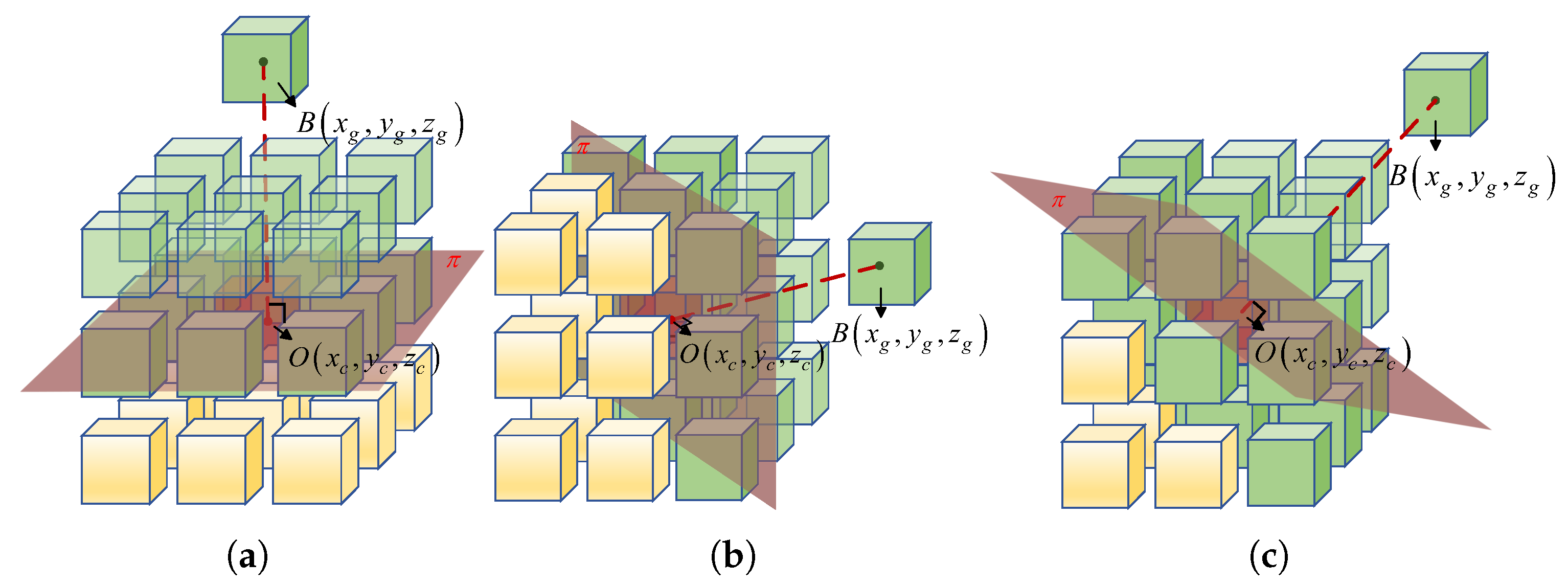
To enhance search efficiency, a dynamic neighborhood search strategy is proposed: adaptively adjusting the neighborhood size by predicting the flight direction. As shown in Figure 8, assuming the current node is O ( x c , y c , z c ) , the target node is B ( x g , y g , z g ) , and the candidate neighborhood node is P ( x n , y n , z n ) . A plane π passing through point O and perpendicular to the vector O B is constructed. Based on pre-similarity screening, neighborhood nodes on the target direction side (angle 90 ) are selected using the following condition:
S = v g · v n || v g || || v n || 0 v g = ( x g x c , y g y c , z g z c ) v n = ( x n x c , y n y c , z n z c )
Figure 8a shows the case where plane π is parallel to the coordinate axes, with the number of neighboring domains equal to 9; Figure 8b depicts the case where plane π is parallel to the face diagonals, also with the number of neighboring domains equal to 9; Figure 8c illustrates the case where plane π is parallel to the body diagonal, with the number of neighboring domains equal to 19. In general cases, the number of neighboring domains dynamically changes between 9 and 19 based on the orientation of plane π .
Design of Local Backtracking Mechanism
In complex environments with wide threat ranges or dense obstacles, UAV path planning is prone to falling into local dead zones, leading to algorithm deadlock. To address this, this paper proposes a local backtracking path planning method: when the UAV is trapped in a dead zone, it expands its detection field to obtain more comprehensive environmental information and achieve path escape.
(1) Definition of Dead Zone
The criteria for determining a dead zone are as follows: in a competitive environment T ( p ) [ 0.3, 0.8] , if the proportion of grids with threat value exceeding 0.7 within the UAV’s 26-neighborhood exceeds threshold τ (typically τ = 0.8 ), it is considered a dead zone. The dead zone probability P dead is:
P dead = C S i N 26 ( C S i ) I T ( p ) > 0.7 | N 26 |
where I ( · ) is the indicator function, returning 1 if true, 0 otherwise.
(2) UAV Field of View Model
As shown in Figure 9, a zoom camera-like field of view model is introduced, defining the UAV’s detection range as a cuboid region centered at current position C S i = ( x i , y i , z i ) :
H ( C S i , k 1 , k 2 ) = ( x , y , z ) | x x i | k 1 | y y i | k 1 | z z i | k 2
where k 1 and k 2 are are the extension coefficients in the horizontal and vertical directions, respectively.
Set the dead-end node as C S i local = ( x i local , y i local , z i local ) , and perform local backtracking starting from this node with the modified cost function:
f ( C S i local ) = α g g ( C S i local ) + α h h ( C S i local ) + α c · c ( C S i local ) g ( C S i local ) = k = 1 i β l local · Δ p k local + β ψ local · Δ ψ k local + β θ local · | Δ θ k local | h ( C S i local ) = ω ¯ k local × max | x i x g | , | y i y g | , | z i z g | · B A c ( C S i local ) = T ( p )
where:
  • ω ¯ k local represents the inverse of the average threat value within the UAV’s field of view.
  • Local weights β l local , β ψ local , β θ local prioritize escape direction over path smoothness.
During the local backtracking phase, nodes are allowed to jump to the edge of the visible area. After finding the optimal boundary node, the A* algorithm described in Section 2.2.2 is invoked to generate a transitional path from the dead-end node C S i local = ( x i local , y i local , z i local ) to the optimal boundary node, and then reconnect it to the global plan.

2.3.2. Design of Trajector Association Model Driven by Sliding Window

Sliding Window Design
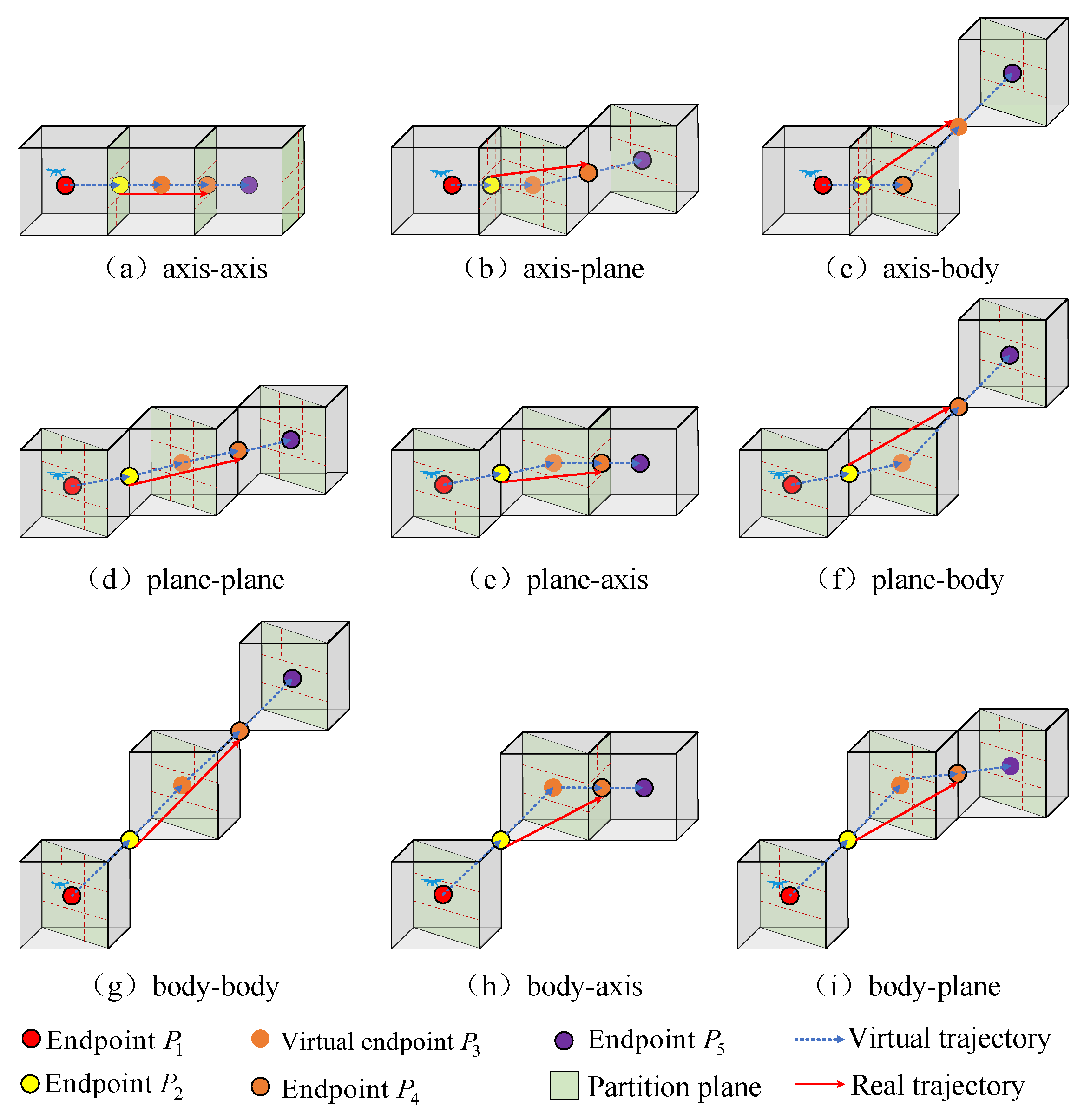
To reduce the risk of collisions, enhance path guidance among sub-airspaces, and improve planning efficiency, a multi-granularity path association model driven by a sliding window is designed [23]. As shown in Figure 10, the transitional trajectories between neighboring sub-airspaces encompass three categories with nine basic transformations: coordinate axis-aligned directions (abbreviated as “axis”), face diagonal directions (abbreviated as “face”), and space diagonal directions (abbreviated as “space”). Among them, solid dots with solid lines represent actual path nodes (such as P 1 , P 2 , P 4 , P 5 ), solid dots without solid lines represent virtual path nodes (such as P 3 ), blue dashed lines represent virtual guiding trajectories ( P 1 P 2 P 3 P 5 ), and red solid lines represent actual guiding trajectories ( P 1 P 2 P 4 P 5 ). The actual path is dominated by the attraction of grid entry and exit points, and smooth transitions in the path are achieved through dynamic associations between virtual and actual nodes.
The dynamic execution mechanism with a sliding window for path planning among sub-airspaces is shown in Figure 11a. The workflow is as follows: When the UAV enters the starting subspace C S 1 , the system initializes the sliding window and selects the set of sub-airspaces { C S 1 , C S 2 , C S 3 } within the blue dashed boundary as the sliding window (Sliding Window1). As the UAV moves from C S 1 to C S 2 , the window maintains the active status of { C S 2 , C S 3 } , generating feasible paths in real time. When the UAV fully enters C S 2 , the window dynamically updates to a new set of sub-airspaces within the red solid boundary (Sliding Window2), and the process of window sliding and updating is repeated. The window sliding terminates when the number of remaining sub-airspaces to be planned is less than three.
The key elements in Figure 11a are as follows:
  • Actual path nodes: { P 1 , P 3 , P 4 , P 6 , P 8 , P 9 } .
  • Virtual path guidance nodes: { P 2 , P 5 , P 7 } .
Path Guidance Strategy
The path generated based on the sliding window is shown in Figure 11b, and its guidance mechanism is defined as follows: Suppose A ( x s , y s , z s ) is the starting point of the guidance path within the subspace, B ( x g , y g , z g ) is the endpoint, and C ( x c , y c , z c ) is the real-time position of the UAV. Define D ( x d , y d , z d ) as the foot of the perpendicular from point C to the line AB. With AB as the ideal guidance path, an evaluation index for path adherence is established.
Path deviation: The Euclidean distance from the UAV to the guidance path is defined as follows:
d = C D
Course deviation angle: The angle between the current course B C and the guided route A B is defined as follows:
θ n = arccos B C · A B B C A B
Since the straight path AB is the theoretically optimal path within the subspace, the goal of path guidance is to achieve high adherence to the flight path by minimizing the deviation between d and θ n through real-time control.

2.3.3. Path Planning in Sub-Airspace Based on an Improved APF Algorithm

Addressing the contradiction between local dynamic obstacle avoidance and global optimality in traditional path planning algorithms, this paper proposes a hybrid A*-APF optimization algorithm. The algorithm employs a dual-mode layered architecture: an improved A* algorithm is used to generate discrete path sequence nodes among sub-airspaces. When sudden threats interfere with global path nodes, the system immediately switches to the local response layer to execute real-time obstacle avoidance within the subspace based on the APF method. A sliding window mechanism is utilized to dynamically guide the unmanned aerial vehicle (UAV) to avoid threats and automatically return to the global A* planned path after escaping the threat, achieving synergy between global optimization and local obstacle avoidance.
Improved Gravitational Potential Field
To address the local minimum problem of the traditional artificial potential field method, a dual gravitational field cooperation mechanism is proposed.
The goal gravitational field ( F att 1 ) within the subspace enhances the local target attraction:
F att 1 = k att 1 · 1 e q g q · q g q q g q
where k a t t 1 represents the gravitational gain coefficient; q g represents the final position; q represents the current position; 1 e q g q represents the distance attenuation factor, addressing the issue of unreachable targets.
Guide the gravitational field of the path( F att 2 ) to improve the path fit. Firstly, calculate the foot of the perpendicular A from the current position to the guidance path based on Equations (32) and (33). Secondly, construct the guidance path attraction force as shown in Equation (34).
t = max 0 , min 1 , q q s · q g q s q g q s 2
q D = q s + t · q g q s
F att 2 = k att 2 · e k · q D q · q D q q D q
where k att 2 represents the gravitational gain coefficient of the guidance path within the subdomain; k > 0 controls the intensity attenuation of gravity, which automatically reduces the gravitational force as the UAV approaches the guidance line to avoid path oscillation.
The total gravitational force acting on the UAV is the vector synthesis of the dual gravitational fields:
F att = F att 1 + F att 2
Improved Repulsive Potential Field
To address the issue of target unreachability, an improved repulsive potential field model based on distance parameters is proposed. Assuming the obstacle positions are q obs , the Euclidean distance is d obs = q q obs , and the minimum safe distance is d min . The improved piecewise expression for the repulsive force F rep is
F rep = k rep · 1 d min 1 ρ 0 · 1 d min λ · q q obs q q obs , d obs < d min k rep · 1 d obs 1 ρ 0 · 1 d obs λ · q q obs q q obs , d min d obs < ρ 0 0 , d obs > ρ 0
where k rep is the repulsive force gain coefficient; ρ 0 is the repulsive force influence radius; λ is the repulsive force attenuation exponent.
The resultant force acting on the UAV is the vector sum of the attractive and repulsive forces:
F total = F att 1 + F att 2 + F rep
UAV Motion Model in Sub-Airspace
(1) Adaptive step size
δ = 0.3· δ 0 , F total > 5 0.6· δ 0 , 2 < F total 5 δ 0 , 0.5< F total 2 1.5· δ 0 , F total 0.5
where δ 0 is the basic step size.
(2) Smooth processing of speed
v new = ( 1 η ) · F total F total + η · v old v new = v new v new
where η represents the inertia factor; v old represents the velocity before smoothing.
(3) Position update
q new = q old + δ · v new
(4) Path smoothing based on Savitzky–Golay filter
To address the issue of high-frequency oscillation caused by dynamic obstacle avoidance, Savitzky–Golay filtering is applied for post-processing. The filter is individually applied to each coordinate component of the original path sequence C F i = ( x i , y i , z i ) i = 1 n . An n-th order polynomial fit is used within the window m , m :
x t = k = 0 n a k t k
Optimize coefficients through least squares method:
min a k i = m m x i x t i 2
Its matrix solution is
a = A T A 1 A T x
where the elements of matrix A is A i j = t i j 1 ( i m , m + 1 , , m , j 1 , 2 , , n + 1 )
The smoothed value of the output window center point is x ^ 0 :
x ^ 0 = x ( 0 ) = a 0 = e 1 T a e 1 = [ 1 , 0 , , 0 ] T

3. Simulation Analysis

3.1. Environmental Settings

A three-dimensional battlefield environment is constructed based on grid generation rules: the spatial height is 3000 m and the longitude and latitude span is 0.042°. The global grid level is set to the 16th level for longitude/latitude (scale of 150 m) and the 17th level for height (scale of 100 m). Specific parameters are shown in Table 1.
During the path planning process, the starting and ending points within the subspace are dynamically selected based on sudden threats. A refined grid is adopted within the subspace: the 19th level for longitude/latitude (with a scale of 7.5 m) and the 20th level for altitude (with a scale of 5 m), constructing a three-dimensional grid environment within the subspace.
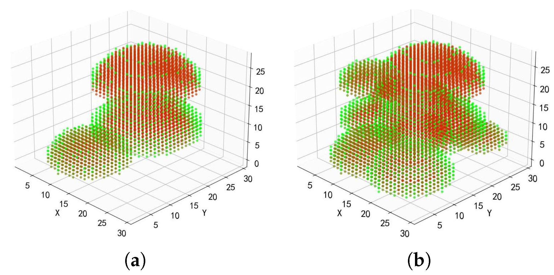
To verify the robustness of the algorithm, two typical threat scenarios are designed: a ground threat scenario (Figure 12) and a maze scenario (Figure 13).
(1) Ground threat scenario
Figure 12a represents a low-threat scenario with few threat types and low density; while Figure 12b represents a high threat scenario, with many types of threats and high density.
(2) Maze scenario
Under low-density conditions, the maze scenarios are shown in Figure 13a,b, while under high-density conditions, the maze-like threatening environments are depicted in Figure 13c,d.

3.2. Plan Planning Among Sub-Airspaces

To verify the performance of the improved A* algorithm proposed in this paper, two typical threat environments are set up for simulation experiments. In the experiments, the improved A* algorithm, traditional A* algorithm, Genetic Algorithm (GA), Simulated Annealing Algorithm (SA), and Q-learning algorithm will be compared and analyzed in terms of key performance indicators such as path length, algorithm time, total path threat value, and number of search nodes, in order to evaluate their superiority and advancement.

3.2.1. Ground Threat Scenario

In this scenario, the threat value distribution in the simulation environment is represented by a color gradient: the threat value gradually changes from green (low) to red (high). The path nodes obtained by different algorithms are marked in blue.
Simulation experiments are conducted for low, medium, and high levels of combat threat environments, respectively. The planning results are shown in Figure 14, Figure 15 and Figure 16. Specifically, Figure 14 displays the path planning results of various algorithms in a low-level threat scenario (few threat types, low density); Figure 15 shows the results in a medium-level threat scenario; and Figure 16 presents the results in a high-level threat scenario (many types of threats and high density).
Table 2 summarizes the detailed performance comparison data of five algorithms in terms of path length, algorithm time, total path threat value, and the number of search nodes under the aforementioned combat threat environments.

3.2.2. Maze Scenario

To evaluate the performance of algorithms in complex obstacle environments, simulation experiments were conducted in a maze environment. In the experiments, the performance of the improved A* algorithm, traditional A* algorithm, GA, SA, and Q-learning algorithm in path planning was compared and analyzed. The planning results are shown in the following figures. Figure 17, Figure 18 and Figure 19. respectively show the planning results of different algorithms in the scenarios of ρ = 0.2 , ρ = 0.5 , and ρ = 0.8 . Table 3 summarizes the detailed performance comparison data of the above five algorithms in terms of path length, algorithm time, total path threat value, and the number of search nodes in the maze environment.

3.2.3. Result Analysis

As shown in Table 2, the improved A* algorithm demonstrates significant performance enhancements in combat environments with low, medium, and high threat levels. The detailed analysis is shown in Table 4 and Table 5.
Comparison with the Traditional A* Algorithm
(1) Low-threat scenario
The path length is shortened by 10.90%, the computation time is reduced by 73.34%, the total path threat value is decreased by 25.04%, and the number of search nodes is reduced by 64.29%.
(2) Medium-threat scenario
The path length is shortened by 13.46%, the computation time is reduced by 61.99%, the total path threat value is decreased by 8.24%, and the number of search nodes is reduced by 65.52%.
(3) High-threat scenario
The path length is shortened by 8.34%, the computation time is reduced by 79.35%, the total path threat value is decreased by 56.60%, and the number of search nodes is reduced by 61.54%.
Comparison with Other Intelligent Algorithms
(1) Low-threat scenario
  • Path Length: Reduced by 18.18%, 11.79%, and 26.10% compared to GA, SA, and Q-learning, respectively;
  • Computation Time: Decreased by 17.01%, 22.47%, and 83.95% compared to GA, SA, and Q-learning, respectively;
  • Total Path Threat Value: Lowered by 50.21%, 50.37%, and 3.01% compared to GA, SA, and Q-learning, respectively.
(2) Medium-threat scenario
  • Path Length: Shortened by 21.00%, 15.31%, and 30.04% compared to GA, SA, and Q-learning, respectively;
  • Computation Time: Reduced by 12.39%, 16.42%, and 75.71% compared to GA, SA, and Q-learning, respectively;
  • Total Path Threat Value: Decreased by 42.86%, 53.75%, and 9.25% compared to GA, SA, and Q-learning, respectively.
(3) High-threat scenario
  • Path Length: Cut by 19.80%, 11.04%, and 30.69% compared to GA, SA, and Q-learning, respectively;
  • Computation Time: Decreased by 11.67%, 20.20%, and 74.35% compared to GA, SA, and Q-learning, respectively;
  • Total Path Threat Value: Reduced by 49.03%, 54.67%, and 43.00% compared to GA, SA, and Q-learning, respectively.
(Note: Table 3 presents relevant data using the same analysis method and will not be elaborated here.)
Compared with the traditional A* algorithm, the improved A* algorithm reduces the average path length by 10.9%, the calculation time by 71.56%, the cumulative threat value by 29.96%, and the number of search nodes by 63.78%; compared with other traditional intelligent algorithms, the path length is shortened by an average of 20.44%, the calculation time is reduced by 37.13%, and the cumulative threat value is reduced by 32.24%.
In terms of computational complexity, the proposed improved A* algorithm reduces the number of nodes expanded in each search by approximately 26.9–65.4% through the dynamic neighborhood search strategy (retaining only 9–19 neighbor nodes on the target direction side instead of the traditional 26 neighborhoods), significantly reducing the computational overhead caused by invalid searches. Combined with the adaptive field-of-view model in the local backtracking mechanism (dynamically adjusting the detection range via expansion coefficients k 1 and k 2 ), redundant computations from global traversal are avoided. As a result, the computation time in high-threat scenarios is reduced by 79.35% compared to the traditional A* algorithm and by 20.20% compared to the SA algorithm (see Table 4 and Table 5).

3.3. Path Planning in Sub-Airspace

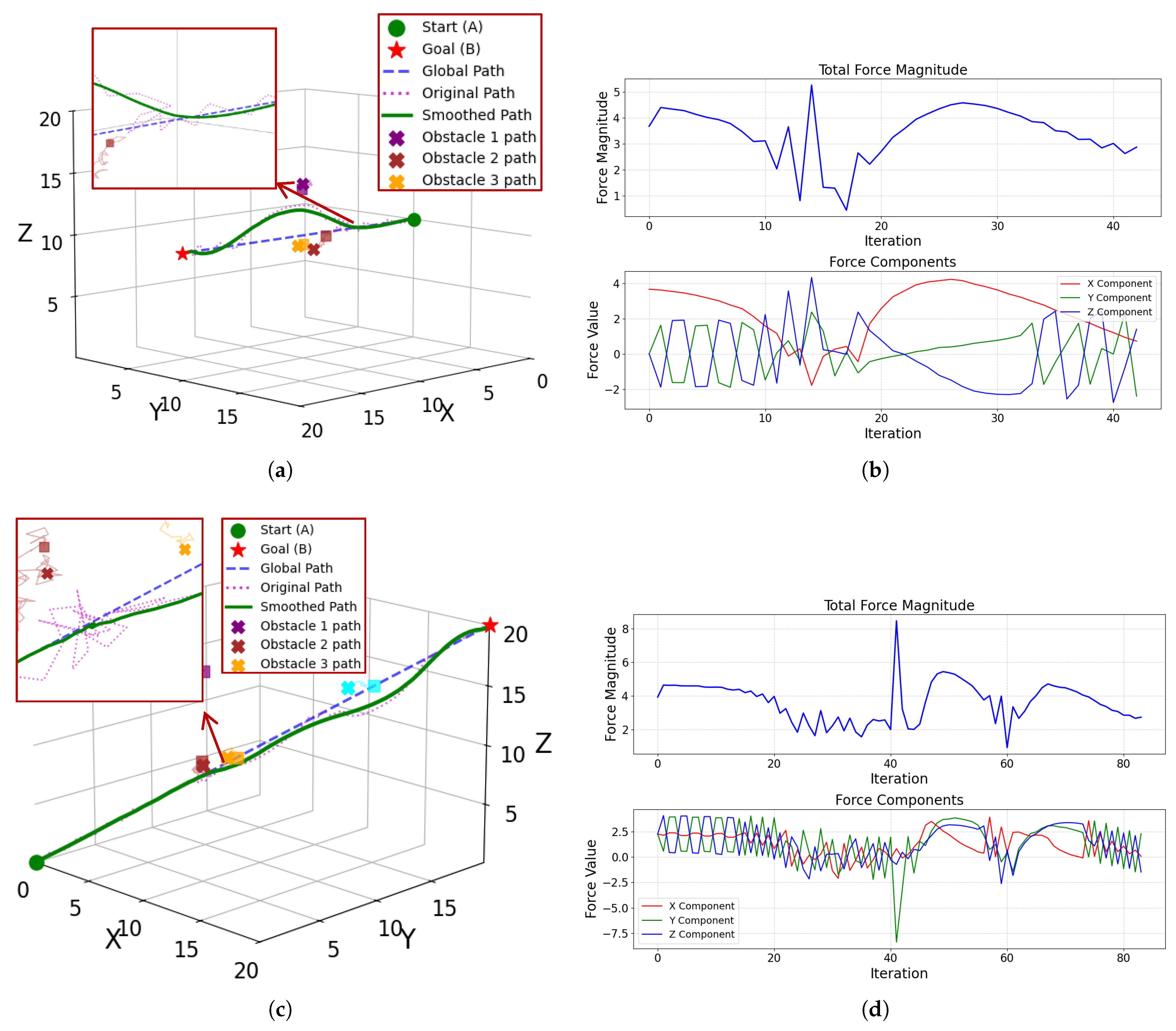
To verify the ability of the improved APF algorithm to avoid sudden threats in path planning within sub-airspaces, this study designed two guided path schemes for experimentation. The experimental results are shown in Figure 20, where green dots indicate the starting point, red stars indicate the ending point, blue dashed lines represent the guided within the subspace, purple dashed lines represent the original path without smoothing, and green solid lines represent the final generated real path. Three randomly moving obstacles were introduced into the experimental environment.
As shown in Figure 20a,c, under both guidance path schemes, the improved APF algorithm can effectively avoid sudden obstacles, achieving a 100% success rate in dynamic obstacle avoidance. Analyzing the obstacle avoidance process, it can be seen that the original path (purple dashed line) exhibits local abrupt changes due to the interference of obstacles. However, the real path (green solid line) after smooth optimization eliminates path abrupt changes by dynamically adjusting the balance between attractive and repulsive fields, generating a smooth and continuous path that satisfies the kinematic constraints of the UAV. Furthermore, the force variation curves in Figure 20b,d during the algorithm’s operation further verify that the comprehensive force field can achieve dynamic balance and eventually converge.

3.4. Collaborative Path Planning

Based on the verification results of the improved A* algorithm and APF algorithm in Section 3.2 and Section 3.3, this section focuses on verifying the comprehensive performance of collaborative path planning among sub-airspaces and real-time obstacle avoidance in sub-airspaces in static and dynamic threat scenarios under the sliding window guidance mechanism. The experimental results are shown in Figure 21 and Figure 22. The blue grid points in the figure identify the key nodes in the subspace inter-path planning; the local amplified area shows a specific subspace affected by sudden obstacles (represented by yellow grids). The green dotted line in this subspace represents the guidance path provided by the global planning, and the blue node is the obstacle avoidance path generated in real time based on local information. Among them, the three sub-graphs of Figure 21 correspond to the path planning result diagrams of t = 00:25:00, t = 00:28:15 and t = 00:33:15, respectively; the three sub-graphs of Figure 22 correspond to the path planning result diagrams of t = 00:29:00, t = 00:32:45 and t = 00:36:15, respectively.
The spatio-temporal data of high-threat scene path planning are shown in Table 6. In this verification, the flight control cycle for UAV path planning among sub-airspaces is set to 1 min (i.e., update the flight command according to the global path every 60 s), while the flight control period for real-time obstacle avoidance in the sub-airspace is 3 s (i.e., update the obstacle avoidance instruction every 3 s according to local sensor perception information and APF algorithm). In the experiment, sub-airspaces (23, 24, 23) and (24, 24, 24) triggered real-time path planning due to sudden threats. The verification results show that the collaborative path planning method proposed in this paper can effectively respond to emergencies, generate smooth obstacle avoidance paths, and ultimately ensure that the UAV reaches the target safely.

4. Discussion

This paper proposes an innovative solution to the challenging problem of UAV path planning in threatening environments.
In theory: A global subdivided grid system is constructed that integrates the advantages of Geosot binary coding and BeiDou grid location code subdivision rules, supporting multi-scale spatio-temporal data organization.
In terms of algorithms: An improved A*-APF hybrid architecture is designed, which enhances search efficiency through dynamic neighborhood search, resolves dead zones with a local backtracking mechanism, and achieves seamless switching between global and local planning through a sliding window-driven path association model.
In terms of performance: In ground threat scenarios and maze scenarios, our method outperforms traditional algorithms in comprehensive indicators such as path length, time consumption, and threat avoidance, and demonstrates robustness in handling dynamic and sudden threats.
Future work will extend to multi-UAV cooperative planning in complex threat scenarios, further optimizing the balance between real-time performance and energy consumption.

Author Contributions

Conceptualization, L.L. and L.R.; methodology, L.L. and L.R.; software, L.L. and L.R.; validation, L.L. and W.W.; formal analysis, L.L. and S.L.; investigation, L.L. and W.W.; resources, L.L. and H.X.; data curation, L.L. and R.Z.; writing—original draft preparation, L.L. and L.R.; writing—review and editing, L.L. and W.W.; visualization, L.L. and Z.Z.; supervision, L.L.; project administration, L.L. and S.L.; funding acquisition, L.R. All authors have read and agreed to the published version of the manuscript.

Funding

This research received no external funding.

Data Availability Statement

All data are included in the article.

Acknowledgments

The authors thank the editor and anonymous reviewers for their helpful comments on improving the quality of this article. They would also like to thank their laboratory team members for the technical support.

Conflicts of Interest

The authors declare no conflicts of interest.

References

  1. Jun, M.; D’Andrea, R. Path planning for unmanned aerial vehicles in uncertain and adversarial environments. In Cooperative Control: Models, Applications and Algorithms; Springer: Boston, MA, USA, 2003; pp. 95–110. [Google Scholar] [CrossRef]
  2. Liu, Y.; Zhang, X.; Guan, X.; Delahaye, D. Potential odor intensity grid based UAV path planning algorithm with particle swarm optimization approach. Math. Probl. Eng. 2016, 2016, 7802798. [Google Scholar] [CrossRef]
  3. Panov, A.I.; Yakovlev, K.S.; Suvorov, R. Grid path planning with deep reinforcement learning: Preliminary results. Procedia Comput. Sci. 2018, 123, 347–353. [Google Scholar] [CrossRef]
  4. Koay, T.B.; Chitre, M. Energy-efficient path planning for fully propelled AUVs in congested coastal waters. In Proceedings of the 2013 MTS/IEEE OCEANS-Bergen, Bergen, Norway, 10–14 June 2013; pp. 1–9. [Google Scholar] [CrossRef]
  5. Han, B.; Qu, T.; Tong, X.; Jiang, J.; Zlatanova, S.; Wang, H.; Cheng, C. Grid-optimized UAV indoor path planning algorithms in a complex environment. Int. J. Appl. Earth Obs. Geoinf. 2022, 111, 102857. [Google Scholar] [CrossRef]
  6. Sun, G.; Xu, Q.; Zhang, G.; Qu, T.; Cheng, C.; Deng, H. An Intelligent UAV Path-Planning Method Based on the Theory of the Three-Dimensional Subdivision of Earth Space. ISPRS Int. J. Geo-Inf. 2023, 12, 397. [Google Scholar] [CrossRef]
  7. Deng, C.; Cheng, C.; Qu, T.; Li, S.; Chen, B. A Method for Managing ADS-B Data Based on a 4D Airspace-Temporal Grid (GeoSOT-AS). Aerospace 2023, 10, 217. [Google Scholar] [CrossRef]
  8. Cao, J.; Shi, S.; Guo, Q.; Huang, G. Building Space Coding Based on Beidou Grid Position Code. Mob. Networks Appl. 2022, 27, 1700–1715. [Google Scholar] [CrossRef]
  9. Dijkstra, E.W. A note on two problems in connexion with graphs. In Edsger Wybe Dijkstra: His Life, Work, and Legacy; ACM Digital Library: New York, NY, USA, 2022; pp. 287–290. [Google Scholar] [CrossRef]
  10. Hart, P.E.; Nilsson, N.J.; Raphael, B. A formal basis for the heuristic determination of minimum cost paths. IEEE Trans. Syst. Sci. Cybern. 1968, 4, 100–107. [Google Scholar] [CrossRef]
  11. Noreen, I.; Khan, A.; Habib, Z. Optimal path planning using RRT* based approaches: A survey and future directions. Int. J. Adv. Comput. Sci. Appl. 2016, 7. [Google Scholar] [CrossRef]
  12. Holland, J.H. Genetic algorithms. Sci. Am. 1992, 267, 66–73. [Google Scholar] [CrossRef]
  13. Fox, D.; Burgard, W.; Thrun, S. The dynamic window approach to collision avoidance. IEEE Robot. Autom. Mag. 1997, 4, 23–33. [Google Scholar] [CrossRef]
  14. Khatib, O. Real-time obstacle avoidance for manipulators and mobile robots. Int. J. Robot. Res. 1986, 5, 90–98. [Google Scholar] [CrossRef]
  15. Yang, R.; Cheng, L. Path planning of restaurant service robot based on a-star algorithms with updated weights. In Proceedings of the 2019 12th International Symposium on Computational Intelligence and Design, Hangzhou, China, 14–15 December 2019; Volume 1, pp. 292–295. [Google Scholar] [CrossRef]
  16. Han, Z.; Chen, M.; Zhu, H.; Wu, Q. Ground threat prediction-based path planning of unmanned autonomous helicopter using hybrid enhanced artificial bee colony algorithm. Def. Technol. 2024, 32, 1–22. [Google Scholar] [CrossRef]
  17. Zhou, Z.; Guo, Y.; Wang, Y.; Lyu, J.; Gong, H.; Ye, X.; Li, Y. Multi-UAV Trajectory Optimization Under Dynamic Threats: An Enhanced GWO Algorithm Integrating a Priori and Real-Time Data. Int. J. Comput. Intell. Syst. 2025, 18, 1–21. [Google Scholar] [CrossRef]
  18. Zhang, M.; Su, C.; Liu, Y.; Hu, M.; Zhu, Y. Unmanned aerial vehicle route planning in the presence of a threat environment based on a virtual globe platform. ISPRS Int. J. Geo-Inf. 2016, 5, 184. [Google Scholar] [CrossRef]
  19. Li, W. An improved artificial potential field method based on chaos theory for UAV route planning. In Proceedings of the 2019 34th Youth Academic Annual Conference of Chinese Association of Automation, Jinzhou, China, 6–9 June 2019; pp. 47–51. [Google Scholar] [CrossRef]
  20. Chen, Z.; Xu, B. AGV path planning based on improved artificial potential field method. In Proceedings of the 2021 IEEE International Conference on Power Electronics, Computer Applications, Shenyang, China, 22–24 January 2021; pp. 32–37. [Google Scholar] [CrossRef]
  21. Lu, S.; Li, E.; Guo, R. An obstacles avoidance algorithm based on improved artificial potential field. In Proceedings of the 2020 IEEE International Conference on Mechatronics and Automation, Beijing, China, 13–16 October 2020; pp. 425–430. [Google Scholar] [CrossRef]
  22. Hu, H.; Liu, M.; Zhong, J.; Deng, X.; Cao, Y.; Fang, P. A Case Study of the 3D Water Vapor Tomography Model Based on a Fast Voxel Traversal Algorithm for Ray Tracing. Remote Sens. 2021, 13, 2422. [Google Scholar] [CrossRef]
  23. Chao, D.O.; Zhang, Y.; Ji, Z.; Li, Y.; Zhang, L.; Wu, Q. Three-dimension collision-free path planning of UAVs based on ADS-B information in low-altitude urban airspace. Chin. J. Aeronaut. 2025, 38, 103170. [Google Scholar] [CrossRef]
  24. He, X.; He, F.; Li, L.; Zhang, L.; Xiao, G. A route network planning method for urban air delivery. Transp. Res. Part E Logist. Transp. Rev. 2022, 166, 102872. [Google Scholar] [CrossRef]
  25. Jones, M.; Djahel, S.; Welsh, K. Path-planning for unmanned aerial vehicles with environment complexity considerations: A survey. ACM Comput. Surv. 2023, 55, 1–39. [Google Scholar] [CrossRef]
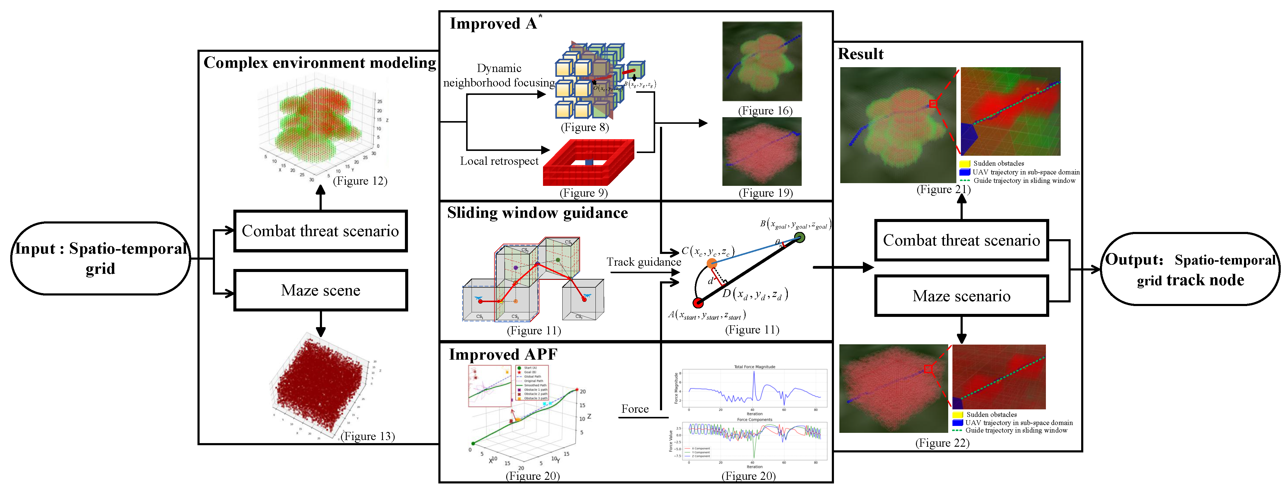
Figure 1. Research scheme of A*-APF path planning based on spatio-temporal grid optimization.
Drones 09 00661 g001
Figure 2. Actual shapes of spatial grid.
Drones 09 00661 g002
Figure 3. Three-dimensional coding conversion example.
Drones 09 00661 g003
Figure 4. Schematic diagram of time granularity subdivision relative to time reference layer.
Drones 09 00661 g004
Figure 5. Scenario and spatio-temporal grid division.
Drones 09 00661 g005
Figure 6. Ground threat unit modeling diagram: (a) vertical division; (b) horizontal division.
Drones 09 00661 g006
Figure 7. Basic neighborhood direction: (a) eight neighborhoods; (b) six neighborhoods; (c) four neighborhoods; (d) twenty-six neighborhoods.
Drones 09 00661 g007
Figure 8. Principle diagram of dynamic focusing neighborhood direction: (a) Plane π parallel to coordinate axes (9 neighbors); (b) Plane π parallel to face diagonals (9 neighbors); (c) Plane π parallel to body diagonal (19 neighbors).
Drones 09 00661 g008
Figure 9. UAV field of view model with adaptive zoom capability.
Drones 09 00661 g009
Figure 10. Design of transitional path in sub-airspace.
Drones 09 00661 g010
Figure 11. Sliding window and path guidance: (a) design of sliding window among sub-airspaces; (b) schematic diagram of path guidance in sub-airspace.
Drones 09 00661 g011
Figure 12. Ground threat scenario: (a) low-threat scenario; (b) high-threat scenario.
Drones 09 00661 g012
Figure 13. Maze scenario: (a) low-density maze; (b) low-aggregation maze; (c) high-density maze; (d) high-aggregation maze.
Drones 09 00661 g013
Figure 14. Planning results of different algorithms in low-level threat scenarios: (a) Improved A*; (b) Traditional A*; (c) GA; (d) SA; (e) Q-learning.
Drones 09 00661 g014
Figure 15. Planning results of different algorithms in medium-level threat scenarios: (a) Improved A*; (b) Traditional A*; (c) GA; (d) SA; (e) Q-learning.
Drones 09 00661 g015
Figure 16. Planning results of different algorithms in high-level threat scenarios: (a) Improved A*; (b) Traditional A*; (c) GA; (d) SA; (e) Q-learning.
Drones 09 00661 g016
Figure 17. Planning results of different algorithms in maze scenarios with ρ = 0.2 : (a) Improved A*; (b) Traditional A*; (c) GA; (d) SA; (e) Q-learning.
Drones 09 00661 g017
Figure 18. Planning results of different algorithms in maze scenarios with ρ = 0.5 : (a) Improved A*; (b) Traditional A*; (c) GA; (d) SA; (e) Q-learning.
Drones 09 00661 g018
Figure 19. Planning results of different algorithms in maze scenarios with ρ = 0.8 : (a) Improved A*; (b) Traditional A*; (c) GA; (d) SA; (e) Q-learning.
Drones 09 00661 g019
Figure 20. Path planning using improved APF algorithm in sub-airspace: (a) obstacle avoidance effect diagram of guidance path 1; (b) force curve diagram of guidance path 1; (c) obstacle avoidance effect diagram of guidance path 2; (d) force curve diagram of guidance path 2.
Drones 09 00661 g020
Figure 21. Collaborative path planning result diagram for high-threat scenarios: (a) t = 00:25:00; (b) t = 00:28:15; (c) t = 00:33:15.
Drones 09 00661 g021
Figure 22. Collaborative path planning result diagram for high-density maze scenarios: (a) t = 00:29:00; (b) t = 00:32:45; (c), t = 00:36:15.
Drones 09 00661 g022
Table 1. Grid information among sub-airspaces.
LongitudeLatitudeAltitude
Starting point110.000°25.000°0 m
Ending point110.042°25.042°3000 m
Grid size150 m150 m100 m
Table 2. Performance comparison of different algorithms in ground threat scenarios.
AlgorithmPerformance MetricsThreat Scenarios
Low-LevelMedium-LevelHigh-Level
Improved A*Path length (m)7215.697008.397422.98
Time (s)4.837.998.85
Total threat4.734.736.31
Search nodes18,90922,35333,290
Traditional A*Path length (m)8089.118098.118098.11
Time (s)18.1221.0242.85
Total threat6.316.3114.54
Search nodes52,94564,82386,554
GAPath length (m)8818.658871.409255.64
Time (s)5.829.1210.02
Total threat9.5010.1512.38
SAPath length (m)8180.268275.648344.28
Time (s)6.239.5611.09
Total threat9.5312.5213.92
Q-learningPath length (m)9764.6210,017.8610,709.81
Time (s)30.1032.9034.50
Total threat4.986.3811.07
Table 3. Performance comparison of different algorithms in maze scenarios.
AlgorithmPerformance MetricsObstacle Density ( ρ )
ρ = 0 . 2 ρ = 0 . 5 ρ = 0 . 8
Improved A*Path length (m)6878.717104.107990.92
Time (s)0.150.340.51
Total threat0.000.000.00
Search nodes559910,95312,993
Traditional A*Path length (m)8190.528645.708701.37
Time (s)0.230.481.32
Total threat0.000.000.00
Search nodes10,07823,00131,183
GAPath length (m)7974.558636.209505.45
Time (s)0.891.631.98
Total threat0.000.000.00
SAPath length (m)7346.157835.7010,016.26
Time (s)20.9023.8225.76
Total threat0.000.000.00
Q-learningPath length (m)9236.201015.0510,484.05
Time (s)30.1031.8733.50
Total threat0.000.000.00
Table 4. Performance comparison with the traditional A* algorithm.
Threat ScenarioPath LengthComputation TimePath Threat ValueNumber of Search Nodes
Low-threat10.90%73.34%25.04%64.29%
Medium-threat13.46%61.99%8.24%65.52%
High-threat8.34%79.35%56.60%61.54%
Table 5. Performance comparison with other intelligent algorithms.
Threat ScenarioIndexComparison with
GASAQ-Learning
Low-threatPath Length18.18%11.79%26.10%
Computation Time17.01%22.47%83.95%
Path Threat Value50.21%50.37%3.01%
Medium-threatPath Length21.00%15.31%30.04%
Computation Time12.39%16.42%75.71%
Path Threat Value42.86%53.75%9.25%
High-threatPath Length19.80%11.04%30.69%
Computation Time11.67%20.20%74.35%
Path Threat Value49.03%54.67%43.00%
Table 6. Spatio-temporal data table for collaborative path planning in high-threat scenarios.
Group 1Group 2Group 3Group 4
Spatial NodeTimestampSpatial NodeTimestampSpatial NodeTimestampSpatial NodeTimestamp
(0,0,0)00:00:00(19,23,19)00:25:00(33,24,23): (13,7,13)00:26:06(24,24,24): (10,15,9)00:27:21
(0,1,1)00:01:00(20,23,20)00:26:00(33,24,23): (14,7,14)00:26:09(24,24,24): (11,15,9)00:27:24
(0,2,2)00:02:00(21,23,21)00:24:00(33,24,23): (15,7,15)00:26:12(24,24,24): (11,15,10)00:27:27
(0,3,3)00:03:00(22,23,22)00:25:00(33,24,23): (15,8,15)00:26:15(24,24,24): (12,16,10)00:27:30
(0,4,4)00:04:00(23,24,23): (0,0,0)00:25:03(33,24,23): (16,8,16)00:26:18(24,24,24): (13,16,11)00:27:33
(0,5,5)00:05:00(23,24,23): (1,0,1)00:25:06(33,24,23): (17,8,17)00:26:21(24,24,24): (13,17,12)00:27:36
(0,6,6)00:06:00(23,24,23): (1,1,1)00:25:09(33,24,23): (17,9,17)00:26:24(24,24,24): (14,17,12)00:27:39
(1,7,7)00:07:00(23,24,23): (1,1,2)00:25:12(33,24,23): (18,9,18)00:26:27(24,24,24): (14,17,13)00:27:42
(2,8,8)00:08:00(23,24,23): (2,1,2)00:25:15(33,24,23): (19,9,19)00:26:30(24,24,24): (14,17,14)00:27:45
(3,9,9)00:09:00(23,24,23): (3,1,3)00:25:18(24,24,24): (0,9,0)00:26:33(24,24,24): (14,17,15)00:27:48
(4,10,10)00:10:00(23,24,23): (3,2,3)00:25:21(24,24,24): (1,0,1)00:26:36(24,24,24): (15,17,15)00:27:51
(5,11,11)00:11:00(23,24,23): (4,2,4)00:25:24(24,24,24): (1,1,1)00:26:59(24,24,24): (15,18,16)00:27:54
(6,12,12)00:12:00(23,24,23): (5,2,4)00:25:27(24,24,24): (2,1,1)00:26:42(24,24,24): (15,18,17)00:27:57
(7,13,13)00:13:00(23,24,23): (6,3,5)00:25:30(24,24,24): (3,1,1)00:26:45(24,24,24): (16,18,17)00:28:00
(8,13,14)00:14:00(23,24,23): (7,3,5)00:25:33(24,24,24): (3,1,2)00:26:48(24,24,24): (16,18,18)00:28:03
(9,13,15)00:15:00(23,24,23): (8,3,5)00:25:36(24,24,24): (3,1,2)00:26:51(24,24,24): (17,18,18)00:28:06
(10,14,16)00:16:00(23,24,23): (8,3,6)00:25:39(24,24,24): (3,1,3)00:26:54(24,24,24): (17,19,18)00:28:09
(11,15,17)00:17:00(23,24,23): (9,3,6)00:25:42(24,24,24): (3,1,3)00:26:57(24,24,24): (18,19,19)00:28:12
(12,16,17)00:18:00(23,24,23): (9,4,6)00:25:45(24,24,24): (4,1,4)00:27:00(24,24,24): (19,19,19)00:28:15
(13,17,17)00:19:00(23,24,23): (10,4,7)00:25:48(24,24,24): (4,1,4)00:27:03(25,25,25)00:29:15
(14,18,17)00:20:00(23,24,23): (11,4,8)00:25:51(24,24,24): (5,1,4)00:27:06(26,26,26)00:30:15
(15,19,17)00:21:00(23,24,23): (12,5,10)00:25:54(24,24,24): (6,15,8)00:27:09(27,27,27)00:31:15
(16,20,17)00:22:00(23,24,23): (12,6,11)00:25:57(24,24,24): (7,15,8)00:27:12(28,28,28)00:32:15
(17,21,17)00:23:00(23,24,23): (13,6,12)00:26:00(24,24,24): (8,15,9)00:27:15(29,29,29)00:33:15
(18,22,18)00:24:00(23,24,23): (13,6,13)00:26:03(24,24,24): (9,15,9)00:27:18--
Disclaimer/Publisher’s Note: The statements, opinions and data contained in all publications are solely those of the individual author(s) and contributor(s) and not of MDPI and/or the editor(s). MDPI and/or the editor(s) disclaim responsibility for any injury to people or property resulting from any ideas, methods, instructions or products referred to in the content.