Cluster Characteristics Analysis of UAV Air-to-Air Channels Based on Ray Tracing and Wasserstein Generative Adversarial Network with Gradient Penalty

Abstract

Air-to-air (A2A) communication plays a vital role in low-altitude unmanned aerial vehicle (UAV) networks and demands accurate channel modeling to support system analysis and design. A key challenge in A2A channel modeling lies in extracting reliable cluster characteristics, which are often limited due to the scarcity of measurement data. To overcome this limitation, a cluster characteristic analysis method is proposed for UAV A2A channels in built-up environments. First, we reconstruct virtual urban environments, followed by the acquisition of A2A channel data using ray tracing (RT) techniques. Then, a kernel power density (KPD) clustering algorithm is applied to group the multipath components (MPCs). To enhance the modeling accuracy of intra-cluster angular offsets in both elevation and azimuth domains, a Wasserstein generative adversarial network with gradient penalty (WGAN-GP) is further introduced for generative modeling. A comprehensive analysis is conducted on key cluster characteristics, including the intra-cluster number of MPCs, intra-cluster delay and angular spreads, number of clusters, and angular distributions. The numerical results demonstrate that the proposed WGAN-GP-based approach achieves superior angular fitting accuracy compared to conventional empirical distribution methods.

1. Introduction

The low-altitude economy is an integrated economic model driven primarily by the low-altitude flight activities of various types of aerial vehicles, promoting coordinated development across multiple sectors. In recent years, with the rapid advancement of the low-altitude economy, the deployment and application scenarios of unmanned aerial vehicles (UAVs) in urban airspace have become increasingly diverse, placing higher demands on efficient and reliable airborne communication capabilities [1,2,3,4,5]. These requirements are particularly critical for low-altitude UAV swarms, which are increasingly employed in collaborative search and rescue, multi-drone urban surveillance, distributed aerial sensing, and emergency response networks. As a core communication paradigm, air-to-air (A2A) communication plays a vital role in establishing robust UAV communication networks [6,7,8]. Consequently, A2A channel modeling has attracted growing attention, particularly under complex low-altitude built-up area propagation environments. Meanwhile, extensive channel measurement campaigns have demonstrated that multipath components (MPCs) tend to exhibit clustered structures in practical environments [9,10,11]. Cluster-based channel modeling not only improves modeling accuracy but also effectively reduces system complexity [12]. Therefore, an in-depth analysis of cluster characteristics, including angle and delay, is of significant theoretical and practical importance for enhancing the accuracy and applicability of A2A channel modeling.

The concept of path clusters, which refers to grouping MPCs with similar propagation characteristics, has been widely adopted in standardized and mainstream channel models such as COST 2100 [13], 3GPP TR 36.777 [14], and geometry-based stochastic channel models (GBSMs) [15,16]. Recent efforts have been made toward the modeling of cluster-based A2A channels. In [17], an extended three-dimensional (3D) ellipsoidal framework was introduced to describe far clusters induced by high-rise buildings and other dominant scattering objects. A cylindrical geometry was utilized in [18] to characterize static and dynamic clusters near the transmitter (Tx) and receiver (Rx), including local and remote clusters. In [19], a sub-terahertz cluster-based model was investigated using a 3D spherical structure, incorporating scattering fading effects caused by rough surfaces. Ref. [20] proposed an ellipsoidal geometry to describe the distribution of channel clusters and analyzed the impact of cluster distribution on the autocorrelation function. The authors of [21] investigated an A2A channel model considering specular reflection clusters and examined the influence of reflected paths on the channel based on measured data.

Machine learning has been increasingly applied in wireless propagation modeling due to its strength in handling complex data patterns [22,23]. In particular, clustering of MPCs has benefited from learning-based methods to improve modeling accuracy and flexibility. Recent studies have explored various clustering techniques. An entropy-based adaptive density clustering algorithm was introduced in [24] to enable efficient clustering analysis of terahertz channels. To mitigate noise effects, ref. [25] proposed a denoising framework based on a novel spatially transformed fuzzy C-means algorithm, validated through both simulations and measurements in a typical rural macro-cell scenario. The work in [26] studied static and dynamic cluster characteristics by clustering MPCs in an obstructed high-speed railway viaduct scenario. In [27], channel clustering was performed using a variational Bayesian Gaussian mixture model. A cluster-based UAV air-to-ground channel model was then developed, incorporating a four-state Markov chain to characterize cluster evolution. Using real-world measurement data at 6.5 GHz, ref. [28] applied the space-alternating generalized expectation maximization algorithm to estimate latent MPCs, followed by K-power-means (KPM) clustering for cluster characterization and tracking.

Overall, although the aforementioned studies have proposed novel and effective clustering algorithms, most of them primarily focus on terrestrial or indoor scenarios. Low-altitude UAV channels exhibit significant differences from conventional terrestrial channels, leading to distinct cluster characteristics. With the scarcity of measurement data, the cluster characteristics in A2A scenarios remain unclear, making channel modeling more challenging. Therefore, to address this research gap, this paper systematically extracts and analyzes key cluster parameters in A2A channels, thereby providing theoretical support for channel modeling and swarm communication network optimization. The main contributions and innovations are summarized as follows:

• A UAV A2A channel dataset is constructed for various representative built-up area scenarios using ray tracing (RT) simulations. An automatic clustering algorithm based on kernel power density (KPD) is applied to group MPCs, where the conventional Euclidean distance is replaced by the multipath component distance (MCD), resulting in more accurate clustering performance.
• In addition to providing empirical distribution expressions, a Wasserstein generative adversarial network with gradient penalty (WGAN-GP) is introduced to perform generative modeling of intra-cluster azimuth and elevation angle offsets using a large number of angular offset data.
• Based on the clustering results, the cluster characteristics of UAV A2A channels are systematically analyzed, including the number of sub-paths per cluster, the total number of clusters, intra-cluster delay and angular spreads, angular offsets, cluster Rician K-factor, and angular distributions. The numerical results demonstrate that the generated angular offset distributions closely match the RT data and outperform conventional empirical methods, validating the effectiveness of the generative model in improving modeling accuracy.

The remainder of this paper is organized as follows: Section 2 introduces the channel data generation method based on RT and the KPD clustering algorithm. Section 3 proposes the WGAN-GP framework. Section 4 presents a detailed analysis of cluster characteristics and compares the generated results with conventional empirical fitting results. Finally, conclusions are drawn in Section 5.

2. RT-Based Channel Data Acquisition and Clustering

2.1. UAV A2A Channel Description

A typical framework of a UAV A2A channel model in an urban scenario is illustrated in Figure 1. As UAVs fly over the city, various ground scatterers significantly affect wireless propagation [29,30]. In this A2A model, both the Tx and Rx are UAVs, and the communication link always contains a line-of-sight (LoS) component. Additionally, rooftop specular reflection (RSR) is considered [20], with all scatterers located below the UAVs. Each MPC is characterized by six parameters: azimuth angle of arrival (AAOA) ${\alpha }_i^{\mathrm{R}}$, elevation angle of arrival (EAOA) ${\beta }_i^{\mathrm{R}}$, azimuth angle of departure (AAOD) ${\alpha }_i^{\mathrm{T}}$, elevation angle of departure (EAOD) ${\beta }_i^{\mathrm{T}}$, delay ${\tau }_i$, and power $P_i$. These parameters are used to perform clustering of the MPCs. Clustering is motivated by the observation that, at a given time, many MPCs may share similar delay, angle, and so on, as they often originate from the same or closely located scatterers and arrive at the Rx in a superimposed manner. Since RSR components typically exhibit stronger power than non-line-of-sight (NLoS) components, the clustering analysis in this work focuses exclusively on the NLoS paths.

The NLoS channel impulse response (CIR) in A2A scenarios can be expressed as follows:

$$\begin{array}{cc}\hfill h_{n_m}^{\mathrm{NL}}(t,\tau ,{\alpha }^{\mathrm{T}},{\alpha }^{\mathrm{R}},{\beta }^{\mathrm{T}},{\beta }^{\mathrm{R}})=& \sum _{n=1}^{N\left(t\right)}\sum _{m=1}^{M\left(t\right)}\sqrt{P_{n_m}^{\mathrm{NL}}\left(t\right)}·e^{j{\mathsf{\Phi }}_{n_m}^{\mathrm{NL}}\left(t\right)}·\delta \left(\tau -{\tau }_n^{\mathrm{NL}}\left(t\right)-{\tau }_{n_m}^{\mathrm{NL}}\left(t\right)\right)\hfill \\ \hfill & \times \delta \left({\alpha }^{\mathrm{T}}-{\alpha }_n^{\mathrm{T}}\left(t\right)-{\alpha }_{n_m}^{\mathrm{T}}\left(t\right)\right)·\delta \left({\alpha }^{\mathrm{R}}-{\alpha }_n^{\mathrm{R}}\left(t\right)-{\alpha }_{n_m}^{\mathrm{R}}\left(t\right)\right)\hfill \\ \hfill & \times \delta \left({\beta }^{\mathrm{T}}-{\beta }_n^{\mathrm{T}}\left(t\right)-{\beta }_{n_m}^{\mathrm{T}}\left(t\right)\right)·\delta \left({\beta }^{\mathrm{R}}-{\beta }_n^{\mathrm{R}}\left(t\right)-{\beta }_{n_m}^{\mathrm{R}}\left(t\right)\right)\hfill \end{array}$$

(1)

where $N\left(t\right)$ denotes the time-varying number of clusters; $M\left(t\right)$ denotes the number of MPCs within each cluster; $P_{n_m}^{\mathrm{NL}}\left(t\right)$ and ${\mathsf{\Phi }}_{n_m}^{\mathrm{NL}}\left(t\right)$ represent the power and phase of the m-th sub-path in the n-th cluster, respectively; ${\tau }_n^{\mathrm{NL}}\left(t\right)$ and ${\tau }_{n_m}^{\mathrm{NL}}\left(t\right)$ denote the delay of the n-th cluster and the excess delay of its constituent MPCs, respectively; ${\alpha }_n^{\mathrm{T}}\left(t\right)$, ${\alpha }_n^{\mathrm{R}}\left(t\right)$, ${\beta }_n^{\mathrm{T}}\left(t\right)$, and ${\beta }_n^{\mathrm{R}}\left(t\right)$ denote the AAOD, AAOA, EAOD, and EAOA of the n-th cluster, respectively; ${\alpha }_{n_m}^{\mathrm{T}}\left(t\right)$, ${\alpha }_{n_m}^{\mathrm{R}}\left(t\right)$, ${\beta }_{n_m}^{\mathrm{T}}\left(t\right)$, and ${\beta }_{n_m}^{\mathrm{R}}\left(t\right)$ represent the corresponding excess angular offsets for each MPC within the cluster.

2.2. Scenario Setup and RT Simulation

In this work, RT simulations were conducted in various urban scenarios to obtain MPC datasets. RT is a deterministic modeling approach based on geometric optics and the uniform theory of diffraction. By importing detailed scenario models, the RT traced the propagation of rays emitted from the Tx until they reached the Rx, while capturing interactions such as reflection, diffraction, and scattering. This enabled the extraction of six-dimensional (6D) MPC parameters in UAV A2A environments. The size of each virtual urban scenario was 1000 m × 1000 m. Both the Tx and Rx UAVs were deployed in a grid pattern. The Tx UAVs were placed with a horizontal spacing of 100 m at an altitude of 150 m. The Rx UAVs were arranged with a horizontal spacing of 50 m, and their heights decreased from 140 m to 80 m in steps of 20 m. This arrangement allowed the UAVs to cover multiple regions within the simulation area. The detailed RT simulation parameters are summarized in

Table 1. The simulation details and parameters of RT.

Parameter	Value	Parameter	Value
Scenario	Suburban, urban, dense urban, urban high-rise	Tx altitude	150 m
Building area ratio	0.1, 0.3, 0.5, 0.5	Rx altitude	140 m, 120 m, 100 m, 80 m
Building density	750/km2, 500/km2, 300/km2, 300/km2	Frequency	2.4 GHz
Average building height	8 m, 15 m, 20 m, 50 m	Antenna type	Omnidirectional
Building width	11.6 m, 24.5 m, 40.8 m, 40.8 m	Transmit power	0 dBm
Street width	24.9 m, 20.2 m, 16.9 m, 16.9 m	Concrete	One-layer dielectric
Building location/height distribution	Uniform/Rayleigh distribution	Wet earth	Dielectric half-space

.

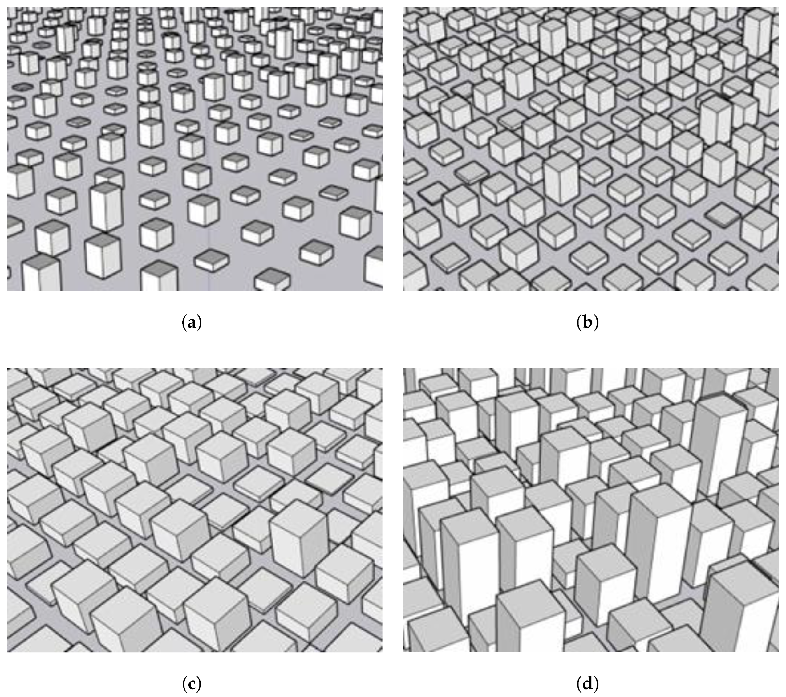
A 3D virtual city reconstruction method is introduced in this work to effectively reduce the complexity and cost of urban modeling while preserving essential environmental characteristics. Following International Telecommunication Union (ITU) recommendations, key scene features such as building area ratio, building density, and average building height were selected [31]. These extracted parameters were used to derive the configuration of the virtual city, enabling the construction of realistic 3D urban environments. Figure 2 illustrates four typical reconstructed urban scenarios. From suburban to urban high-rise, both building size and height increase progressively, demonstrating strong adaptability to various propagation environments. Simulations were conducted in these virtual urban scenarios.

2.3. KPD Clustering Algorithm

By simulating with RT, the 6D parameters of MPCs can be obtained. In practical wireless channel environments, MPCs typically exhibit a clustered structure, necessitating an effective clustering algorithm to group the MPCs accordingly. Traditional clustering algorithms, such as K-means and KPM, require the manual specification of the number of clusters. To address this, the KPD algorithm was employed, which is an automatic clustering method that identifies and clusters MPCs based on the analysis of data density distribution, thereby reducing dependence on user-defined parameters [32]. The main steps of the algorithm are as follows:

First, the distance between MPCs is calculated. For any given MPC sample $x_i$, its distance to other MPCs can be computed using the MCD metric [33]:

$${\mathrm{MCD}}_{i,j}=\sqrt{{∥{\mathrm{MCD}}_{i,j}^{\tau }∥}^2+{∥{\mathrm{MCD}}_{i,j}^{\mathrm{AOD}}∥}^2+{∥{\mathrm{MCD}}_{i,j}^{\mathrm{AOA}}∥}^2}$$

(2)

Here, ${\mathrm{MCD}}_{i,j}$ represents the distance between MPCs $x_i$ and $x_j$. The calculation methods for the delay and angular components are as follows:

$${\mathrm{MCD}}_{i,j}^{\tau }=\zeta ·{\displaystyle \frac{|{\tau }_i-{\tau }_j|}{\Delta {\tau }_{max}}}·{\displaystyle \frac{{\tau }_{\mathrm{std}}}{\Delta {\tau }_{max}}}$$

(3)

$${\mathrm{MCD}}_{i,j}^{\mathrm{AOA}/\mathrm{AOD}}={\displaystyle \frac{1}{2}}∥\left(\begin{array}{c}sin{\beta }_i^{\mathrm{R}/\mathrm{T}}cos{\alpha }_i^{\mathrm{R}/\mathrm{T}}\\ sin{\beta }_i^{\mathrm{R}/\mathrm{T}}sin{\alpha }_i^{\mathrm{R}/\mathrm{T}}\\ cos{\beta }_i^{\mathrm{R}/\mathrm{T}}\end{array}\right)-\left(\begin{array}{c}sin{\beta }_j^{\mathrm{R}/\mathrm{T}}cos{\alpha }_j^{\mathrm{R}/\mathrm{T}}\\ sin{\beta }_j^{\mathrm{R}/\mathrm{T}}sin{\alpha }_j^{\mathrm{R}/\mathrm{T}}\\ cos{\beta }_j^{\mathrm{R}/\mathrm{T}}\end{array}\right)∥$$

(4)

where $\Delta {\tau }_{max}$ and ${\tau }_{\mathrm{std}}$ represent the maximum delay difference and the standard deviation of the MPC delay, respectively, and $\zeta$ is the scaling factor.

For MPC $x_i$, the distances between it and all other MPC samples are computed and sorted in ascending order to obtain the separation distances $\Delta {\mathrm{MCD}}_i$. The calculation is given by

$$\Delta \mathrm{MC}{\mathrm{D}}_i=\left[\mathrm{MC}{\mathrm{D}}_{i,1},\mathrm{MC}{\mathrm{D}}_{i,2},\mathrm{MC}{\mathrm{D}}_{i,3},\dots ,\mathrm{MC}{\mathrm{D}}_{i,L-1}\right]$$

(5)

Here, L denotes the sum of the MPCs across all clusters. The initial value K is set to $\sqrt{L/2}$, and the first K separation distances of $\Delta {\mathrm{MCD}}_i$ are selected, denoted as $\Delta {\mathrm{MCD}}_i^K$. When the difference between adjacent values in $\Delta {\mathrm{MCD}}_i^K$, i.e., ${\mathrm{MCD}}_{i,j+1}-{\mathrm{MCD}}_{i,j}$, exceeds the threshold $\Delta d_{\mathrm{thresh}}$, the MPCs $x_{j+1}$ and $x_i$ are considered to belong to different clusters. Consequently, the value of K for $x_i$ is updated to j. The threshold is calculated as follows:

$$\Delta d_{\mathrm{thresh}}=\lambda ·max{\mathrm{MCD}}_{i,j}$$

(6)

where $\lambda$ denotes the scaling factor.

Using the above method, the K closest MPCs around the sample $x_i$ can be obtained, represented as the set $K_{x_i}$. A Gaussian kernel is applied in the delay domain, a Laplacian kernel in the angular domain, and an exponential kernel for power to calculate the density ${\rho }_{x_i}$.

$$\begin{array}{cc}\hfill {\rho }_{x_i}=\sum _{\begin{array}{c}{x}_j\in K_{x_i}\\ j\ne i\end{array}}& exp\left(P_j\right)·exp\left(-{\displaystyle \frac{|{\tau }_i-{\tau }_j{|}^2}{{\left({\sigma }_{\tau }\right)}^2}}\right)·exp\left(-{\displaystyle \frac{|{\alpha }_i^{\mathrm{T}}-{\alpha }_j^{\mathrm{T}}+k\pi |}{{\sigma }_{{\alpha }^{\mathrm{T}}}}}\right)·exp\left(-{\displaystyle \frac{|{\alpha }_i^{\mathrm{R}}-{\alpha }_j^{\mathrm{R}}+k\pi |}{{\sigma }_{{\alpha }^{\mathrm{R}}}}}\right)\hfill \\ \hfill & \times exp\left(-{\displaystyle \frac{|{\beta }_i^{\mathrm{T}}-{\beta }_j^{\mathrm{T}}|}{{\sigma }_{{\beta }^{\mathrm{T}}}}}\right)·exp\left(-{\displaystyle \frac{|{\beta }_i^{\mathrm{R}}-{\beta }_j^{\mathrm{R}}|}{{\sigma }_{{\beta }^{\mathrm{R}}}}}\right)\hfill \end{array}$$

(7)

where

$$k=\left\{\begin{array}{cc}2,\hfill & \mathrm{if}{\alpha }_i^{\mathrm{T}/\mathrm{R}}-{\alpha }_j^{\mathrm{T}/\mathrm{R}}\le -\pi \hfill \\ -2,\hfill & \mathrm{if}{\alpha }_i^{\mathrm{T}/\mathrm{R}}-{\alpha }_j^{\mathrm{T}/\mathrm{R}}\ge \pi \hfill \\ 0,\hfill & \mathrm{otherwise}\hfill \end{array}\right.$$

(8)

Here, ${\sigma }_{(·)}$ denotes the standard deviation operator.

To eliminate the impact of power differences between clusters on density and accurately identify cluster centroids, the MPC density for each MPC sample is normalized as follows:

$${\rho }_{x_i}^{\ast }={\displaystyle \frac{{\rho }_{x_i}}{{\displaystyle \underset{y\in K_{x_i}\cup \left\{x_i\right\}}{max}{\rho }_y}}}$$

(9)

MPCs with a relative density of 1 are considered the most influential within a cluster and are treated as cluster centroids. For each MPC $x_i$, if ${\rho }_{x_i}^{\ast }=1$, it is labeled as a key MPC, forming the set $\widehat{\Omega }=\left\{x_i|x_i\in \Omega ,{\rho }_{x_i}^{\ast }=1\right\}$. Key MPCs serve as the initial cluster centroids. For non-key MPCs with ${\rho }_{x_i}^{\ast }<1$, their high-density neighboring MPCs are defined as follows:

$${\overline{x}}_i=arg\underset{\begin{array}{c}{x}_j\in \Omega ,j\ne i,\\ {\rho }_{x_j}^{\ast }>{\rho }_{x_i}^{\ast }\end{array}}{min}{\mathrm{MCD}}_{i,j}$$

(10)

Among all MPCs, the MPC $x_j$ whose relative density satisfies ${\rho }_{x_j}^{\ast }>{\rho }_{x_i}^{\ast }$ and which has the smallest MCD to $x_i$ needs to be found. By connecting each MPC to its high-density neighboring MPC, a directed graph can be constructed.

$$G_1=\left(\Omega ,{\varsigma }_1\right)$$

(11)

The vertex set represents the complete set of MPCs, denoted as $\Omega$, while the edge set ${\varsigma }_1$ is defined as ${\varsigma }_1=\{x_i\to {\overline{x}}_i\mid x_i\in \Omega \setminus \widehat{\Omega }\}$. In addition, undirected edges are constructed between each MPC and its K nearest MPCs, resulting in an undirected graph.

$$G_2=\left(\Omega ,{\varsigma }_2\right)$$

(12)

The edge set ${\varsigma }_2$ can be represented as ${\varsigma }_2=\{x_i,x_j\mid x_i\in \Omega ,x_j\in K_{x_i}\}$. If there exists a path in $G_2$ connecting two key MPCs where all MPC nodes along the path have a relative density greater than a predefined threshold $\chi$, the clusters represented by these two key MPCs are merged into a single new cluster. A larger value of $\chi$ typically results in more clusters. Based on empirical analysis, a reasonable value is 0.8, as suggested in [34]. The pseudo-code of this algorithm is shown in Algorithm 1.

Algorithm 1 KPD Clustering Algorithm.

Require:  MPC parameter set $\mathcal{X}=\{x_1,x_2,\dots ,x_L\}$, each $x_i$ includes delay, angle and power Ensure:  Cluster assignments, cluster centroids 1:  for each $x_i\in \mathcal{X}$ do 2:        for each $x_j\in \mathcal{X},j\ne i$ do 3:              Compute $MC{D}_{i,j}$ 4:        end for 5:        Sort $MC{D}_{i,j}$ in ascending order 6:        Set initial neighbor number $K=\sqrt{L/2}$ 7:        Adjust K if distance increment $>\Delta d_{thresh}$ 8:  end for 9:  for each $x_i\in \mathcal{X}$ do 10:      Compute kernel density ${\rho }_{x_i}$ using K nearest neighbors 11:      Normalize density: ${\rho }_{x_i}^{\ast }={\rho }_{x_i}/{max}_{y\in K_{x_i}\cup \left\{x_i\right\}}{\rho }_y$ 12:      if ${\rho }_{x_i}^{\ast }=1$ then 13:            Mark $x_i$ as cluster centroid 14:      end if 15:  end for 16:  for each non-centroid $x_i$ do 17:        Link $x_i$ to nearest neighbor $x_j$ with ${\rho }_{x_j}^{\ast }>{\rho }_{x_i}^{\ast }$ 18:  end for 19:  Merge clusters if their centroids are connected through points with density greater than $\chi$ 20:  return Cluster assignments, cluster centroids

To objectively evaluate the effectiveness of the clustering algorithms employed in this work, we further compared the performance of the proposed method with several mainstream clustering algorithms, such as KPM. The clustering quality was quantitatively assessed using widely adopted metrics such as the Silhouette Coefficient and Calinski–Harabasz index, which primarily reflect the compactness, separability, and overlap of the clustering results [26,35]. Higher Silhouette Coefficient and Calinski–Harabasz index values generally indicate better clustering performance.

Table 2. Clustering performance comparison of the different algorithms.

Methods	Effectiveness Indexes
	Silhouette Coefficient	Calinski–Harabasz Index
KPD	0.71	311.94
K-means	0.55	245.77
KPM	0.66	262.77

presents the performance comparison results of the different clustering methods under these metrics. As shown in the table, the KPD algorithm not only achieves superior performance, but also does not require manual specification of the number of clusters, demonstrating better adaptability and practicality. These advantages make the method promising for further applications and extensions in future work.

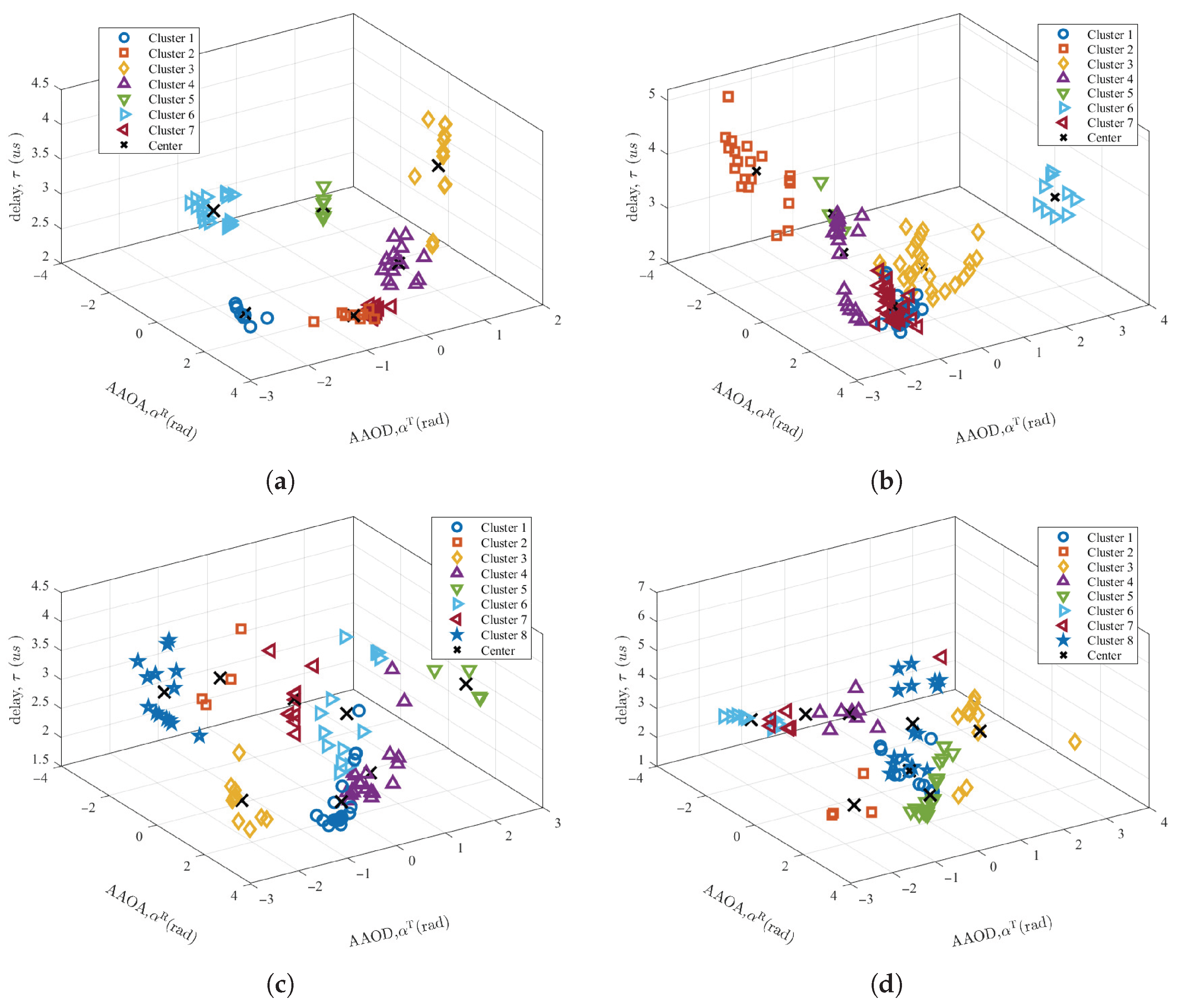
Figure 3 illustrates the clustering results of MPCs using the KPD algorithm in different scenarios. The results correspond to an exemplary configuration of buildings and a specific pair of Tx and Rx positions. Different clusters are distinguished by various colors and markers, while cluster centroids are indicated by black crosses. Effective clustering is observed in all four scenarios, with AAOA and AAOD showing similar angular spread ranges. From both the delay and angular domains, a large number of scattering clusters are evident in urban environments. As building density increases, the distribution of clusters becomes more dispersed. This is because the propagation environment in high-density urban areas with tall buildings is more complex. Buildings cause more frequent reflections, scatterings, and diffractions, leading to a more irregular spatial distribution of MPCs.

3. Empirical Fitting and Generation Method

3.1. Cluster Parameter and Distribution Fitting Methods

The cluster root mean square delay spread (RMS-DS) is used to quantify the temporal dispersion characteristics of MPCs within a cluster. It reflects the degree of temporal dispersion of the multipath signals. Similar to the intra-cluster delay spread (DS), the root mean square angular spread (RMS-AS) characterizes the statistical distribution of MPCs’ angles within a cluster in wireless channels. It reflects the extent of signal dispersion in the angular domain. Specifically, RMS-AS includes the azimuth angular spread of arrival (AAS), azimuth angular spread of departure (ADS), elevation angular spread of arrival (EAS), and elevation angular spread of departure (EDS). The calculation methods of DS and AS are as follows:

$${\sigma }_{\varsigma }=\sqrt{{\displaystyle \frac{{\displaystyle \sum _{c=1}^C}{\left({\varsigma }_c-{\varsigma }_{\mathrm{m}}\right)}^2{P}_c}{{\displaystyle \sum _{c=1}^C}{P}_c}}}$$

(13)

where C denotes the number of MPCs within the cluster, $P_c$ represent the power, $\varsigma \in \left\{\tau ,{\alpha }^{\mathrm{T}},{\alpha }^{\mathrm{R}},{\beta }^{\mathrm{T}},{\beta }^{\mathrm{R}}\right\}$ represents the delay and four types of angles, and ${\varsigma }_{\mathrm{m}}$ denotes the power-weighted mean delay or angle, calculated as follows:

$${\varsigma }_{\mathrm{m}}={\displaystyle \frac{{\displaystyle \sum _{c=1}^C}{\varsigma }_c{P}_c}{{\displaystyle \sum _{c=1}^C}{P}_c}}$$

(14)

The cluster K-factor is used to describe the ratio between the power of the dominant MPC and the total power of the remaining MPCs within a cluster. It is calculated as follows:

$$K=10·{log}_{10}\left({\displaystyle \frac{max\left(P_c\right)}{{\displaystyle \sum _{c=1}^C}{P}_c-max\left(P_c\right)}}\right)$$

(15)

Various standardized channel models such as 3GPP and WINNER commonly adopt specific probability density functions (PDFs), including the Gaussian [14], Laplace [36], and von Mises distributions [37], to characterize angular offset properties. Motivated by these practices, this work selected several widely used probabilistic models, namely, the normal, log-normal, Laplace, and von Mises distributions, to analyze the cluster characteristics. These distributions are widely applied in wireless channel modeling. The corresponding PDF expressions are presented as follows:

$$f\left(x\right)=\left\{\begin{array}{cc}{\displaystyle \frac{1}{\sqrt{2\pi }\sigma }}exp\left(-{\displaystyle \frac{{(x-\mu )}^2}{2{\sigma }^2}}\right),\hfill & \left(\mathrm{Normal}\right)\hfill \\ {\displaystyle \frac{1}{\sqrt{2\pi }x\sigma }}exp\left(-{\displaystyle \frac{{(lnx-\mu )}^2}{2{\sigma }^2}}\right),\hfill & x>0\left(\mathrm{Lognormal}\right)\hfill \\ {\displaystyle \frac{1}{2b}}exp\left(-{\displaystyle \frac{|x-\mu |}{b}}\right),\hfill & b>0\left(\mathrm{Laplace}\right)\hfill \\ {\displaystyle \frac{1}{2\pi I_0\left(\kappa \right)}}exp\left(\kappa cos(x-\mu )\right),\hfill & \kappa >0(\mathrm{Von}\mathrm{Mises})\hfill \end{array}\right.$$

(16)

where b is the scale parameter for the Laplace distribution (b > 0), $\kappa$ is the concentration parameter for the von Mises distribution ($\kappa$ > 0), and $I_0(·)$ denotes the modified Bessel function of the first kind and order zero.

3.2. WGAN-GP-Based Intra-Cluster Angle Generation

GANs are a type of adversarial neural network typically composed of a generator and a discriminator. The generator learns to produce data samples that approximate the real data distribution, while the discriminator aims to distinguish between real and generated samples. When the two networks reach a Nash equilibrium, the generator is capable of producing samples that are nearly indistinguishable from real data. Due to the diffuse reflection caused by rough surfaces, the angular offsets of MPCs within clusters are inherently random. Therefore, employing GANs to uncover the underlying statistical distribution of these angular offsets and subsequently generate random offsets is a practical and efficient approach. In this adversarial game, the generator G maps noise drawn from a prior distribution $P_{\mathit{z}}\left(\mathit{z}\right)$ to generate realistic samples $G\left(\mathit{z}\right)$ in an attempt to approximate the true data distribution $P_{\mathrm{data}}$. The discriminator D is responsible for distinguishing real samples ${\mathit{x}}_r\sim P_{\mathrm{data}}$ from generated samples. Both networks optimize the following min–max training objective:

$$\underset{G}{min}\underset{D}{max}{\mathbb{E}}_{{\mathit{x}}_r\sim P_{\mathrm{data}}}\left[logD\left({\mathit{x}}_r\right)\right]+{\mathbb{E}}_{\mathit{z}\sim P_{\mathit{z}}}\left[log\left(1-D\left(G\right(\mathit{z}\left)\right)\right)\right]$$

(17)

The above objective is equivalent to minimizing the Jensen–Shannon (JS) divergence between $P_{\mathrm{data}}$ and $P_{\mathit{z}}$. However, this often makes it difficult for the generator and discriminator to reach Nash equilibrium during adversarial training, which may result in issues such as training instability, vanishing gradients, and mode collapse, ultimately leading to a lack of diversity in the generated data. To address these problems, ref. [38] proposed the Wasserstein GAN, which introduces a new metric called the Wasserstein-1 distance, to measure the similarity between two probability distributions. This distance can be expressed as follows:

$$\mathcal{W}\left(P_{\mathrm{data}},P_g\right)=\underset{\gamma \in \mathsf{\Pi }(P_{\mathrm{data}},P_g)}{inf}{\mathbb{E}}_{({\mathit{x}}_r,{\mathit{x}}_g)\sim \gamma }\left[∥{\mathit{x}}_r-{\mathit{x}}_g∥\right]$$

(18)

Here, inf denotes the infimum, and $\mathsf{\Pi }\left(P_{\mathrm{data}},P_g\right)$ represents the set of all joint distributions $\gamma \left({\mathit{x}}_r,{\mathit{x}}_g\right)$ with marginals $P_{\mathrm{data}}$ and $P_g$. By employing the Kantorovich–Rubinstein duality, the objective function of WGAN can be derived as follows:

$$\underset{G}{min}\underset{f\in \mathcal{D}}{max}\left\{{\mathbb{E}}_{{\mathit{x}}_r\sim P_{\mathrm{data}}}\left[f\left({\mathit{x}}_r\right)\right]-{\mathbb{E}}_{\mathit{z}\sim P_{\mathit{z}}}\left[f\left(G\right(\mathit{z}\left)\right)\right]\right\}$$

(19)

where $\mathcal{D}$ is the set of 1-Lipschitz functions. WGAN has achieved improvements in training stability, but its performance can sometimes be unsatisfactory. This issue arises because the Lipschitz constraint imposed on the discriminator is enforced by weight clipping. To address this, ref. [39] introduced the gradient penalty as a replacement for weight clipping, resulting in the WGAN-GP. The loss functions for the discriminator and generator are defined as follows:

$${\mathcal{L}}_D=\underset{\mathrm{Original}\mathrm{critic}\mathrm{loss}}{\underbrace{{\mathbb{E}}_{{\mathit{x}}_g\sim P_g}\left[D\left({\mathit{x}}_g\right)\right]-{\mathbb{E}}_{{\mathit{x}}_r\sim P_{\mathrm{data}}}\left[D\left({\mathit{x}}_r\right)\right]}}+\underset{\mathrm{Gradient}\mathrm{penalty}}{\underbrace{\lambda {\mathbb{E}}_{\widehat{\mathit{x}}\sim P_{\widehat{\mathit{x}}}}\left[{\left({∥{\nabla }_{\widehat{\mathit{x}}}D\left(\widehat{\mathit{x}}\right)∥}_2-1\right)}^2\right]}}$$

(20)

$${\mathcal{L}}_G=-{\mathbb{E}}_{{\mathit{x}}_g\sim P_g}\left[D\left({\mathit{x}}_g\right)\right]$$

(21)

where parameter $\lambda$ denotes the weight of the gradient penalty; ∇ represents the gradient function; $\widehat{\mathit{x}}=\epsilon {\mathit{x}}_r+(1-\epsilon ){\mathit{x}}_g$, $\epsilon \sim U(0,1)$, i.e., $P_{\widehat{\mathit{x}}}$, represents the linear interpolation between the generated and real data samples. During training, the discriminator D and generator G are optimized alternately. Once convergence is achieved, the trained generator is extracted to reproduce the statistical distribution of intra-cluster angular offsets.

Our WGAN-GP-based framework for generating cluster angular offsets is illustrated in Figure 4 and consists of three main components: the discriminator network, the generator network, and the loss function module. First, intra-cluster information is extracted using the clustering algorithm, based on which the cluster angular offset data are computed. Then, the generator takes a 128-dimensional random noise vector as input, and through four fully connected layers (with 256, 512, 256, and 2 nodes, respectively), it progressively extracts features and outputs a two-dimensional (2D) vector representing the angular offset in the form of $(cos\theta ,sin\theta )$. These generated samples, together with RT data, are fed into the discriminator, which also comprises four fully connected layers (with 256, 512, 256, and 1 nodes, respectively). The discriminator takes a 2D vector as input and outputs a scalar value. The feedback from the discriminator is used to iteratively optimize both the generator and discriminator networks, refining the generated results to better match the angular offset data.

4. Numerical Results Analysis

The clustering analysis above provides cluster labels for each MPC and the total number of clusters. Subsequently, various cluster parameters were quantitatively analyzed, including the number of MPCs within each cluster, the total number of clusters, intra-cluster delay and angular spreads, intra-cluster angular offsets, cluster Rician K-factor, and the distributions of cluster azimuth and elevation angles.

Table 3. Scatterer cluster parameters in different urban scenarios.

Cluster Parameters	Statistical Distribution	Suburban	Urban	Dense Urban	Urban High-Rise
Number of intra-cluster MPCs	Log-normal	${\mu }_M=2.9489$	${\mu }_M=2.8288$	${\mu }_M=2.6663$	${\mu }_M=2.637$
		${\sigma }_M=0.7073$	${\sigma }_M=0.7107$	${\sigma }_M=0.6888$	${\sigma }_M=0.7458$
Cluster Rician K-factor (dB)	Normal	${\mu }_{KF}=-1.8687$	${\mu }_{KF}=-1.6384$	${\mu }_{KF}=-0.0867$	${\mu }_{KF}=1.8006$
		${\sigma }_{KF}=5.9163$	${\sigma }_{KF}=4.4894$	${\sigma }_{KF}=5.0372$	${\sigma }_{KF}=5.0738$
RMS-DS ($\mathsf{\mu }$s)	Log-normal	${\mu }_{DS}=-2.1744$	${\mu }_{DS}=-1.9138$	${\mu }_{DS}=-1.8707$	${\mu }_{DS}=-1.3559$
		${\sigma }_{DS}=1.4066$	${\sigma }_{DS}=1.0632$	${\sigma }_{DS}=1.0945$	${\sigma }_{DS}=1.0648$
RMS-AAS (rad)	Log-normal	${\mu }_{AAS}=-2.6266$	${\mu }_{AAS}=-2.4910$	${\mu }_{AAS}=-2.4662$	${\mu }_{AAS}=-2.3759$
		${\sigma }_{AAS}=1.1078$	${\sigma }_{AAS}=1.0239$	${\sigma }_{AAS}=1.1611$	${\sigma }_{AAS}=1.1854$
RMS-EAS (rad)	Log-normal	${\mu }_{EAS}=-3.2887$	${\mu }_{EAS}=-2.9729$	${\mu }_{EAS}=-2.9642$	${\mu }_{EAS}=-2.5757$
		${\sigma }_{EAS}=1.0810$	${\sigma }_{EAS}=1.1351$	${\sigma }_{EAS}=1.1686$	${\sigma }_{EAS}=0.9495$
RMS-ADS (rad)	Log-normal	${\mu }_{ADS}=-2.6185$	${\mu }_{ADS}=-2.3731$	${\mu }_{ADS}=-2.4322$	${\mu }_{ADS}=-2.3836$
		${\sigma }_{ADS}=1.1388$	${\sigma }_{ADS}=1.0399$	${\sigma }_{ADS}=1.1730$	${\sigma }_{ADS}=1.2551$
RMS-EDS (rad)	Log-normal	${\mu }_{EDS}=-3.3374$	${\mu }_{EDS}=-2.9844$	${\mu }_{EDS}=-2.9831$	${\mu }_{EDS}=-2.6509$
		${\sigma }_{EDS}=0.9841$	${\sigma }_{EDS}=0.9998$	${\sigma }_{EDS}=1.1204$	${\sigma }_{EDS}=0.9706$
AAOA offset (rad)	von Mises	${\mu }_{AAOA}=0.0006$	${\mu }_{AAOA}=0.0001$	${\mu }_{AAOA}=0.0013$	${\mu }_{AAOA}=-0.0002$
		${\kappa }_{AAOA}=16.0348$	${\kappa }_{AAOA}=18.4477$	${\kappa }_{AAOA}=14.6958$	${\kappa }_{AAOA}=9.6832$
AAOD offset (rad)	von Mises	${\mu }_{AAOD}=-0.0013$	${\mu }_{AAOD}=-0.0014$	${\mu }_{AAOD}=-0.0016$	${\mu }_{AAOD}=0.0041$
		${\kappa }_{AAOD}=13.3895$	${\kappa }_{AAOD}=15.1836$	${\kappa }_{AAOD}=12.9293$	${\kappa }_{AAOD}=9.2567$
EAOA offset (rad)	Laplace	${\mu }_{EAOA}=-0.011$	${\mu }_{EAOA}=-0.0151$	${\mu }_{EAOA}=-0.0140$	${\mu }_{EAOA}=-0.0315$
		$b_{EAOA}=0.0842$	$b_{EAOA}=0.1016$	$b_{EAOA}=0.1208$	$b_{EAOA}=0.1427$
EAOD offset (rad)	Laplace	${\mu }_{EAOD}=-0.0135$	${\mu }_{EAOD}=-0.0163$	${\mu }_{EAOD}=-0.0151$	${\mu }_{EAOD}=-0.0295$
		$b_{EAOD}=0.0818$	$b_{EAOD}=0.1012$	$b_{EAOD}=0.1203$	$b_{EAOD}=0.1554$

summarizes the statistical modeling results of these cluster characteristics. Detailed descriptions are given below.

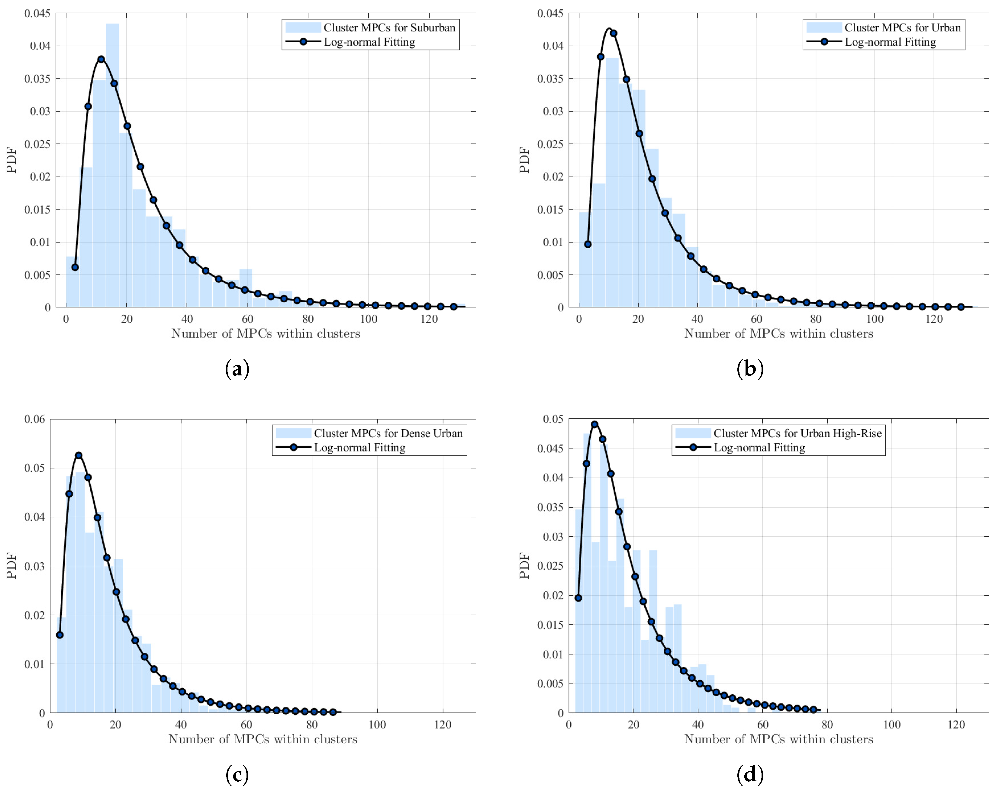
Figure 5 shows the statistical results of the number of MPCs per cluster. It can be observed that the log-normal distribution effectively modeled the number of MPCs within a cluster. Specifically, the natural logarithm of the number of MPCs per cluster followed a normal distribution with mean $\mu$ and variance ${\sigma }^2$, and the original expected value could be calculated from $exp\left(\mu +{\sigma }^2/2\right)$. In the suburban scenario, the mean and standard deviation were $2.9489$ and $0.70728$, respectively. The mean decreased gradually to $2.8288$, $2.6663$, and $2.637$ across the urban, dense urban, and urban high-rise scenarios, while the standard deviation remained around $0.7$. It is evident that the number of MPCs per cluster gradually decreased from suburban to high-rise urban environments. This trend is due to suburban areas featuring shorter and more numerous buildings, which provide abundant reflective surfaces within small areas. As building width and height increase, signal blockage effects become more pronounced and propagation directions become more dispersed, resulting in fewer MPCs per cluster after clustering.

The number of clusters reflects the richness of MPC clusters in the UAV A2A channel and depends on the communication environment. Across different scenarios, the number of clusters typically ranged from 3 to 10. From suburban to high-rise urban scenarios, the mean number of clusters gradually increased, which aligns with the analysis of the number of MPCs per cluster. High-rise urban areas had a stronger dispersive effect on signal propagation, which is also evident from the clustering results shown in Figure 3.

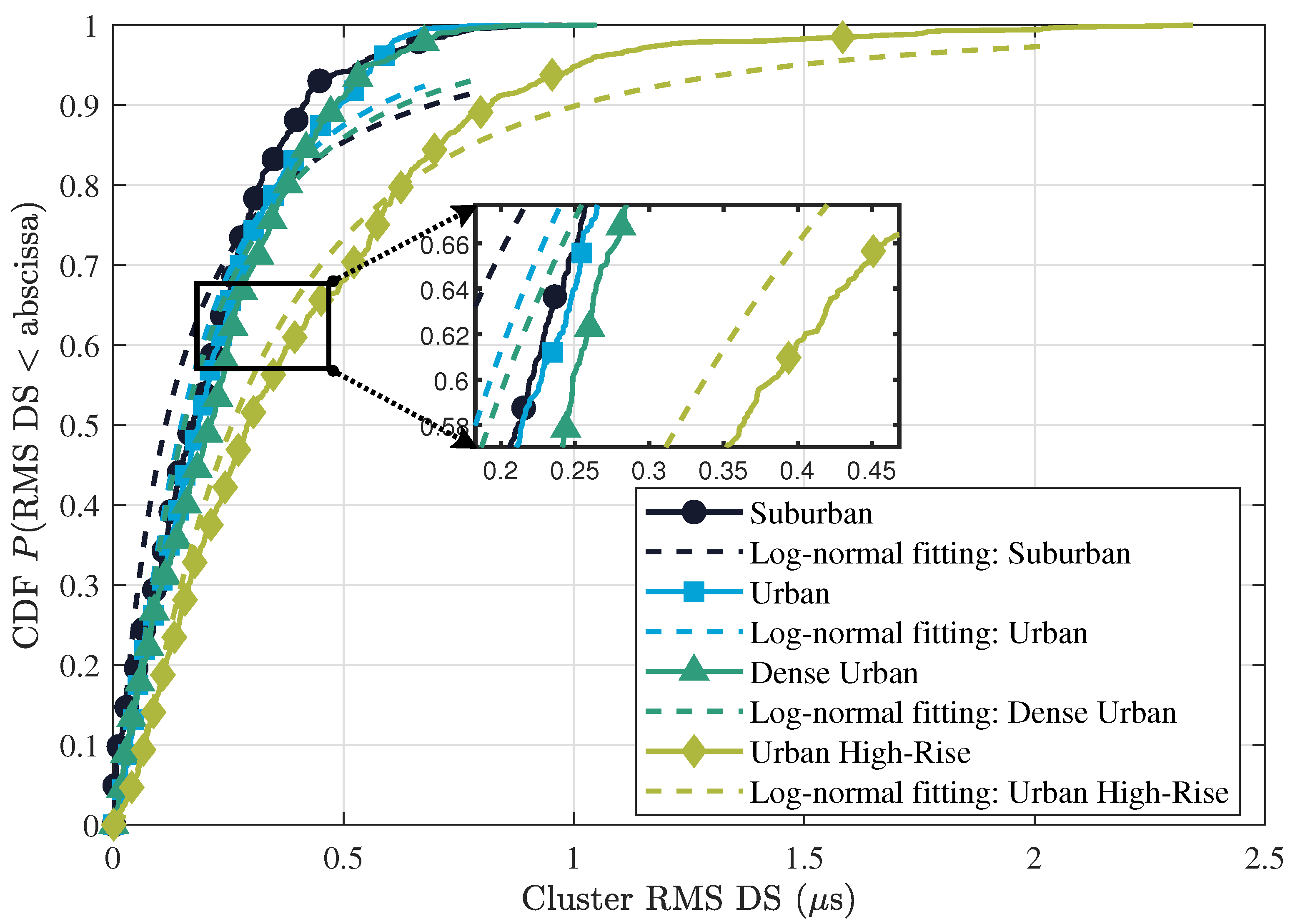
Figure 6 illustrates the cumulative distribution functions (CDFs) of cluster RMS-DS across different scenarios, along with their corresponding lognormal fitting results. It can be observed that the lognormal distribution provided a good fit for characterizing the statistical behavior of the RMS-DS. A magnified view of the x-axis range from 0.2 to 0.45 is presented to better reveal the differences across scenarios. From suburban to urban high-rise scenarios, the means of the lognormal distribution were −2.1744, −1.9138, −1.8707, and −1.3559, respectively, while the standard deviations were 1.4066, 1.0632, 1.0945, and 1.0648, respectively. It is evident that the RMS-DS increased progressively with building height, with a more pronounced growth observed in high-rise urban environments. This trend is attributed to the more dispersed intra-cluster multipath distribution in highly built-up environments, where complex building layouts introduce richer propagation paths and larger delay variations, ultimately resulting in increased delay spreads.

Figure 7 illustrates the CDFs of cluster RMS-ASs and their corresponding fitting results across four different scenarios. It can be observed that the RMS-ASs approximately followed a log-normal distribution, with detailed parameters listed in Table 3. The distributions of AAS and ADS within clusters were similar across scenarios, as were the EAS and EDS. For a given scenario, the fitted mean values of the azimuth angular spreads were larger than the elevation angular spreads. Moreover, both EAS and EDS showed an increasing trend from suburban to high-rise urban scenarios, which can be explained by the greater availability of vertical structures for reflection and scattering as building heights increase. Compared to the suburban scenario, where reflections are mainly concentrated at low elevations with an average building height of approximately 8 m, urban and high-rise urban environments offer effective reflection paths across multiple height layers, with average building heights around 20 and 50 m. This leads to a more dispersed multipath distribution in the elevation domain and consequently increases the cluster elevation angular spreads.

The intra-cluster angular offset is defined as the deviation of the azimuth and elevation angles of intra-cluster MPCs from the cluster centroid angles. It characterizes the angular domain distribution of MPCs within a cluster. This feature not only reflects the spatial dispersion of the cluster but also serves as a fundamental parameter for generating intra-cluster sub-path angles, playing a crucial role in channel modeling.

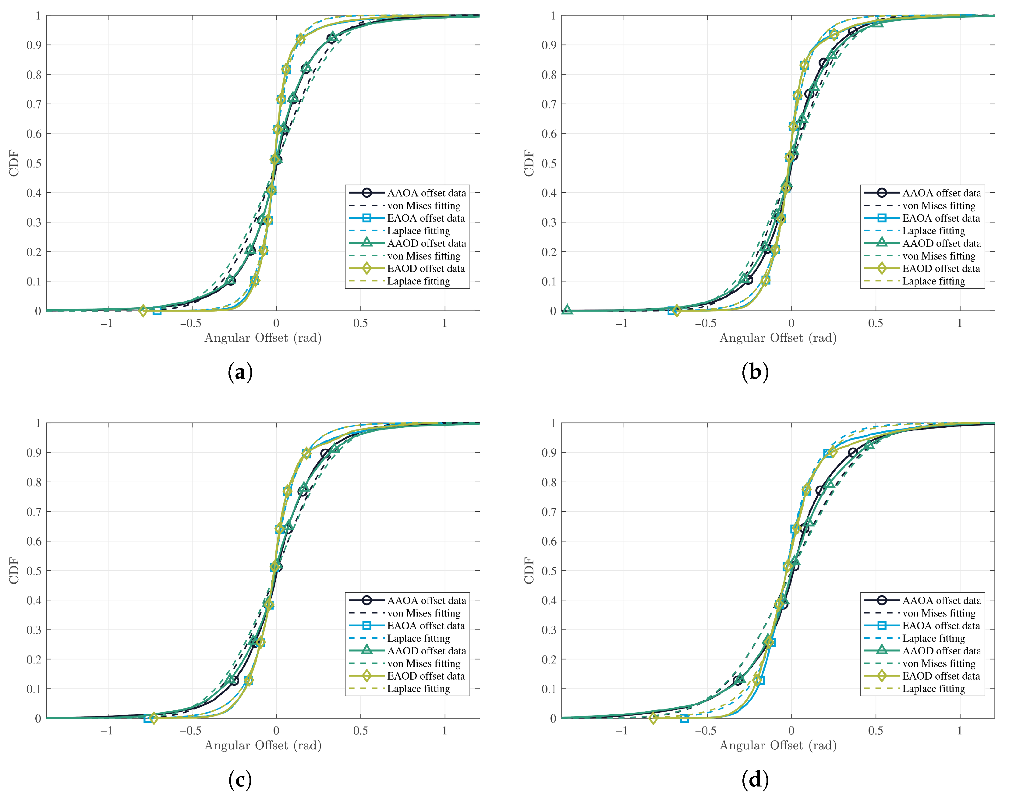
Figure 8 illustrates the CDF curves of angular offsets under different scenarios, along with their respective fitting results. In this study, the elevation angular offsets were fitted using the Laplace distribution, while the von Mises distribution was applied to the azimuth angular offsets. The corresponding fitting parameters are listed in Table 3. As shown in the figure, most angular offsets across scenarios are concentrated within the range of $[-1,1]$ radians, with azimuth offsets exhibiting a wider spread than elevation offsets, consistent with earlier statistical observations. Furthermore, the fitting parameters indicate that, as the urban environment becomes denser, the concentration parameter $\kappa$ of the von Mises distribution decreases, reflecting reduced concentration of azimuth offsets. In contrast, the scale parameter b of the Laplace distribution increases, suggesting a broader spread of elevation offsets. This trend can be attributed to the increased building heights and reduced inter-building spacing, which diversify signal propagation paths in both the horizontal and vertical directions, thereby expanding the range of intra-cluster azimuth and elevation angular offsets.

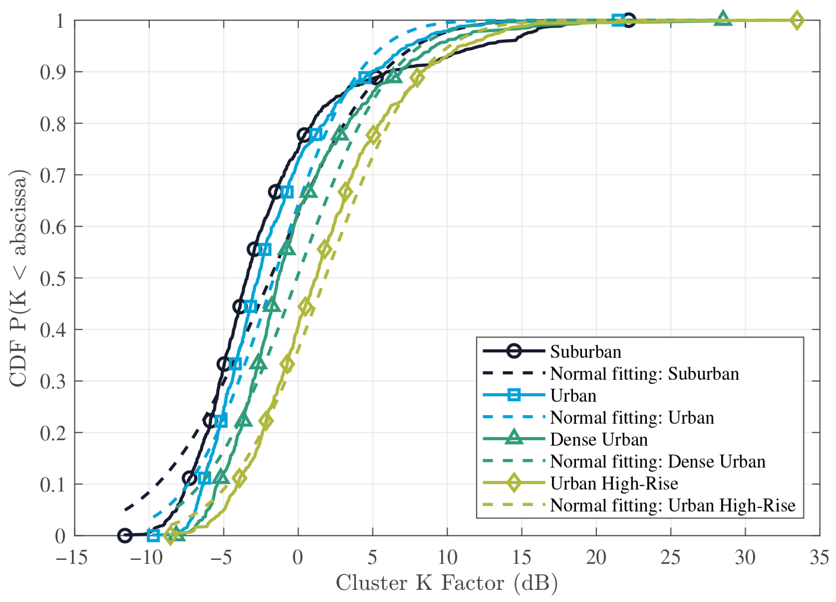
Figure 9 illustrates the CDFs of the cluster Rician K-factor across different scenarios. It is observed that the normal distribution provided a good fit for modeling the K-factor. The means of the fitted distributions from suburban to urban high-rise environments were −1.8687, −1.6384, −0.0867, and 1.8006 dB, respectively. This indicates a gradual increase in the relative power of the dominant path within each cluster compared to the remaining MPCs. This trend may be attributed to the stronger signal attenuation in high-rise urban environments, where MPCs experience more severe power decay due to the presence of tall buildings.

Figure 10 presents the spatial distribution of clusters at different Rx altitudes, with the CDF results for the urban high-rise scenario used as a representative example. Specifically, Figure 10a illustrates the distribution of azimuth angles, while Figure 10b depicts the distribution of elevation angles. The azimuth angles were mainly distributed between −3.1 and 3 radians, whereas the elevation angles ranged from 1.6 to 2.6 radians. In UAV A2A communication scenarios, scatterers are generally distributed in multiple directions on the horizontal plane, resulting in a wide range of azimuth angles. Further analysis shows that as the altitude of the Rx UAV decreased, the elevation angle exhibited a clear downward trend. This is because the height difference between building scatterers and the Rx decreased, leading to a narrower range of elevation angles. Consequently, the elevation angle distribution in UAV A2A scenarios became more concentrated, highlighting the unique characteristics of A2A channels.

Following the data acquisition method described in Section 2.1, 50 Txs were deployed at an altitude of 150 m and 400 Rxs at an altitude of 140 m. We obtained 20,000 unique UAV A2A channels by applying the RT method. Each Tx–Rx pair contained approximately 100 valid MPCs, thus forming a dataset with approximately 2,000,000 intra-cluster angular offset elements. These offset elements captured diverse spatial features and environmental propagation characteristics, providing a comprehensive statistical representation of intra-cluster multipath distributions in UAV A2A channels.

To adapt to the learning characteristics of periodic angular variables, angular offset data were first transformed onto a 2D Cartesian coordinate system using trigonometric encoding (i.e., cosine and sine components) prior to training the generative network. The generator took high-dimensional noise vectors sampled from a standard Gaussian distribution as input and consisted of multiple fully connected hidden layers. Each hidden layer was followed by batch normalization and a LeakyReLU activation function to enhance training stability and accelerate convergence. The final output was mapped to a 2D vector via a Tanh activation function, representing the cosine and sine components of the angular offset. The discriminator received a 2D input vector, either from real data or the generator’s output, and similarly employed a multi-layer fully connected architecture. LeakyReLU activation was used in the hidden layers, along with dropout and layer normalization techniques to prevent overfitting. The final output was a scalar representing the critic’s score of the input sample. During training, the generator and discriminator were updated using the RMSprop optimizer with an initial learning rate of $5\times {10}^{-5}$. A StepLR scheduler with a decay rate of $0.98$ every 500 steps was applied to improve training stability. The discriminator was updated five times per training iteration to maintain sufficient constraint over the generator. A gradient penalty term ($\lambda =5$) was introduced to enforce the Lipschitz continuity condition, thereby enabling effective optimization of the Wasserstein distance.

Based on the intra-cluster angular offset data from RT, we trained separate WGAN-GP networks for modeling elevation and azimuth angular offsets. Taking the high-rise urban scenario as an example, we selected the angle of arrival as a representative feature and compared the output of the generative model with the RT data and conventional statistical fitting methods. As shown in Figure 11, the results produced by the WGAN-GP model were more consistent with the RT data than those obtained by conventional statistical distributions. Unlike conventional methods that rely on predefined distribution forms, the generative approach flexibly learned the underlying relationships within the data, demonstrating superior adaptability and generalization capabilities. Furthermore, once trained, the generative model efficiently produced samples without repeated measurements or simulations, making it highly suitable for channel modeling across various scenarios.

Figure 12 illustrates the mean absolute percentage error between the generated data, conventional fitting methods, and the real data in terms of their PDFs across different scenarios. To mitigate error amplification in regions with low PDF values, the calculation was restricted to areas where the PDF exceeded 0.1. The results demonstrate that the generative approach consistently maintained an error below 10% in all scenarios, indicating superior fitting accuracy and robustness. In contrast, the conventional fitting methods exhibited larger and more variable errors, highlighting their limitations in capturing complex distribution characteristics and their relatively lower applicability.

In addition, the Kolmogorov–Smirnov and Cramer–von Mises statistics [40] were employed to quantitatively evaluate the agreement between the generated data, conventional fitted distributions, and the RT data. As shown in

Table 4. Comparison of the Kolmogorov–Smirnov and Cramer–von Mises statistics between fitted, generated, and RT data for azimuth angle offsets in the four urban scenarios.

Scenario	Kolmogorov–Smirnov		Cramer–von Mises
	Fit vs. RT	Generated vs. RT	Fit vs. RT	Generated vs. RT
Suburban	0.06709	0.02787	0.00165	0.00006
Urban	0.06292	0.03456	0.00123	0.00011
Dense urban	0.05592	0.02232	0.00118	0.00007
Urban high-rise	0.07588	0.02487	0.00230	0.00007

and

Table 5. Comparison of the Kolmogorov–Smirnov and Cramer–von Mises statistics between fitted, generated, and RT data for elevation angle offsets in the four urban scenarios.

Scenario	Kolmogorov–Smirnov		Cramer–von Mises
	Fit vs. RT	Generated vs. RT	Fit vs. RT	Generated vs. RT
Suburban	0.03299	0.03268	0.00031	0.00005
Urban	0.04447	0.03200	0.00045	0.00007
Dense urban	0.02605	0.01790	0.00033	0.00002
Urban high-rise	0.04179	0.01698	0.00065	0.00002

, the intra-cluster angular offsets generated by the proposed method exhibited lower Kolmogorov–Smirnov and Cramer–von Mises statistics across different scenarios compared to the fitted distributions, indicating a higher level of consistency with the RT data and further confirming the performance advantages of the generative approach.

5. Conclusions

This study investigated the clustering characteristics of UAV A2A channels in typical low-altitude urban scenarios. A set of 3D virtual scenarios was constructed, including suburban, urban, dense urban, and urban high-rise settings, and channel parameters were obtained through RT simulations. An automatic clustering method based on KPD was employed to group MPCs without the need to predefine the number of clusters. Based on the clustering results, a WGAN-GP model was introduced to learn and generate intra-cluster azimuth and elevation angular offsets. The results showed that as the scenario transitioned from suburban to urban high-rise, the number of MPCs per cluster decreased, while the intra-cluster delay and elevation angular spreads increased. Azimuth angles were broadly distributed, whereas elevation angles tended to concentrate due to the spatial distribution of scatterers. Compared to conventional empirical distributions such as Laplacian and von Mises, the proposed generative model produced angular offset data that were more consistent with the RT data. Overall, the proposed framework provides an effective approach for analyzing cluster characteristics in UAV A2A channels and demonstrates strong adaptability across different propagation scenarios. In future work, we will further study cluster characteristics under more complex scenarios using advanced deep learning techniques.

References

1. Hua, B.; Han, L.; Zhu, Q.; Wang, C.X.; Mao, K.; Bao, J.; Chang, H.; Tang, Z. Ultra-Wideband Nonstationary Channel Modeling for UAV-to-Ground Communications. IEEE Trans. Wirel. Commun. 2025, 24, 4190–4204. [Google Scholar] [CrossRef]
2. Jiang, H.; Shi, W.; Zhang, Z.; Pan, C.; Wu, Q.; Shu, F.; Liu, R.; Chen, Z.; Wang, J. Large-Scale RIS Enabled Air-Ground Channels: Near-Field Modeling and Analysis. IEEE Trans. Wirel. Commun. 2025, 24, 1074–1088. [Google Scholar] [CrossRef]
3. Wang, J.; Zhu, Q.; Lin, Z.; Chen, J.; Ding, G.; Wu, Q.; Gu, G.; Gao, Q. Sparse Bayesian Learning-Based Hierarchical Construction for 3D Radio Environment Maps Incorporating Channel Shadowing. IEEE Trans. Wirel. Commun. 2024, 23, 14560–14574. [Google Scholar] [CrossRef]
4. Lian, Z.; Zhang, W.; Wang, Y.; Su, Y.; Zhang, B.; Jin, B.; Wang, B. Physics-Based Channel Modeling for IRS-Assisted mmWave Communication Systems. IEEE Trans. Commun. 2024, 72, 2687–2700. [Google Scholar] [CrossRef]
5. Ede, B.; Kaplan, B.; Kahraman, İ.; Keşir, S.; Yarkan, S.; Ekti, A.R.; Baykaş, T.; Görçin, A.; Çırpan, H.A. Measurement-Based Large Scale Statistical Modeling of Air–to–Air Wireless UAV Channels via Novel Time–Frequency Analysis. IEEE Wirel. Commun. Lett. 2022, 11, 136–140. [Google Scholar] [CrossRef]
6. Guo, L.; Guan, K.; Liu, T.; He, D.; Zhang, H.; Zhu, Q.; Lu, J.; Zhang, M. Obtaining electromagnetic properties of multi-type media in realistic environments: State-of-the-art and prospects. China Commun. 2025, 22, 25–40. [Google Scholar] [CrossRef]
7. Zhu, G.; Liu, Y.; Li, S.; Mao, K.; Zhu, Q.; Briso-Rodríguez, C.; Liang, J.; Ye, X. Semantic-Based Channel State Information Feedback for AAV-Assisted ISAC Systems. IEEE Internet Things J. 2025, 12, 4981–4991. [Google Scholar] [CrossRef]
8. Liu, X.; Zhong, W.; Wang, X.; Duan, H.; Fan, Z.; Jin, H.; Huang, Y.; Lin, Z. Deep Reinforcement Learning-Based 3D Trajectory Planning for Cellular Connected UAV. Drones 2024, 8, 199. [Google Scholar] [CrossRef]
9. Molisch, A.; Tufvesson, F. Propagation Channel Models for Next-Generation Wireless Communications Systems. IEICE Trans. Commun. 2014, 97, 2022–2034. [Google Scholar] [CrossRef]
10. Zeng, L.; Liao, X.; Ma, Z.; Liu, W.; Jiang, H.; Chen, Z. Toward More Adaptive UAV-to-UAV GBSMs: Introducing the Extended vMF Distribution. IEEE Wirel. Commun. Lett. 2025, 14, 260–264. [Google Scholar] [CrossRef]
11. Chen, Z.; Guo, Y.; Zhang, P.; Jiang, H.; Xiao, Y.; Huang, L. Physical Layer Security Improvement for Hybrid RIS-Assisted MIMO Communications. IEEE Commun. Lett. 2024, 28, 2493–2497. [Google Scholar] [CrossRef]
12. Lee, J. Cluster-Based Millimeter-Wave Outdoor-to-Indoor Propagation Characteristics Based on 32 GHz Measurement Analysis. IEEE Antennas Wirel. Propag. Lett. 2021, 20, 73–77. [Google Scholar] [CrossRef]
13. Liu, L.; Oestges, C.; Poutanen, J.; Haneda, K.; Vainikainen, P.; Quitin, F.; Tufvesson, F.; Doncker, P.D. The COST 2100 MIMO channel model. IEEE Wirel. Commun. 2012, 19, 92–99. [Google Scholar] [CrossRef]
14. 3GPP. Enhanced LTE Support for Aerial Vehicles; Technical Report TR 36.777; Sophia Antipolis, France. 2018. Available online: https://www.3gpp.org/dynareport/36777.htm (accessed on 1 June 2025).
15. Bai, L.; Huang, Z.; Cheng, X. A non-stationary model with time-space consistency for 6G massive MIMO mmWave UAV channels. IEEE Trans. Wirel. Commun. 2022, 22, 2048–2064. [Google Scholar] [CrossRef]
16. Ge, C.; Zhang, R.; Jiang, Y.; Li, B.; He, Y. A 3-D Dynamic Non-WSS Cluster Geometrical-Based Stochastic Model for UAV MIMO Channels. IEEE Trans. Veh. Technol. 2022, 71, 6884–6899. [Google Scholar] [CrossRef]
17. Zhang, X.; Liu, J.; Gu, F.; Ma, D.; Wei, J. An extended 3-D ellipsoid model for characterization of UAV air-to-air channel. In Proceedings of the ICC 2019—2019 IEEE International Conference on Communications (ICC), Shanghai, China, 20–24 May 2019; pp. 1–6. [Google Scholar]
18. Ma, Z.; Ai, B.; He, R.; Zhong, Z.; Yang, M. A non-stationary geometry-based MIMO channel model for millimeter-wave UAV networks. IEEE J. Sel. Areas Commun. 2021, 39, 2960–2974. [Google Scholar] [CrossRef]
19. Zhang, K.; Wang, H.; Zhang, C.; Yu, X.; Dong, Y. Three-dimensional geometry-based stochastic model for sub-terahertz air-to-air UAV-MIMO channels. In Proceedings of the 2023 IEEE/CIC International Conference on Communications in China (ICCC), Dalian, China, 10–12 August 2023; pp. 1–6. [Google Scholar]
20. Hua, B.; Deng, Q.; Zhu, Q.; Wang, C.X.; Han, L.; Briso-Rodríguez, C.; Tang, Z.; Mao, K. A Novel A2A Channel Model Incorporating Rooftop Specular Reflection and Airframe Occlusion. IEEE Trans. Wirel. Commun. 2025. [Google Scholar] [CrossRef]
21. Hua, B.; Han, L.; Deng, Q.; Zhu, Q.; Li, H.; Qu, Y.; Briso-Rodríguez, C.; Mao, K. AAV Air-to-Air Channel: Statistical Properties and Experimental Verification. IEEE Internet Things J. 2025, 12, 25790–25803. [Google Scholar] [CrossRef]
22. Huang, C.; He, R.; Ai, B.; Molisch, A.F.; Lau, B.K.; Haneda, K.; Liu, B.; Wang, C.X.; Yang, M.; Oestges, C.; et al. Artificial Intelligence Enabled Radio Propagation for Communications—Part I: Channel Characterization and Antenna-Channel Optimization. IEEE Trans. Antennas Propag. 2022, 70, 3939–3954. [Google Scholar] [CrossRef]
23. Ma, Z.; Zhang, R.; Ai, B.; Lian, Z.; Zeng, L.; Niyato, D.; Peng, Y. Deep Reinforcement Learning for Energy Efficiency Maximization in RSMA-IRS-Assisted ISAC System. IEEE Trans. Veh. Technol. 2025, 1–6. [Google Scholar] [CrossRef]
24. Luo, J.; Liao, X.; Wang, Y.; Zhang, J.; Yu, Z.; Wang, G.; Li, X. An Entropy-Based Adaptive DBSCAN Clustering Algorithm and Its Application in THz Wireless Channels. IEEE Trans. Antennas Propag. 2023, 71, 9830–9837. [Google Scholar] [CrossRef]
25. Huang, Z.; Zhang, R.; Pan, J.; Jiang, Y.; Zhai, D. A Framework of Multipath Clustering Based on Space-Transformed Fuzzy c-Means and Data Fusion for Radio Channel Modeling. IEEE Trans. Veh. Technol. 2020, 69, 4–15. [Google Scholar] [CrossRef]
26. Zhou, T.; Qiao, Y.; Salous, S.; Liu, L.; Tao, C. Machine Learning-Based Multipath Components Clustering and Cluster Characteristics Analysis in High-Speed Railway Scenarios. IEEE Trans. Antennas Propag. 2022, 70, 4027–4039. [Google Scholar] [CrossRef]
27. Zhang, Z.; Liu, Y.; Wang, C.X.; Chang, H.; Bian, J.; Zhang, J. Machine Learning Based Clustering and Modeling for 6G UAV-to-Ground Communication Channels. IEEE Trans. Veh. Technol. 2024, 73, 14113–14126. [Google Scholar] [CrossRef]
28. Cui, Z.; Guan, K.; Oestges, C.; Briso-Rodríguez, C.; Ai, B.; Zhong, Z. Cluster-Based Characterization and Modeling for UAV Air-to-Ground Time-Varying Channels. IEEE Trans. Veh. Technol. 2022, 71, 6872–6883. [Google Scholar] [CrossRef]
29. Lyu, Y.; Xue, B.; Wang, W. A Genetic Algorithm-Based Iterative Channel Estimation Method for Ranging Applications in Closely Spaced Multipath Environment. IEEE Antennas Wirel. Propag. Lett. 2025, 24, 1327–1331. [Google Scholar] [CrossRef]
30. Lyu, Y.; Wang, W.; Chen, P. Fixed-Wing UAV-Based Air-to-Ground Channel Measurement and Modeling at 2.7 GHz in a Rural Environment. IEEE Trans. Antennas Propag. 2025, 73, 2038–2052. [Google Scholar] [CrossRef]
31. ITU-R. Propagation Data and Prediction Methods for the Design of Terrestrial Broadband Millimetric Radio Access Systems; Recommendation ITU-R P.1410-2; International Telecommunication Union: Geneva, Switzerland, 2003; Available online: https://www.itu.int/rec/R-REC-P.1410/en (accessed on 1 June 2025).
32. Du, F.; Zhao, X.; Zhang, Y.; Wen, Y.; Fu, Z.; Geng, S.; Qin, P.; Zhou, Z.; Xu, C.; Liu, Y.; et al. SVM-Assisted Adaptive Kernel Power Density Clustering Algorithm for Millimeter Wave Channels. IEEE Trans. Antennas Propag. 2022, 70, 4014–4026. [Google Scholar] [CrossRef]
33. Czink, N.; Cera, P.; Salo, J.; Bonek, E.; Nuutinen, J.P.; Ylitalo, J. Improving clustering performance using multipath component distance. Electron. Lett. 2006, 42, 33–35. [Google Scholar] [CrossRef]
34. He, R.; Li, Q.; Ai, B.; Geng, Y.L.A.; Molisch, A.F.; Kristem, V.; Zhong, Z.; Yu, J. A Kernel-Power-Density-Based Algorithm for Channel Multipath Components Clustering. IEEE Trans. Wirel. Commun. 2017, 16, 7138–7151. [Google Scholar] [CrossRef]
35. Rousseeuw, P.J. Silhouettes: A graphical aid to the interpretation and validation of cluster analysis. J. Comput. Appl. Math. 1987, 20, 53–65. [Google Scholar] [CrossRef]
36. Meinilä, J.; Kyösti, P.; Hentilä, L.; Jämsä, T.; Suikkanen, E.; Kunnari, E.; Narandžić, M. Document Title: D5. 3: WINNER+ Final Channel Models 2010. Available online: https://www.researchgate.net/publication/261467821 (accessed on 1 June 2025).
37. Mao, K.; Zhu, Q.; Wang, C.X.; Ye, X.; Gomez-Ponce, J.; Cai, X.; Miao, Y.; Cui, Z.; Wu, Q.; Fan, W. A Survey on Channel Sounding Technologies and Measurements for UAV-Assisted Communications. IEEE Trans. Instrum. Meas. 2024, 73, 1–24. [Google Scholar] [CrossRef]
38. Arjovsky, M.; Chintala, S.; Bottou, L. Wasserstein generative adversarial networks. In Proceedings of the International Conference on Machine Learning, PMLR, Sydney, Australia, 6–11 August 2017; pp. 214–223. [Google Scholar]
39. Gulrajani, I.; Ahmed, F.; Arjovsky, M.; Dumoulin, V.; Courville, A.C. Improved training of wasserstein GANs. In Proceedings of the Advances in Neural Information Processing Systems, Red Hook, NY, USA, 4–9 December 2017; pp. 5769–5779. [Google Scholar]
40. Ziółkowski, C.; Kelner, J.M. Empirical models of the azimuthal reception angle—Part I: Comparative analysis of empirical models for different propagation environments. Wirel. Pers. Commun. 2016, 91, 771–791. [Google Scholar] [CrossRef]
Figure 1. Illustration of the channel model for A2A communication.
Drones 09 00586 g001
Figure 2. Reconstructed typical urban scenarios: (a) suburban; (b) urban; (c) dense urban; (d) urban high-rise.
Drones 09 00586 g002
Figure 3. 3D visualization of clustering results in (a) suburban; (b) urban; (c) dense urban; (d) urban high-rise areas.
Drones 09 00586 g003
Figure 4. The network structure of the WGAN-GP.
Drones 09 00586 g004
Figure 5. The CDFs of the number of MPCs per cluster: (a) suburban; (b) urban; (c) dense urban; (d) urban high-rise.
Drones 09 00586 g005
Figure 6. The CDFs of cluster RMS-DSs for different scenarios.
Drones 09 00586 g006
Figure 7. The CDFs of cluster RMS-ASs for different scenarios: (a) suburban; (b) urban; (c) dense urban; (d) urban high-rise.
Drones 09 00586 g007
Figure 8. The CDFs of angular offsets for different scenarios: (a) suburban; (b) urban; (c) dense urban; (d) urban high-rise.
Drones 09 00586 g008
Figure 9. The CDFs of cluster Rician K-factor for different scenarios.
Drones 09 00586 g009
Figure 10. Cluster space distributions for different altitudes of (a) azimuth and (b) elevation.
Drones 09 00586 g010
Figure 11. PDFs of training data, generated angle offsets, and conventional methods of (a) elevation and (b) azimuth.
Drones 09 00586 g011
Figure 12. The space distribution of cluster locations.
Drones 09 00586 g012