Path Planning for Unmanned Aerial Vehicle: A-Star-Guided Potential Field Method ^†

Abstract

The utilization of Unmanned Aerial Vehicles (UAVs) in missions such as reconnaissance and surveillance has grown rapidly, underscoring the need for efficient path planning algorithms that ensure both optimality and collision avoidance. The A-star algorithm is widely used for global path planning due to its ability to generate optimal routes; however, its high computational cost makes it unsuitable for real-time applications, particularly in unknown or dynamic environments. For local path planning, the Artificial Potential Field (APF) algorithm enables real-time navigation by attracting the UAV toward the target while repelling it from obstacles. Despite its efficiency, APF suffers from local minima and limited performance in dynamic settings. To address these challenges, this paper proposes the A-star-Guided Potential Field (AGPF) algorithm, which integrates the strengths of A-star and APF to achieve robust performance in both global and local path planning. The AGPF algorithm was validated through simulations conducted in the Robot Operating System (ROS) environment. Simulation results demonstrate that AGPF produces smoother and more optimal paths than A-star, while avoiding the local minima issues inherent in APF. Furthermore, AGPF effectively handles moving and previously unknown obstacles by generating real-time avoidance trajectories, demonstrating strong adaptability in dynamic and uncertain environments.

1. Introduction

In recent years, Unmanned Aerial Vehicles (UAVs) have seen a significant rise in use across the defense and commercial sectors due to their cost efficiency and ability to access hazardous or hard-to-reach areas [1,2,3,4]. This growing demand is particularly evident in military operations, disaster management, and emergency response, where UAVs are utilized for tasks such as reconnaissance, surveillance, and search-and-rescue missions. For example, UAVs played a pivotal role in wars, being recognized as game-changers that can influence the outcome of conflicts [5]. In rescue missions, UAVs not only indirectly support rescue operations, such as finding victims [6], but they are also used to perform rescue operations directly, such as delivering flotation devices to victims [7]. In architectural engineering, construction management, and monitoring, a fully automated intelligent construction monitoring and reporting system is also being developed based on real-time data obtained from UAVs [8]. To effectively complete these missions, the path planning algorithm is a core module of the UAV’s flight software. The algorithm should create a safe and cost-effective path for the given mission.

The path planning algorithm can be categorized into global path planning or local path planning, as shown in Figure 1. The global path is primarily built with static environmental data, such as maps or point cloud datasets [9]. The global path algorithm mainly focuses on creating a stable and optimal path to complete missions. A-star [10,11,12,13], one of the most common global path planning algorithms, is a graph-based algorithm that calculates an optimal path using static environmental data. A limitation of A-star is that it is hard to work in dynamic or unknown environments because it needs to regenerate a path whenever it is updated. To alleviate the limitation, several enhanced algorithms, such as D-star [14,15], LPA-star [16], and D-star lite [17], have been proposed. These algorithms efficiently handle environmental changes by recalculating only the essential part of the environment to capture the variation. Guan [18] and Liao [19] combined A-star with the Dynamic Window Approach (DWA), which calculates avoidance paths based on the speed, direction, and distance of dynamic obstacles. He [20] proposed a Dynamic Anti-collision A-star algorithm, which integrates time factors to improve dynamic obstacle avoidance. Another limitation of the A-star algorithm is that it builds an unsmooth path, including sharp turns and discontinuous segments. It is challenging for vehicles to trace the path due to the restriction of their turning performance. To mitigate the limitation, various concepts have been employed to generate a smooth path for vehicles. For example, theta-star [21] utilizes line-of-sight to reduce the connectivity of intermediate nodes, making the path as straight as possible to generate a smoother path. Liu [22] used the Bezier curve method to transform the unsmooth segments of the A-star path into a smooth curved path.

On the other hand, the local path algorithm generates flight paths by utilizing real-time environmental information collected from various sensors such as cameras [23] or LiDAR [24], which focuses on effectively avoiding unknown or dynamic obstacles that the global path cannot account for. Moreover, the algorithm needs to consider how the vehicle returns smoothly to the global path after avoiding obstacles [25]. The Artificial Potential Field (APF) method [26,27,28,29] is widely used in local path planning due to its simplicity and intuitive design, employing attractive forces toward the goal and repulsive forces away from obstacles. However, APF suffers from limitations such as susceptibility to local minima and reduced effectiveness in environments with dynamic obstacles. To alleviate limitations, Du [25], Qixin [30], and Ge [31] proposed the Dynamic Artificial Potential Field (DAPF), which applies a new repulsive force that considers the relative velocity of dynamic obstacles to generate avoidance paths. Meanwhile, several improved APF algorithms have been proposed to relieve the local minima issue. Sheng [32] developed an enhanced APF that generates virtual target points to help escape local minima. Li [33] handled the local minima issue by altering the direction of the repulsive force acting on the vehicle.

In addition, since the APF method relies on a simple resultant force calculation, it lacks a systematic framework to ensure path optimality and cannot guarantee the derivation of an optimal route. To overcome this limitation, Ju [34] proposed a hybrid algorithm that combines the optimal pathfinding capabilities of the A-star algorithm with the smooth trajectory generation of the APF method. This fusion approach mitigates the respective weaknesses of both techniques by refining the coarse paths generated by A-star and enhancing the APF’s ability to produce smoother and more optimal trajectories. However, the proposed method primarily operates under the assumption of a static environment and remains vulnerable to local minima in certain configurations. As a result, its applicability is limited in real-world scenarios, where dynamic environmental changes occur during operation and continuous adaptability is required.

Recently, hybrid path planning strategies that combine the complementary strengths of multiple algorithms at both global and local levels have attracted considerable attention for their ability to enhance robustness and adaptability in dynamic environments. For example, Liu [35] proposed the G-APF algorithm, which integrates the Artificial Potential Field (APF) framework into the Rapidly exploring Random Tree (RRT) structure, enabling the simultaneous generation of feasible global and local paths. Similarly, Xu [36] introduced a two-layer planning scheme that combines bidirectional A-star for global path generation with the Dynamic Window Approach (DWA) for local navigation, guided by key waypoints extracted from the global path. These hybrid approaches have demonstrated improved real-time adaptability and obstacle avoidance in complex and changing environments.

Building upon these prior studies, this paper proposes the A-star-Guided Potential Field (AGPF) algorithm, which extends Ju’s fusion approach by enhancing adaptability to dynamic environments and improving local obstacle avoidance capabilities. The core idea of the AGPF algorithm was preliminarily explored in our earlier work [37], and this study further develops and formalizes the method with enhanced structure and performance analysis. The proposed method comprises two primary components: global and local path planning. The global path planning module generates a smooth and near-optimal trajectory toward the target by leveraging Ju’s fusion method. To address the local minima problem often associated with hybrid potential field approaches, a complementary technique is introduced. The local path planning module implements a real-time reactive strategy that enables the vehicle to avoid collisions with previously unknown or dynamic obstacles. Additionally, a recovery strategy is integrated to guide the vehicle back to the globally planned path following an avoidance maneuver.

The remainder of this paper is organized as follows. Section 2 reviews the conventional A-star and APF algorithms. Section 3 describes the proposed AGPF-based global and local path planning approach. Section 4 demonstrates the proposed AGPF algorithm with several scenarios in the Robot Operating System (ROS) environment. Finally, Section 5 provides concluding remarks.

2. Traditional Path Planning Algorithm

2.1. A-Star Algorithm

The A-star algorithm is one of the most widely used graph search algorithms with static environment information. It represents the environment as a grid map, where each grid’s center point serves as a node. The algorithm constructs an optimal path by properly connecting appropriate nodes unless obstacles surround the vehicle. The A-star algorithm is developed by incorporating heuristic methods into the Dijkstra algorithm, and it uses the following heuristic objective function, where

$$f\left(n\right)=g\left(n\right)+h\left(n\right)$$

(1)

where n is the current inspection node; $g\left(n\right)$ is the actual cost of the path from the start node to the current node; $h\left(n\right)$ is the estimated cost calculated by Euclidean distance from the current node n to the target node such that

$$h\left(n\right)=\sqrt{{(x_n-x_{\mathrm{g}})}^2+{(y_n-y_{\mathrm{g}})}^2}$$

(2)

where $(x_n,y_n)$, $(x_{\mathrm{g}},y_{\mathrm{g}})$ are the coordinates of the inspection node and the target node, respectively.

A well-known disadvantage of the A-star algorithm is that it creates piecewise linear paths, including sharp turns. To alleviate the limitation, decreasing the grid size would be beneficial, but it significantly increases the problem size to solve. Moreover, to reflect the changes in the surrounding environmental information, all grid states should be reset, and then the path is updated. Due to these restrictions, A-star is mostly used for global path planning rather than real-time local path planning.

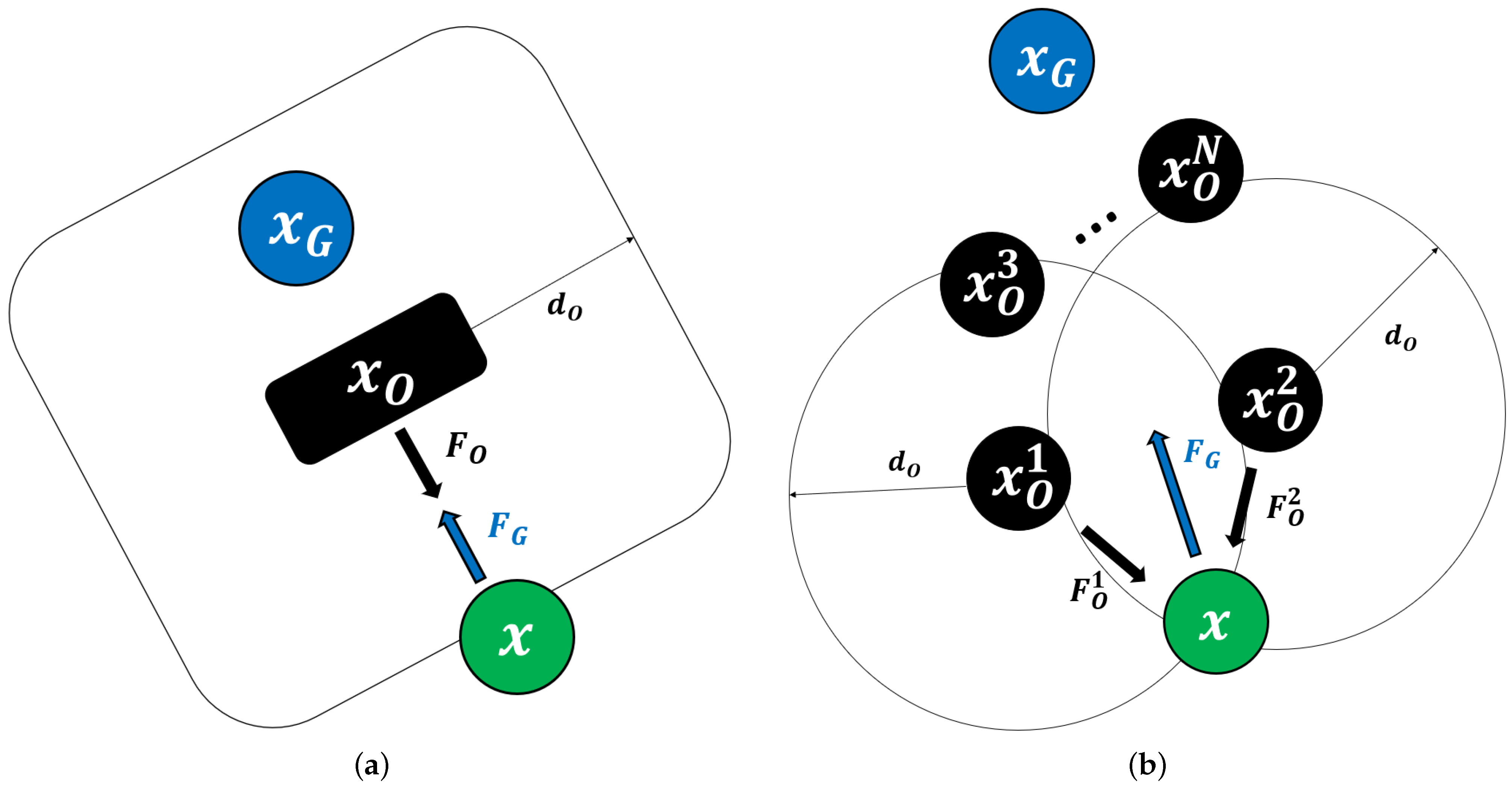
2.2. Artificial Potential Field Algorithm

Artificial Potential Field (APF) is an algorithm that produces a path from the start point to the target based on virtual potential fields to avoid obstacles. It employs two potential fields: a virtual attractive field and a virtual repulsive field. While the virtual attractive field pulls the vehicle toward the target, guiding it to the target, the virtual repulsive field pushes the vehicle away from obstacles, enabling it to avoid collisions. The attractive and repulsive fields at a specific position $\mathit{x}$ are

$$\begin{array}{cc}\hfill U_G\left({\mathit{\rho }}_G\right)& ={\displaystyle \frac{1}{2}}{K}_G{\parallel {\mathit{\rho }}_G\parallel }^2\hfill \end{array}$$

(3)

$$\begin{array}{cc}\hfill U_O\left({\mathit{\rho }}_O\right)& =\left\{\begin{array}{cc}{\displaystyle \frac{1}{2}}{K}_O{e}^{-l_O{\parallel {\mathit{\rho }}_O\parallel }^2}\hfill & \mathrm{if}\parallel {\mathit{\rho }}_O\parallel \le d_O\hfill \\ 0\hfill & \mathrm{if}\parallel {\mathit{\rho }}_O\parallel >d_O\hfill \end{array}\right.\hfill \end{array}$$

(4)

$$\begin{array}{cc}\hfill with{\mathit{\rho }}_G& ={\mathit{x}}_G-\mathit{x},{\mathit{\rho }}_O={\mathit{x}}_O-\mathit{x}\hfill \end{array}$$

where $K_G$, $K_O$ are the attractive field and repulsive field coefficients, respectively; ${\mathit{x}}_G$ is the position of the target; ${\mathit{x}}_O$ is the position of the obstacle; $d_O$ is a distance threshold that the repulsive force begins to exert; $l_O$ is the coefficient that changes the form of the repulsive force.

The total potential field is formed by the superposition of attractive and repulsive components, which together define the configuration space and guide the vehicle’s trajectory. The path is generated by following the direction of decreasing potential, determined by the potential difference between the current position and its surroundings. This process can be interpreted as the vehicle descending along the gradient of the potential field toward a local minimum. To facilitate this behavior, the gradient at the current position is computed, representing both the direction and magnitude of the virtual force acting on the vehicle. Accordingly, the attractive force and repulsive force at $\mathit{x}$ are calculated by the negative gradient of Equations (3) and (4), where

$$\begin{array}{cc}\hfill {\mathbf{F}}_G& =-\nabla U_G\left({\mathit{\rho }}_G\right)=-{\displaystyle \frac{\partial U_G\left({\mathit{\rho }}_G\right)}{\partial \mathit{x}}}=K_G{\mathit{\rho }}_G\hfill \end{array}$$

(5)

$$\begin{array}{cc}\hfill {\mathbf{F}}_O& =-\nabla U_O\left({\mathit{\rho }}_O\right)=-{\displaystyle \frac{\partial U_O\left({\mathit{\rho }}_O\right)}{\partial \mathit{x}}}=\left\{\begin{array}{cc}{K}_O{l}_O{\mathit{\rho }}_O{e}^{-l_o{\parallel {\mathit{\rho }}_O\parallel }^2}\hfill & \mathrm{if}\parallel {\mathit{\rho }}_O\parallel \le d_O\hfill \\ 0\hfill & \mathrm{if}\parallel {\mathit{\rho }}_O\parallel >d_O\hfill \end{array}\right.\hfill \end{array}$$

(6)

where ${\mathit{F}}_G$ and ${\mathit{F}}_O$ are the attractive and repulsive force, respectively. The attractive force is proportional to the distance between the target and $\mathit{x}$. The magnitude of the attractive force is determined by the coefficient $K_G$.

The change in the repulsive force according to the $\parallel {\mathit{\rho }}_O\parallel$ is shown in Figure 2. Based on A, the relationship between the repulsive force and $\parallel {\mathit{\rho }}_O\parallel$ exhibits two tendencies, such that if the repulsive force is less than A, it increases as $\parallel {\mathit{\rho }}_O\parallel$ increases, whereas if the repulsive force is greater than A, it decreases as $\parallel {\mathit{\rho }}_O\parallel$ increases. When considering the physical relationship between obstacle avoidance and the repulsive force, the maximum repulsive force, B, should be sufficiently large to push the vehicle away from obstacles, and $d_O$ needs to be greater than A. Because the values of A and B are based on the coefficients $K_O$ and $l_O$, the coefficients $K_O$ and $l_O$ should be appropriately adjusted to build a collision-free path.

Using ${\mathit{F}}_G$ and ${\mathit{F}}_O$, the total force at $\mathit{x}$ can be represented as shown in Figure 3 and defined by Equation (7), where

$${\mathit{F}}_{Tot}={\mathit{F}}_{Att}+{\mathit{F}}_{Rep}={\mathit{F}}_G+\sum _{i=1}^N{\mathit{F}}_O^i$$

(7)

where ${\mathit{F}}_{Tot}$ is the total force, representing the direction from $\mathit{x}$ to the next point; ${\mathit{F}}_{Att}$ is the sum of attractive force, which is equal ${\mathit{F}}_G$; ${\mathit{F}}_{Rep}$ is the sum of repulsive forces from N obstacles; ${\mathit{F}}_O^i$ is the $i_{th}$ obstacle’s repulsive force.

In the traditional APF, when the total force acting at the $\mathit{x}$ becomes zero, the method cannot determine a direction to move, which means the path terminates at the $\mathit{x}$ called a local minimum problem. As shown in Figure 4, a local minimum situation in APF occurs in two cases.

Figure 4a represents a case where the target, an obstacle, and the vehicle at $\mathit{x}$ are aligned in a straight line. In this case, the obstacle entirely blocks the attractive force, making it impossible to form a path to the target. Figure 4b illustrates that although the obstacles do not entirely block the attractive force, the repulsive forces counteract it, resulting in a zero net force and ultimately preventing path formation. In both cases, the attractive and repulsive forces balance each other, trapping the vehicle at a local minimum.

As mentioned above, the APF algorithm has advantages such as being intuitive, easy to implement due to its simple structure, and having low computational complexity. However, if the APF-based system becomes trapped in local minima, it fails to generate a path to the target. Moreover, APF does not ensure the generation of an optimal path to the target and has limitations in creating avoidance paths for dynamic obstacles. Therefore, supplementary solutions that address these shortcomings are essential to apply the APF effectively in real-world path planning.

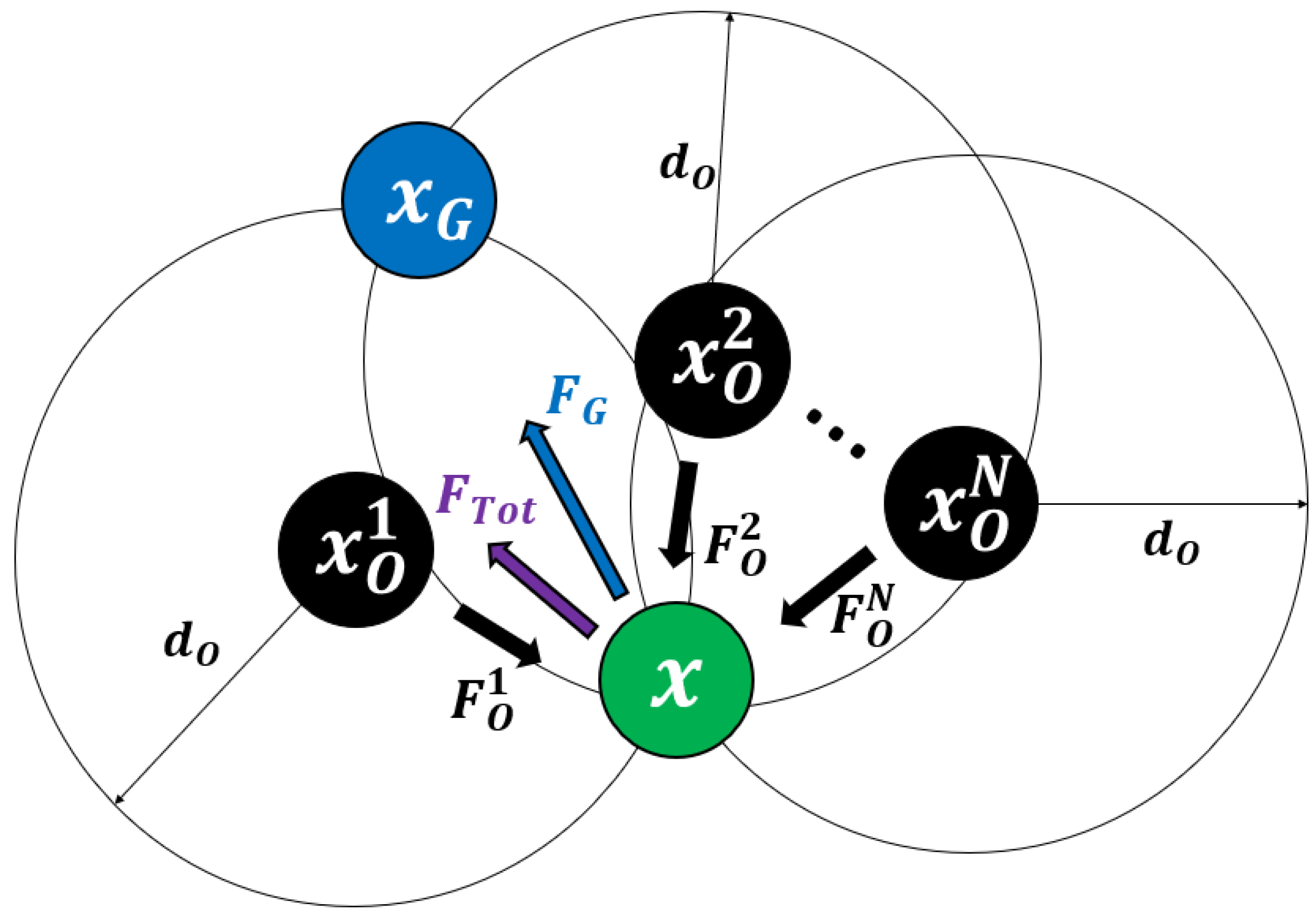
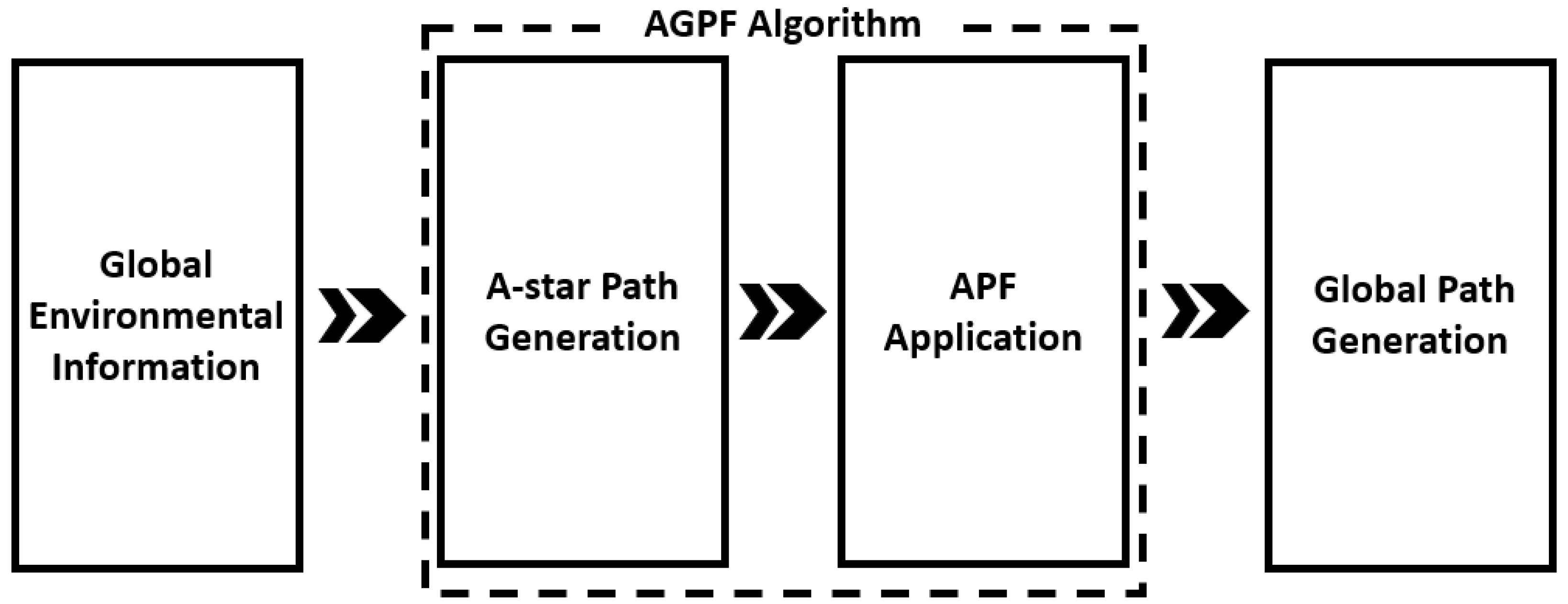
3. A-Star-Guided Potential Field Algorithm

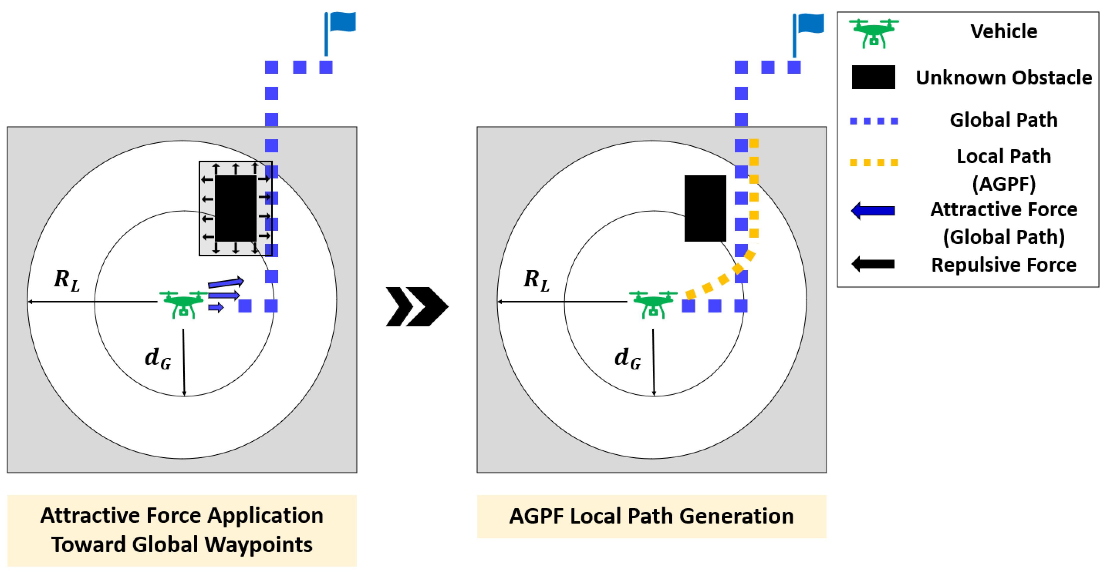
3.1. AGPF for Global Path Planning

The AGPF algorithm for global path planning consists of four modules: Global Environmental Information, A-star Path Generation, APF Application, and Global Path Generation, as shown in Figure 5.

In the Global Environmental Information step, environmental data relevant to the mission area is acquired to generate the global path planning. In this study, approximate environmental information about the mission area is assumed to be provided in advance. This information is the foundation for subsequent path generation and obstacle avoidance processes.

Next, in the A-star Path Generation step, the A-star algorithm utilizes the acquired environmental information to calculate an initial path from the start to the target. This path represents an optimal route based on the known environmental constraints. The generated waypoints are then transferred to the subsequent APF Application step.

In the APF Application step, the APF method is utilized to refine the path using stored A-star waypoints. Like the APF, the AGPF method generates a path utilizing virtual attractive and repulsive fields. However, unlike the traditional method that applies an attractive field directly to the target, the AGPF applies an attractive field to the waypoints generated by A-star instead. The attractive field at $\mathit{x}$ toward the A-star waypoint is

$$U_A\left({\mathit{\rho }}_A\right)=\left\{\begin{array}{cc}{\displaystyle \frac{1}{2}}{K}_A{\parallel {\mathit{\rho }}_A\parallel }^2\hfill & \mathrm{if}\parallel {\mathit{\rho }}_A\parallel \le d_A\hfill \\ 0\hfill & \mathrm{if}\parallel {\mathit{\rho }}_A\parallel >d_A\hfill \end{array}\right.$$

(8)

$$\begin{array}{cc}\hfill with{\mathit{\rho }}_A& ={\mathit{x}}_A-\mathit{x}\hfill \end{array}$$

where $K_A$ is the A-star attractive field coefficient; ${\mathit{x}}_A$ is the position of the A-star waypoint; $d_A$ is the distance at which the attraction toward the waypoint begins. The attractive force toward the A-star waypoint is calculated by the negative gradient of Equation (8), where

$${\mathrm{F}}_A=-\nabla U_A\left({\mathit{\rho }}_A\right)=-{\displaystyle \frac{\partial U_A\left({\mathit{\rho }}_A\right)}{\partial \mathit{x}}}=\{\begin{array}{cc}{K}_A{\mathit{\rho }}_A& \mathrm{if}\parallel {\mathit{\rho }}_A\parallel \le d_A\\ 0& \mathrm{if}\parallel {\mathit{\rho }}_A\parallel >d_A\end{array}$$

(9)

In contrast to the conventional APF algorithm that pulls the vehicle directly toward a fixed target position, the AGPF algorithm applies attractive forces toward multiple A-star waypoints within a specified distance $d_A$ from the vehicle’s current position $\mathit{x}$. For instance, the total force at $\mathit{x}$ is shown in Figure 6 and Equation (10).

$${\mathit{F}}_{Tot}={\mathit{F}}_{Att}+{\mathit{F}}_{Rep}=\sum _{j=1}^M{\mathit{F}}_A^j+\sum _{i=1}^N{\mathit{F}}_O^i$$

(10)

where ${\mathit{F}}_{Att}$ is the sum of attractive forces toward M A-star waypoints; ${\mathit{F}}_A^j$ is the $j_{th}$ A-star waypoint’s attractive force. In the traditional APF, the attractive force is directed solely toward the target rather than toward obstacle avoidance. When the target, an obstacle, and $\mathit{x}$ are aligned, the obstacle blocks the vehicle’s path to the target, causing it to become trapped in a local minimum. On the other hand, the AGPF algorithm applies attractive forces toward A-star waypoints, guiding the vehicle along a path that detours around obstacles, as illustrated in Figure 6a. This approach ensures that the AGPF can create feasible paths without becoming stuck in a local minimum.

Nevertheless, if the A-star-generated path passes through a region where repulsive forces from nearby obstacles overlap, the attractive and repulsive forces may cancel each other out, leading the vehicle into a local minimum, as illustrated in Figure 6b. To resolve this problem, a modified repulsive force ${\mathit{F}}_O^{\prime }$ is introduced, as illustrated in Figure 7. The repulsive force from each obstacle in the traditional APF is decomposed into two components such that

$$\begin{array}{c}\hfill {\mathit{F}}_O^i={\mathit{F}}_{OP}^i+{\mathit{F}}_{OV}^i\end{array}$$

(11)

where ${\mathit{F}}_{OP}^i$ is the component parallel to ${\mathit{F}}_{Att}$, ${\mathit{F}}_{OV}^i$ is the component perpendicular to ${\mathit{F}}_{Att}$. However, the modified repulsive force ${\mathit{F}}_O^{\prime }$ considers only the components perpendicular to the attractive force toward the goal, in order to eliminate the parallel components that may cancel out the attractive force and cause the vehicle to become trapped in a local minimum, as defined by

$$\begin{array}{cc}\hfill {\mathit{F}}_O^{\prime i}& ={\mathit{F}}_{OV}^i\hfill \end{array}$$

(12)

Subsequently, the final total force at $\mathit{x}$ is formulated as the combination of attractive forces toward the A-star waypoints and the repulsive forces acting orthogonally to ${\mathit{F}}_{Att}$, where

$$\begin{array}{cc}\hfill {\mathit{F}}_{Tot}& ={\mathit{F}}_{Att}+{\mathit{F}}_{Rep}=\sum _{j=1}^M{\mathit{F}}_A^j+\sum _{i=1}^N{\mathit{F}}_O^{\prime i}\hfill \end{array}$$

(13)

Lastly, during the Global Path Generation step, the total force computed in Equation (13) is utilized to iteratively construct the global path. To facilitate directional movement, the total force is decomposed into its x- and y-axis components:

$$\begin{array}{cc}\hfill {\mathit{F}}_{Tot}& ={\sqrt{{\mathit{F}}_{Ax}+{\mathit{F}}_{Rx}}}^2+{\sqrt{{\mathit{F}}_{Ay}+{\mathit{F}}_{Ry}}}^2\hfill \end{array}$$

(14)

where ${\mathit{F}}_{Ax}$ and ${\mathit{F}}_{Rx}$ denote the attractive and repulsive force components along the x-axis, while ${\mathit{F}}_{Ay}$ and ${\mathit{F}}_{Ry}$ correspond to those along the y-axis.

Given the start and target positions as $(x_s,y_s)$ and $(x_g,y_g)$, respectively, the global path is constructed by sequentially generating intermediate waypoints using the directional components of the total force:

$$x_{s+k+1}=x_{s+k}+\delta ·{\displaystyle \frac{{\mathit{F}}_{Ax}+{\mathit{F}}_{Rx}}{{\mathit{F}}_{Tot}}},y_{s+k+1}=y_{s+k}+\delta ·{\displaystyle \frac{{\mathit{F}}_{Ay}+{\mathit{F}}_{Ry}}{{\mathit{F}}_{Tot}}},k=0,1,2,\dots ,g-s-1$$

(15)

where $\delta$ is the step size that determines the distance between sequential waypoints.

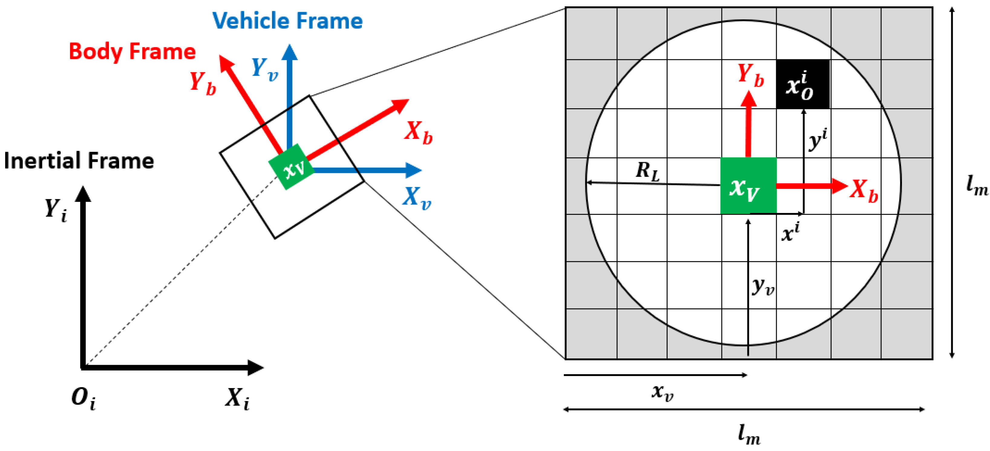
3.2. AGPF for Local Path Planning

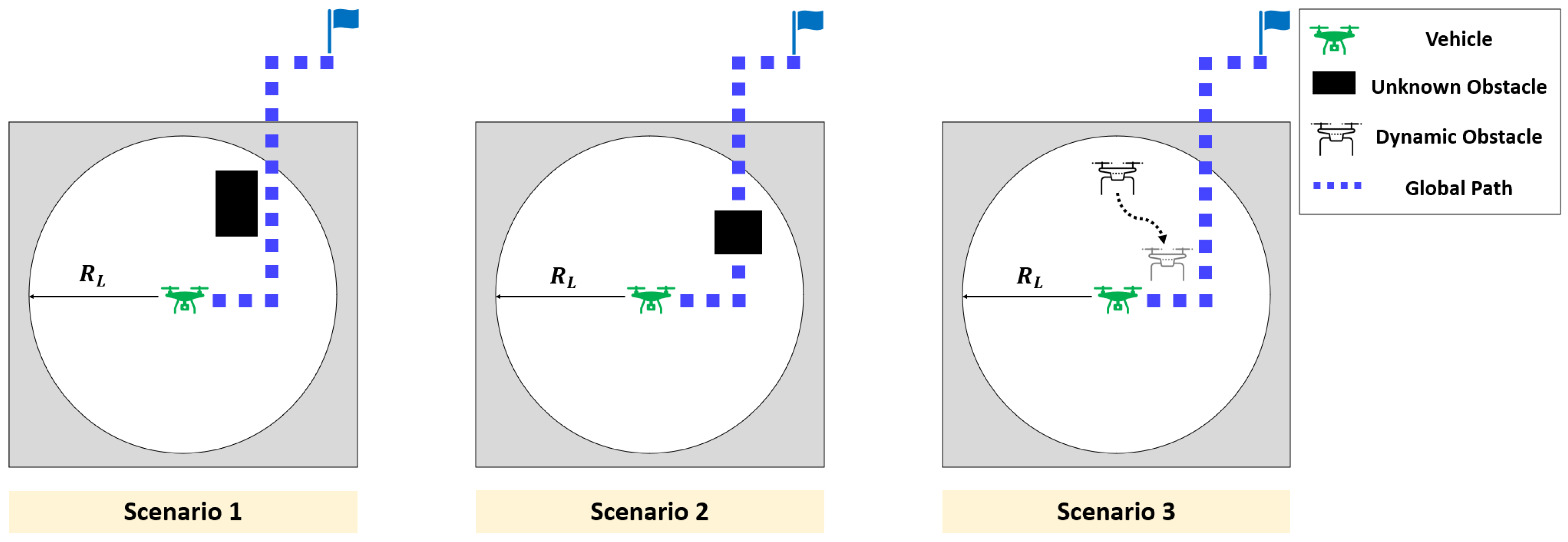
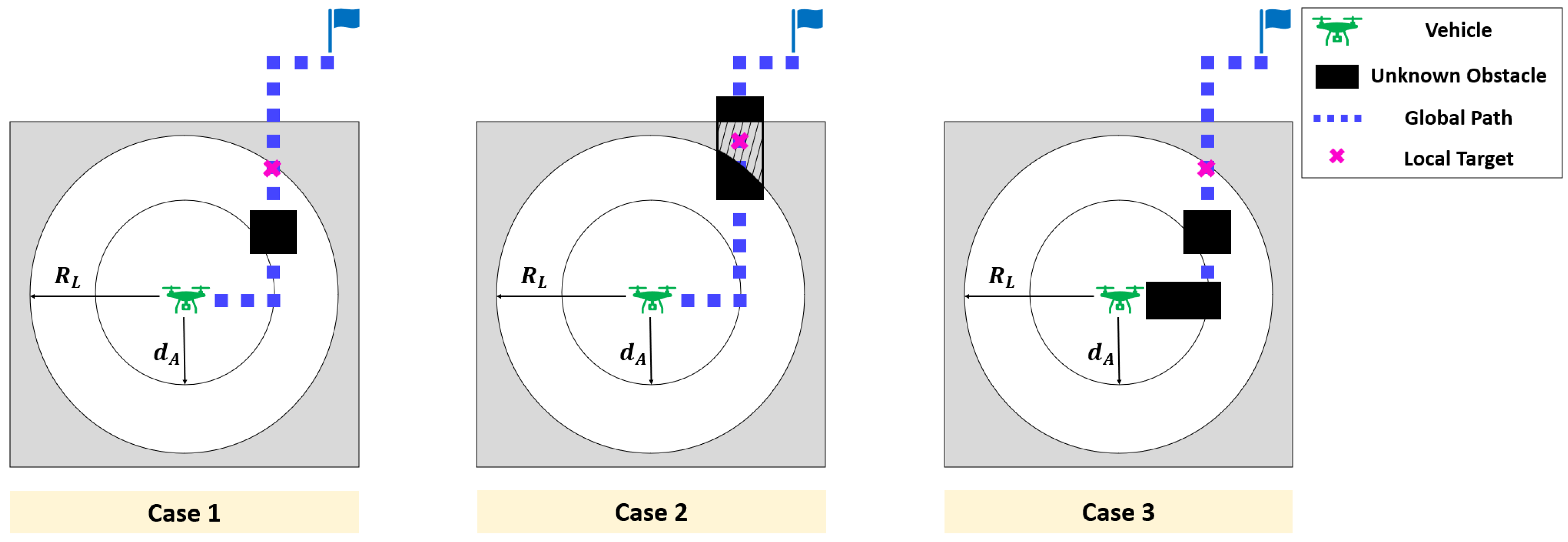
3.2.1. Avoidance of Obstacle

For collision-free navigation, the vehicle must be able to interpret the global path in conjunction with real-time environmental data acquired from onboard sensors, and dynamically generate and track a local path accordingly. In local path planning, the AGPF algorithm utilizes a grid map that reflects the surrounding environmental information of the vehicle, as shown in Figure 8.

The size of the grid map, $l_m$, is defined such that

$$l_m>2R_L$$

(16)

where $R_L$ is the detection range of the sensor. The grid map is fixed to the body frame of the vehicle, with the vehicle’s position $(x_v,y_v)$ always located at the center of the map. The relative position of an obstacle with respect to the vehicle is denoted as $(x^i,y^i)$, and the corresponding position of the obstacle on the map is determined using Equation (17).

$$x_o^i=x_v+x^i,y_o^i=y_v+y^i$$

(17)

Obstacles are visualized only within the sensor’s detection range, which corresponds to the white area of the grid map, while regions beyond this range (gray area) are not represented. The detected obstacle information within this range is then incorporated into the local path planning process.

The vehicle primarily follows the global path but switches to local path generation when new obstacles are detected by onboard sensors. The AGPF algorithm adapts its local path planning strategy according to the characteristics of the detected obstacles, which are classified into the following three scenarios, as illustrated in Figure 9.

In Scenario 1, unknown static obstacles are absent from the global path. Scenario 2 involves unknown static obstacles obstructing the global path, while Scenario 3 considers dynamic obstacles in the surrounding environment.

The local path generation method for Scenario 1 is described in Figure 10. Since the unknown obstacle is not located on the global path, there is no need to generate an entirely new path. Nevertheless, as the global path was planned without accounting for this obstacle, a potential risk of collision still exists. To address this, a local path is generated using the AGPF algorithm, which incorporates both the attractive force toward global waypoints within a specified range $d_G$ and the repulsive force from the detected obstacle. The parameter $d_G$ functions similarly to $d_A$, but it defines the distance at which the attractive force toward global waypoints begins to act, rather than A-star waypoints.

The local path generation method for Scenario 2, where an unknown static obstacle is located on the global path, is illustrated in Figure 11. If such an obstacle is detected, continuing along the original global path may lead to a collision. To avoid this, a new local path must be generated, beginning with the selection of a local target. This local target is not the final destination, but a temporary waypoint that guides the vehicle around the obstacle. It serves as a reference for constructing the avoidance path until the vehicle has safely bypassed the obstacle.

The procedure for selecting the local target is illustrated in Figure 12. If the detected obstacle is fully contained within the sensor’s detection range (white area), a global waypoint located behind the obstacle is selected as the local target, as shown in Case 1. However, if the obstacle is detected near the boundary of the sensor range, it may not be fully represented within the white area. In this case, selecting a waypoint behind the obstacle may be infeasible, as it lies outside the grid map. Instead, as shown in Case 2, a global waypoint located outside the sensor range but still within the grid map (gray area) is chosen as the local target. Since this region is unoccupied, it provides a valid reference point for path generation. Additionally, in situations involving multiple obstacles along the global path—as illustrated in Case 3—the algorithm selects a waypoint located behind the farthest obstacle from the vehicle. Once the local target is determined, an A-star path is generated toward it. The vehicle then constructs an AGPF-based local path by applying attractive forces toward the A-star waypoints within range $d_A$ and repulsive forces from the surrounding unknown obstacles.

Finally, the process for generating avoidance paths in Scenario 3, where dynamic obstacles are present around the vehicle, is illustrated in Figure 13. A local target is selected in a direction that facilitates safe avoidance of the dynamic obstacle. An A-star path is then computed toward this target, followed by the generation of an AGPF-based local path using attractive forces toward the A-star waypoints.

The effectiveness of dynamic obstacle avoidance heavily depends on how the local target is selected; thus, developing a reliable target selection strategy is essential. In this context, it is assumed that the vehicle has access to both the position and velocity of the dynamic obstacle. The dynamic repulsive field generated as the obstacle approaches the vehicle with a relative velocity is illustrated in Figure 14 and defined in Equation (18).

$$\begin{array}{cc}\hfill U_{DO}({\mathit{\rho }}_{DO},{\mathit{v}}_{VDO})& =\left\{\begin{array}{cc}cos\left({\theta }_i\right)\hfill & \mathrm{if}{d}_{DO}\le \parallel {\mathit{\rho }}_{DO}\parallel ,0\le {\theta }_i\le {\displaystyle \frac{\pi }{2}}\hfill \\ 0\hfill & \mathrm{if}\parallel {\mathit{\rho }}_{DO}\parallel <d_{DO}\hfill \end{array}\right.\hfill \end{array}$$

(18)

$$\begin{array}{c}\hfill with{\mathit{\rho }}_{DO}={\mathsf{x}}_i-{\mathsf{x}}_{DO},{\theta }_i={cos}^{-1}\left({\displaystyle \frac{{\mathit{v}}_{VDO}·{\mathit{\rho }}_{DO}}{\parallel {\mathit{v}}_{VDO}\parallel \parallel {\mathit{\rho }}_{DO}\parallel }}\right),i=1,2,\dots ,n\end{array}$$

where ${\mathit{x}}_{DO}$ is the position vector of the dynamic obstacle; ${\mathit{v}}_{DO}$ and ${\mathit{v}}_V$ represent velocity vectors of the dynamic obstacle and vehicle, respectively; ${\mathit{v}}_{VDO}$ is the relative velocity between the dynamic obstacle and the vehicle; ${\mathit{x}}_i$ denotes the position vector of the $i_{th}$ node out of the total n nodes on the grid map; ${\mathit{\rho }}_{DO}$ is the vector directed from the dynamic obstacle to the $i_{th}$ node; ${\theta }_i$ represents the angle between ${\mathit{\rho }}_{DO}$ and ${\mathit{v}}_{VDO}$; $d_{DO}$ is the distance set to prevent collisions between the vehicle and the obstacle.

The vehicle determines the local target based on a potential field that reflects the relative velocity between itself and the dynamic obstacle. If the vehicle is located within a region of the dynamic repulsive field where the potential value is negative, it implies that the obstacle is moving away, and no avoidance maneuver is necessary. In contrast, a positive potential value indicates that the obstacle is approaching, thereby requiring the generation of an avoidance path. To avoid the dynamic obstacle, the vehicle selects a target in the direction where the potential value decreases from its current position. As illustrated in Figure 15, the potential values are evaluated along a circular arc at a distance $d_m$ from the vehicle, and the point with the minimum potential is chosen as the local target. The position of the selected target, ${\mathit{x}}_L$, is given by Equation (19).

$${\mathsf{x}}_L={\mathsf{x}}_V+arg\underset{{\mathit{\rho }}_V}{min}\left(U_{DO}({\mathit{\rho }}_{DO},{\mathit{v}}_{VDO})\ne 0\mid \parallel {\mathit{\rho }}_V\parallel =d_m,{\mathit{\rho }}_V·{\mathit{v}}_V\ge 0\right)$$

(19)

$$\begin{array}{c}\hfill with{d}_m\ll R_L,{\mathit{\rho }}_V={\mathsf{x}}_i-{\mathsf{x}}_V\end{array}$$

As illustrated in Figure 16, setting the local target in a direction that forms a large angle with the vehicle’s velocity vector can lead to abrupt changes in heading, potentially compromising maneuvering stability. To mitigate such sudden directional changes, a constraint is applied to the angle between the velocity direction and the local target, as defined in Equation (20).

$${\mathsf{x}}_L=\left\{\begin{array}{cc}{\mathsf{x}}_V+{\mathbf{R}}_{\alpha c}{\mathsf{x}}_{LV}\hfill & c\le \alpha \hfill \\ {\mathsf{x}}_L\hfill & c>\alpha \hfill \end{array}\right.$$

(20)

where ${\mathit{x}}_{LV}$ is the vector from ${\mathit{x}}_V$ to ${\mathit{x}}_L$; $\alpha$ is the angle between ${\mathit{x}}_{LV}$ and ${\mathit{v}}_V$; ${\mathit{R}}_{\alpha c}$ is the rotation matrix used to transform the local target forming an angle $\alpha$ with the vehicle’s velocity into the local target forming an angle c with the vehicle’s velocity.

To address this issue, an additional virtual force, ${\mathit{F}}_V$, is introduced in the direction of the vehicle’s current velocity, as defined in Equation (21) and illustrated in Figure 17. This force, aligned with the vehicle’s flight direction, promotes smooth transitions and enhances path continuity across planning cycles.

$${\mathit{F}}_{Tot}={\mathit{F}}_{Att}+{\mathit{F}}_{Rep}+{\mathit{F}}_V=\sum _{j=1}^M{\mathit{F}}_A^j+\sum _{i=1}^N{\mathbf{F}}_O^{\prime i}+K_V{\displaystyle \frac{{\mathit{v}}_V}{\parallel {\mathit{v}}_V\parallel }}$$

(21)

where $K_V$ is the coefficient of the force in the direction of velocity.

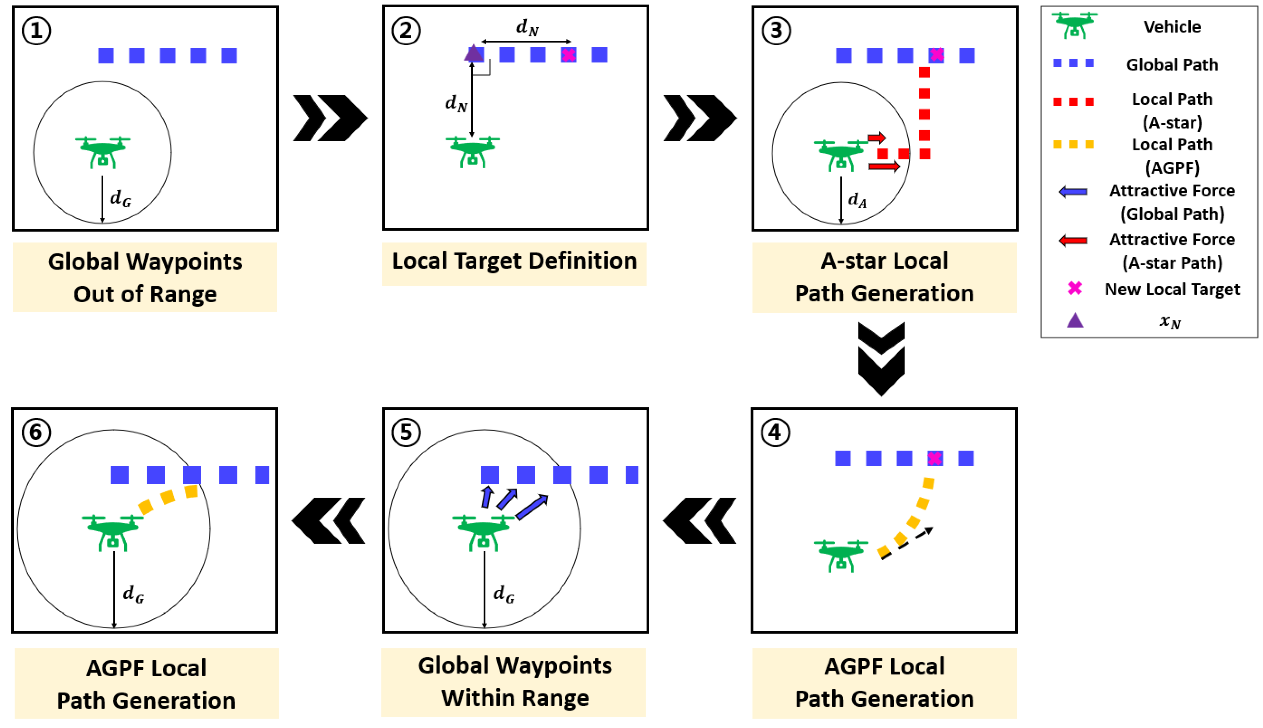
3.2.2. Return to Global Path

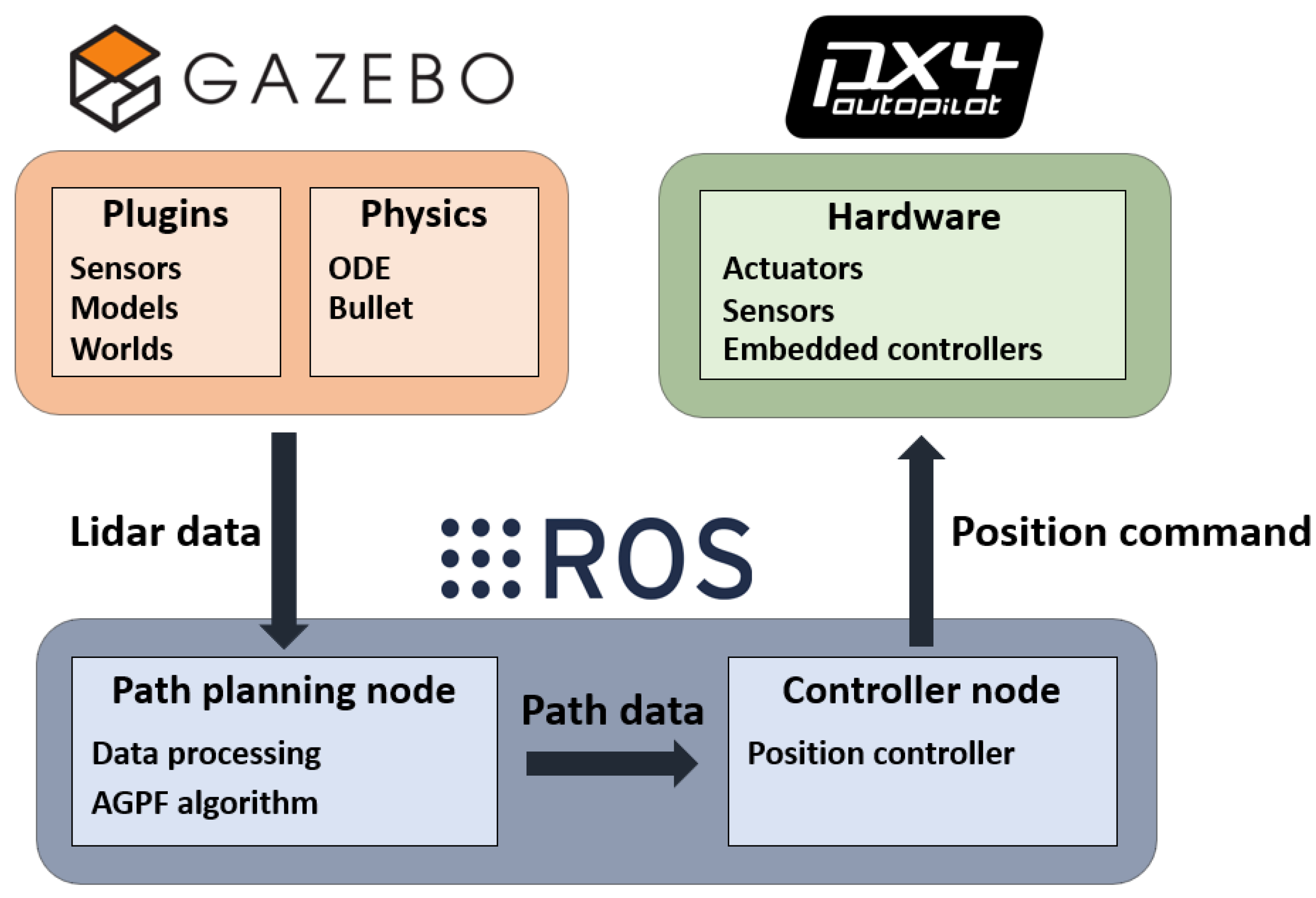
To avoid unknown or dynamic obstacles, the vehicle may temporarily deviate from the global path. Nonetheless, since the global path is preplanned with considerations for optimality, safety, and mission constraints, such deviations may lead to long-term inefficiencies or increased collision risks—especially when operating outside the designated area. Consequently, returning to the global path is essential to maintain overall path consistency and safety. The procedure for rejoining the global path is described in Figure 18.

If the global waypoints lie within the distance threshold $d_G$, an AGPF-based local path can be generated using attractive forces directed toward those waypoints, as illustrated in Figure 10. In contrast, when the global waypoints are located beyond $d_G$, the lack of an attractive force prevents local path formation. To address this, a point on the global path is selected as a new local target, enabling the vehicle to generate a path that guides it back toward the global path.

Let $x_N$ denote the point on the global path closest to the vehicle, and let $d_N$ be the distance between the vehicle and $x_N$. A local target is then selected on the global path at a distance of approximately $d_N$ from $x_N$. This distance does not need to be exact and can be adjusted based on mission requirements. Setting the target farther from $x_N$ increases the return time but enhances stability by reducing abrupt heading changes. Conversely, placing it closer shortens the return time but may degrade maneuverability due to sharper turns. Thus, the local target distance can be flexibly chosen to balance stability and responsiveness, depending on user intent and mission characteristics.

Once the local target is determined, an A-star path is generated toward it, as illustrated in Figure 11 and Figure 13. The vehicle then follows an AGPF-based local path constructed using attractive forces toward the A-star waypoints. As the vehicle approaches the global path and the global waypoints enter the range $d_G$, the A-star path generation is terminated. From that point onward, the AGPF path is generated using attractive forces directed toward the global waypoints within $d_G$.

4. Simulation

To validate the performance of the proposed AGPF algorithm, simulations were conducted in the ROS (Noetic) and Gazebo (v11) environments. The simulations were executed on a system equipped with an Intel Core i7-11700K processor running at 3.6 GHz and 32 GB of memory. The evaluation includes both global and local path planning scenarios, demonstrating the algorithm’s effectiveness in generating smooth, collision-free paths while responding to static and dynamic obstacles.

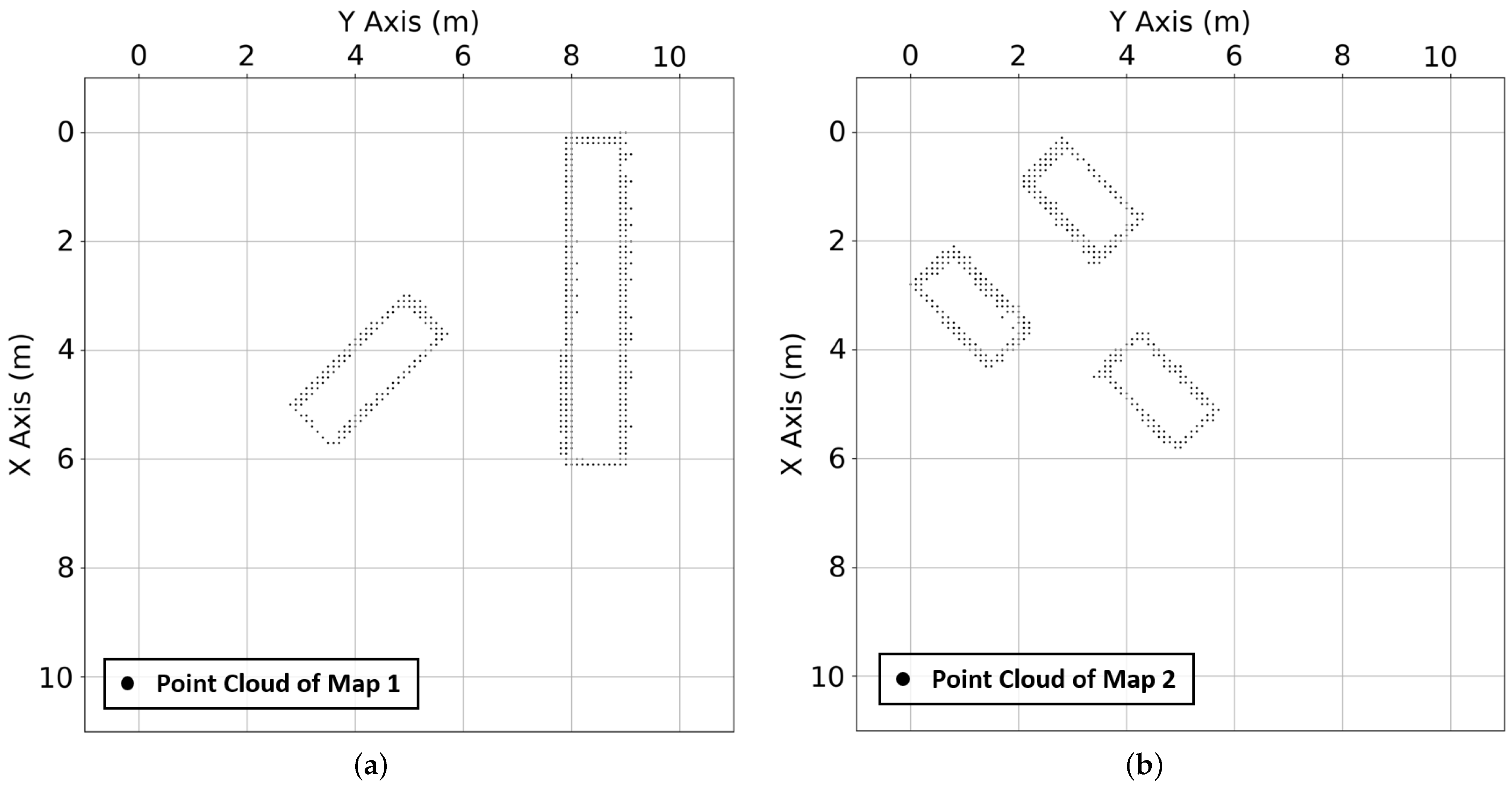
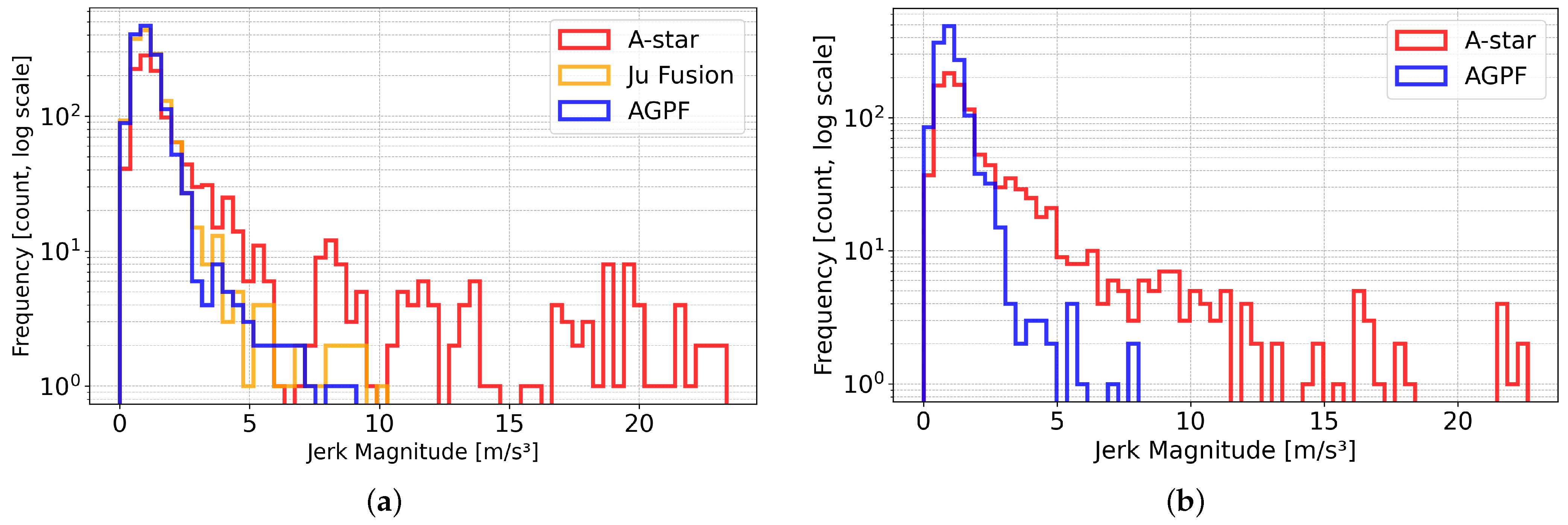
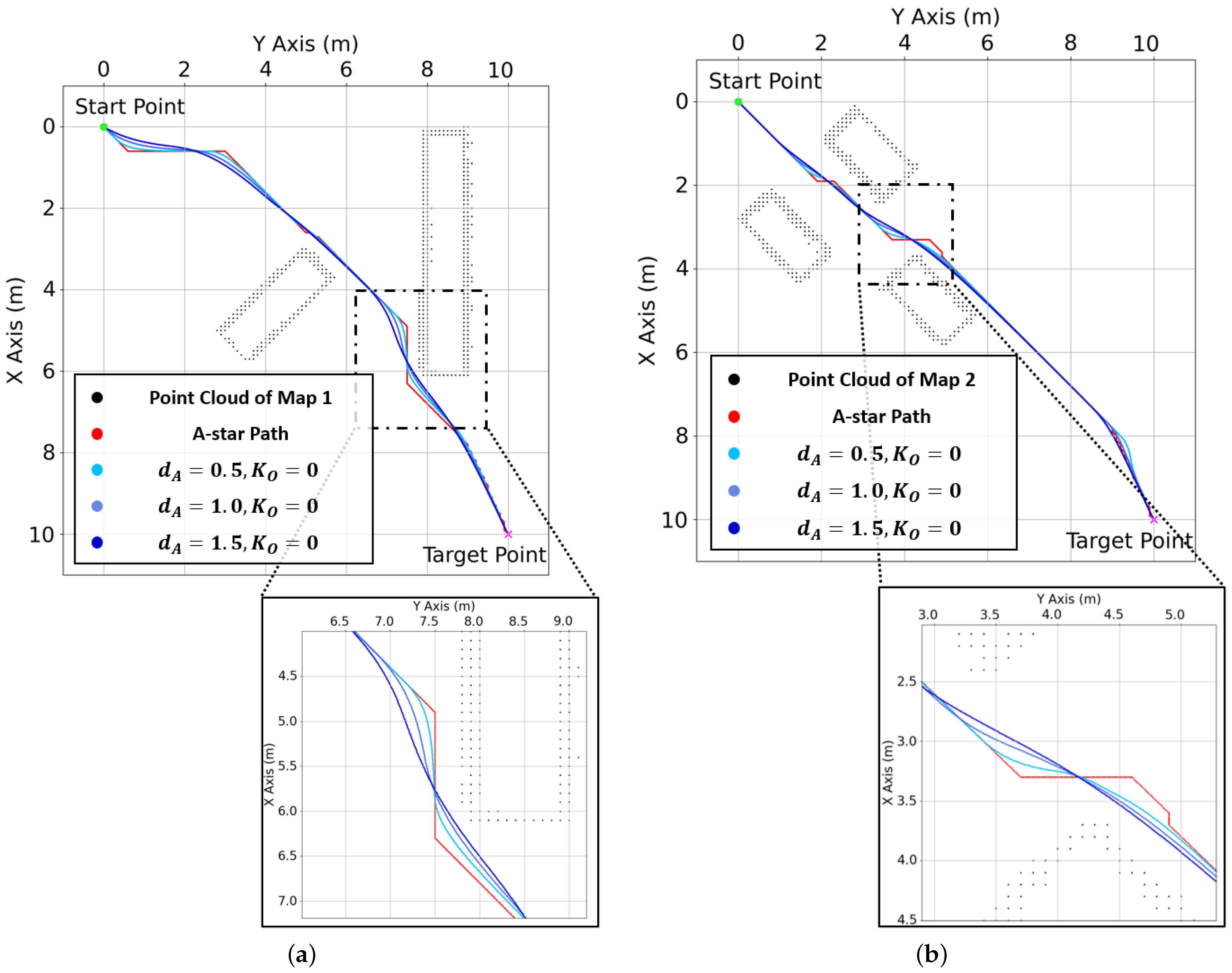
4.1. Global Path Planning

For global path planning, approximate environmental information about the mission area is typically required beforehand. A common and effective source of such information is point cloud data, which offers a detailed spatial representation of the terrain. In practice, approximate point cloud data for a given flight area can be obtained from open-access platforms such as OpenTopography or the National Ecological Observatory Network (NEON), both of which provide geospatial datasets for research and simulation purposes.

In this simulation, the UAV’s mission environment is shown in Figure 19, with corresponding point cloud data assumed to be available, as depicted in Figure 20. In this study, the point cloud data used for global path planning was generated by manually flying a UAV equipped with a simulated LiDAR sensor in the Gazebo environment, replicating realistic terrain scanning. It has a spatial resolution of 10 cm and is used to generate paths from the start point $(0,0,3)$ to the target $(10,10,3)$ using the A-star, APF, and AGPF algorithms. The parameters used for each algorithm are summarized in

Table 1. Coefficients for each algorithm.

Coefficient	A-Star	APF	Ju’s Fusion	AGPF	Unit
Grid size	0.1	-	0.1	0.1	m
$K_G$	-	10	-	-	-
$K_O$	-	1	1	1	-
$l_O$	-	1.5	1.5	1.5	-
$d_O$	-	1.5	1.5	1.5	m
$K_A$	-	-	20	20	-
$d_A$	-	-	1	1	m
$\delta$	0.01	0.01	0.01	0.01	m

, and the resulting global path planning outcomes are presented in Figure 21.

To evaluate the smoothness of the global path, a jerk distribution histogram based on the global path can be obtained, as shown in Figure 22.

As shown in Figure 21, the A-star algorithm successfully generates paths to the target in both map scenarios. However, the resulting paths exhibit abrupt directional changes, as indicated by the high jerk magnitudes in the histogram. This reduced smoothness may pose challenges for the vehicle’s path-following controller, potentially affecting tracking accuracy and stability. In contrast, the APF algorithm fails to generate a complete path in either map, as depicted in Figure 21a. In this case, the vehicle, obstacle, and target are aligned, causing the attractive force to be blocked by the obstacle and preventing progress. Figure 21b illustrates another failure scenario in which the vehicle attempts to pass between two obstacles; the overlapping repulsive forces cancel out the attractive force, resulting in a local minimum and halting path generation.

Ju’s fusion algorithm successfully generates a path to the target in Map 1 by refining the trajectory obtained from the A-star algorithm. The corresponding jerk histogram further confirms that the resulting trajectory is smoother than that of A-star. However, in Map 2, the algorithm fails to complete the path due to the influence of the repulsive force component ${\mathit{F}}_{OP}$, which counteracts the attractive force and results in a local minimum. In contrast, the proposed AGPF algorithm effectively addresses the limitations of both the APF and Ju’s fusion algorithm by generating collision-free trajectories that avoid local minima. It builds upon the A-star path and refines it using a modified potential field formulation. As shown in Figure 21a, AGPF effectively avoids obstacles that block the attractive force toward the target, allowing the vehicle to continue without becoming trapped. In Figure 21b, the modified force formulation prevents the net force from reaching zero, enabling the vehicle to navigate between closely spaced obstacles. As shown in the jerk histogram, the AGPF algorithm generates smoother and more naturally curved trajectories compared to the A-star algorithm, effectively reducing abrupt directional changes and enabling safer obstacle avoidance. As presented in

Table 2. Path length for each algorithm.

Map	Data	A-star	APF	Ju’s Fusion	AGPF	Unit
Map 1	Path length	15.665	-	15.090	15.050	m
	Time	0.409	-	3.309	3.313	s
Map 2	Path length	14.904	-	-	14.470	m
	Time	0.171	-	-	2.714	s

, this also results in a shorter overall path length than that of the A-star algorithm.

The AGPF algorithm introduces a new coefficient, $d_A$, which is not present in the conventional APF. To evaluate its effect on path planning, simulations were conducted with varying $d_A$ values while setting the repulsive coefficient $K_O$ to 0. The results, shown in Figure 23, indicate that smaller $d_A$ values produce paths that closely resemble those of the A-star algorithm, whereas larger $d_A$ values result in smoother, more curved trajectories. Although increased smoothness helps reduce abrupt heading changes and improves path-following performance, excessively large $d_A$ values may lead to paths that are overly curved and potentially closer to obstacles. Hence, the value of $d_A$ should be carefully adjusted according to environmental conditions and mission requirements.

4.2. Local Path Planning

The local path planning simulations utilize the PX4-Autopilot Iris drone, which is equipped with a LiDAR sensor to collect real-time data on surrounding obstacles. A grid map satisfying the condition in Equation (16) is constructed for path generation, with the detected obstacle information visualized on the map, as shown in Figure 24. Detailed specifications of the LiDAR sensor and the grid map are summarized in

Table 3. Information about LiDAR and grid map.

Coefficient	LiDAR and Grid Map	Unit
Range $\left(R_L\right)$	5	m
Range resolution	0.1	m
$l_m$	11	m
Min angle and Max angle	−180 and 180	deg
Horizontal resolution	1	deg
Grid size	0.1	m

.

In the grid map, black-filled cells indicate the actual positions of obstacle point clouds detected by the sensor, while gray-filled cells represent a protective zone added to prevent potential collisions. Although the gray area does not correspond to physical obstacles, it is incorporated to ensure a safe flight margin. During A-star path planning, the vehicle accounts for both the actual obstacles and the protective zones to compute a collision-free path.

The local path planning maps are derived from those shown in Figure 19, with the addition of unknown obstacles for real-time avoidance scenarios. As illustrated in Figure 25, green rectangular pillars represent predefined static obstacles known prior to the mission, while red cylindrical pillars denote unknown static obstacles that must be detected and avoided by the vehicle during flight.

The vehicle generates local paths in real time at a frequency of 2 Hz, using its current position and surrounding obstacle information. The AGPF algorithm is employed for local path planning, with its parameters listed in

Table 4. Coefficients for AGPF algorithm.

Coefficient	AGPF	Unit
Grid size	0.1	m
Local path length	0.8	m
$K_O$	1	-
$l_O$	1.5	-
$d_O$	1.5	m
$K_A$	2	-
$d_A$	1	m
$\delta$	0.01	m
$K_{DO}$	10	-
$d_m$	0.8	m
$d_{DO}$	1	m
c	30	deg
$K_V$	0.5	-

. The resulting path is transmitted to the vehicle as position commands, which are executed by the position-based controller integrated into the PX4-Autopilot. The overall system architecture is illustrated in Figure 26.

The proposed system integrates Gazebo, ROS, and PX4-Autopilot to form a closed-loop UAV simulation environment. In this setup, the Gazebo simulator collects real-time environmental data via a LiDAR sensor, which is transmitted to the path planning node in ROS. This node processes the sensor data and generates a collision-free path using the AGPF algorithm. The resulting path is published through a ROS topic and received by the controller node, which computes the corresponding position commands for the UAV. These commands are then delivered to the PX4-Autopilot’s position controller, enabling real-time vehicle control.

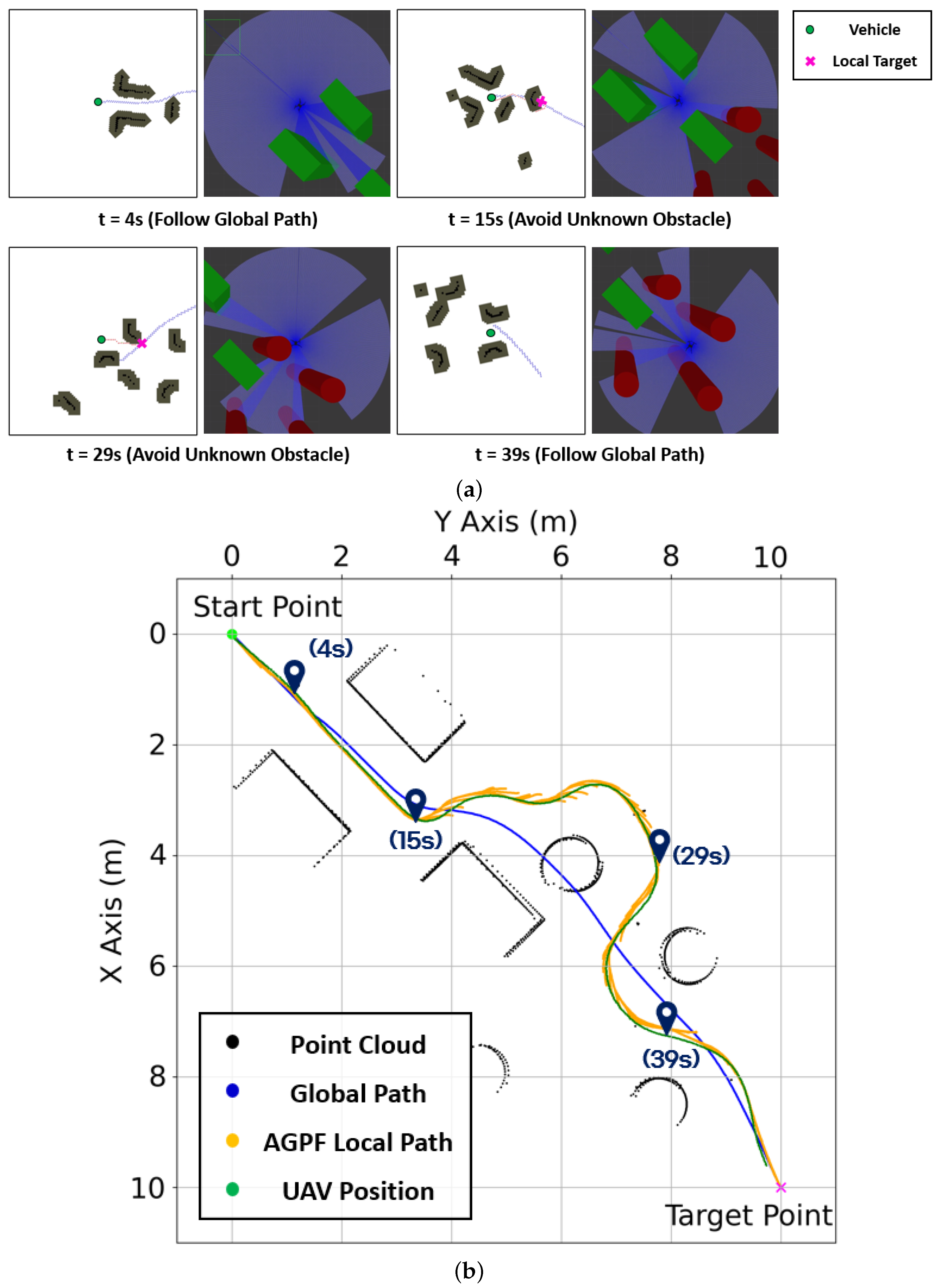
4.2.1. Avoidance of Unknown Obstacle

The simulation results of the AGPF algorithm applied to Map 3 are presented in Figure 27. Figure 27a illustrates the process in which the UAV selects a local target at specific time steps and generates an A-star path (red dots), with the predefined global path also shown in blue. The corresponding AGPF trajectories along with the UAV’s actual flight path are visualized in Figure 27b. At 5 s, the UAV detected an unknown obstacle on the global path and selected a global waypoint behind the obstacle as the local target. An A-star path was generated toward this point, followed by an AGPF-based path for obstacle avoidance. By 15 s, the obstacle had been successfully bypassed, allowing the UAV to resume path generation based on global waypoints within the range $d_G$. At 22 s, another unknown obstacle was detected, and from 22 to 36 s, the UAV again generated and followed an AGPF-based local path to avoid it.

The simulation results of the AGPF algorithm applied to Map 4 are presented in Figure 28. From 0 to 4 s, the UAV generated local paths toward global waypoints within the range $d_G$. After 4 s, an unknown obstacle was detected on the global path, prompting the UAV to generate an A-star path followed by an AGPF-based local path. At 29 s, the UAV encountered two additional unknown obstacles and selected a point behind the farthest one as the local target. Based on this target, an A-star path was generated, and the UAV performed obstacle avoidance for 39 s. Afterward, with the global waypoints again within the range $d_G$, the UAV resumed AGPF-based path generation toward the global path.

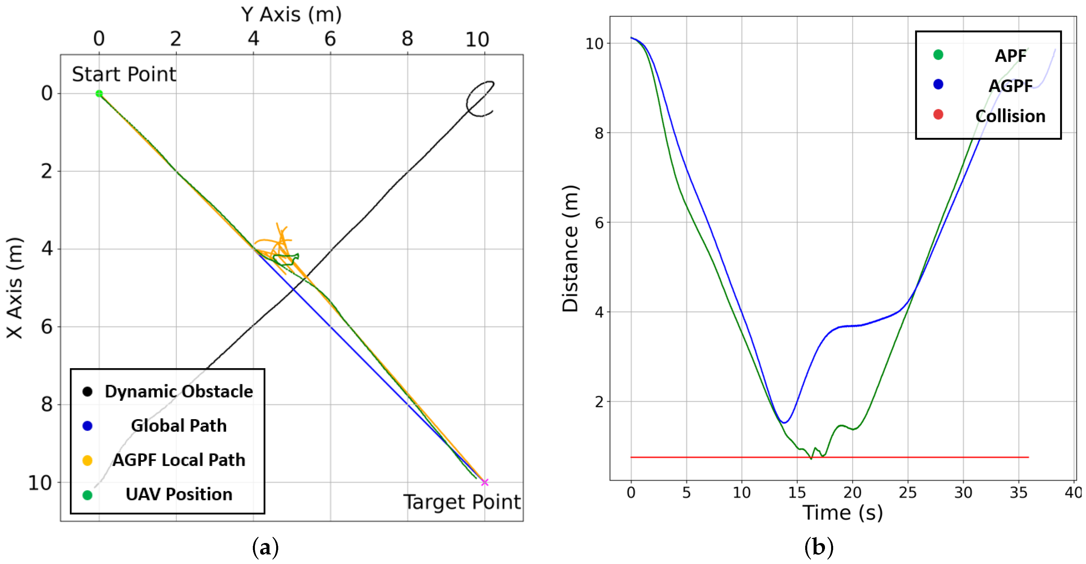
4.2.2. Avoidance of Dynamic Obstacle

Dynamic obstacle avoidance was evaluated through simulations in two Test Scenarios. In Test Scenario 1, a dynamic obstacle approaches the vehicle head-on at the same speed, while in Test Scenario 2, the obstacle approaches from a diagonal direction. The performance of the AGPF algorithm was compared with that of the APF algorithm, using the coefficients listed in Table 1. The simulation results for the first scenario, where the obstacle approaches from the front, are presented in Figure 29.

As shown in the simulation results, the UAV began responding to the dynamic repulsive field at 13 s, with a positive potential value indicating that the obstacle was approaching. From 13 to 17 s, the UAV selected a local target in the direction of decreasing potential, enabling successful avoidance. By 18 s, the potential value turned negative, signaling completion of the avoidance maneuver. At that point, the dynamic obstacle was located on the global path. Between 18 and 20 s, the UAV selected a waypoint behind the obstacle as a local target and followed an AGPF-based path to navigate around it. After 20 s, with the dynamic obstacle no longer present and the global waypoints located outside the range $d_G$, the UAV returned to the global path using the method described in Figure 18. As illustrated in Figure 29b, the AGPF-generated path remained smooth and continuous throughout the maneuver, allowing effective tracking while avoiding the obstacle.

To validate the performance of the AGPF algorithm, the same scenario was tested using the APF algorithm, and the results are presented in Figure 30.

To further validate the performance of the AGPF algorithm, the same scenario was simulated using the conventional APF algorithm, with the results shown in Figure 30. As illustrated in Figure 30a, the APF-generated local path is discontinuous and contains sharp turns, making it difficult for the vehicle to follow accurately. This degraded tracking performance can result in collisions. Figure 30b confirms this outcome, showing that the vehicle-obstacle distance falls below the collision threshold. In contrast, the AGPF maintains a safe separation from the obstacle, consistently keeping the vehicle-obstacle distance above the collision limit and avoiding contact.

The simulation results for the scenario in which a dynamic obstacle approaches from a diagonal direction are presented in Figure 31. Between 12 and 17 s, the potential value of the dynamic repulsive field at the UAV’s position remained positive, prompting the UAV to select local targets that guided it along a direction of decreasing potential. At 18 s, the potential value turned negative, indicating successful avoidance. At this point, the dynamic obstacle was located on the global path, and the UAV selected a waypoint behind it as the local target, following an AGPF-based local path to navigate around the obstacle. After 22 s, with the global waypoints falling within the range $d_G$, the UAV resumed AGPF-based local path generation toward the global path. As shown in Figure 31b, the resulting path was smooth and continuous, enabling the UAV to effectively avoid the dynamic obstacle. For comparison, the simulation result using the APF algorithm is shown in Figure 32.

As shown in Figure 32a, the APF-generated local path is difficult for the vehicle to follow due to its abrupt changes and discontinuities. As a result, the vehicle-obstacle distance falls below the collision threshold, leading to a collision, as illustrated in Figure 32b. In contrast, the AGPF algorithm maintains a safe distance above the collision threshold, effectively preventing collisions.

5. Conclusions

This paper proposes a UAV path planning framework that divides the navigation process into global and local planning stages, introducing a novel algorithm—A-star-Guided Potential Field (AGPF)—that combines the strengths of the A-star and Artificial Potential Field (APF) methods. The conventional A-star algorithm guarantees path optimality but is computationally demanding and often produces unsmooth trajectories, making it less suitable for real-time applications or for use with actual flight platforms. In contrast, the APF algorithm offers smooth and computationally efficient path generation but suffers from local minima and lacks path optimality. Both algorithms also have limited capability in handling moving obstacles. AGPF addresses these limitations by integrating the optimal path structure of A-star with the smooth trajectory characteristics of APF, while incorporating a modified force model and a waypoint-based attractive field. This allows AGPF to avoid local minima and maintain trajectory continuity, especially in complex environments. In global path planning, AGPF applies attractive forces to A-star waypoints, thereby preserving optimality while smoothing the path. In local path planning, three scenarios are considered: the presence of unknown obstacles off the global path, on the global path, and the presence of dynamic obstacles. For each case, dedicated avoidance strategies and recovery mechanisms are proposed to guide the vehicle safely and efficiently back to the global path. The proposed algorithm was validated through simulations in ROS and Gazebo environments. Results demonstrated that AGPF outperforms the conventional APF algorithm in terms of real-time path generation, smoothness, and obstacle avoidance performance.

The current simulation results are based on an ideal environment where sensor noise from LiDAR and GNSS/IMU is not considered. In real-world applications, however, such noise can significantly impact system performance, necessitating further validation to assess the robustness of the proposed algorithm. Additionally, when a UAV operates over uneven or undulating terrain, altitude control and full 3D path planning become essential. Since the AGPF algorithm is developed within a 2D planning framework, it has inherent limitations in handling vertical obstacle avoidance and adapting to complex topographical variations.

Although the use of the A-star algorithm within AGPF enables fast computation in 2D local path planning, it suffers from scalability issues in 3D environments due to the curse of dimensionality, limiting its real-time applicability. Furthermore, while AGPF generates relatively smooth trajectories compared to traditional grid-based methods, the resulting paths do not account for UAV-specific flight dynamics such as turning radius and velocity constraints. As a result, despite improved path smoothness, AGPF trajectories may still fall short of being directly executable in real UAV flight scenarios.

To address these limitations, future work will incorporate filter-based obstacle position estimation to improve robustness under sensor noise. For local path planning, the A-star algorithm will be replaced with the more computationally efficient D-star lite algorithm, which is better suited for real-time applications and will be extended to support 3D path planning. In addition, the APF component of AGPF will be refined to generate dynamically feasible trajectories that consider the UAV’s motion constraints. A Model Predictive Control (MPC)-based flight controller will also be developed to enhance trajectory tracking accuracy. Ultimately, these advancements will be validated through hardware-in-the-loop simulations and real-world experiments using an actual UAV platform.

References

1. Davies, S.; Pettersson, T.; Öberg, M. Organized violence 1989–2021 and drone warfare. J. Peace Res. 2022, 59, 593–610. [Google Scholar] [CrossRef]
2. Xiaoning, Z. Analysis of military application of UAV swarm technology. In Proceedings of the 2020 3rd International Conference on Unmanned Systems (ICUS), Harbin, China, 27–28 November 2020; pp. 1200–1204. [Google Scholar]
3. Daud, S.M.S.M.; Yusof, M.Y.P.M.; Heo, C.C.; Khoo, L.S.; Singh, M.K.C.; Mahmood, M.S.; Nawawi, H. Applications of drone in disaster management: A scoping review. Sci. Justice 2022, 62, 30–42. [Google Scholar] [CrossRef]
4. Mishra, B.; Garg, D.; Narang, P.; Mishra, V. Drone-surveillance for search and rescue in natural disaster. Comput. Commun. 2020, 156, 1–10. [Google Scholar] [CrossRef]
5. Kunertova, D. The war in Ukraine shows the game-changing effect of drones depends on the game. Bull. At. Sci. 2023, 79, 95–102. [Google Scholar] [CrossRef]
6. Abrahamsen, H.B. A remotely piloted aircraft system in major incident management: Concept and pilot, feasibility study. BMC Emerg. Med. 2015, 15, 1–12. [Google Scholar] [CrossRef]
7. Seguin, C.; Blaquière, G.; Loundou, A.; Michelet, P.; Markarian, T. Unmanned aerial vehicles (drones) to prevent drowning. Resuscitation 2018, 127, 63–67. [Google Scholar] [CrossRef] [PubMed]
8. Anwar, N.; Izhar, M.A.; Najam, F.A. Construction monitoring and reporting using drones and unmanned aerial vehicles (UAVs). In Proceedings of the Tenth International Conference on Construction in the 21st Century (CITC-10), Colombo, Sri Lanka, 2–4 July 2018; Volume 8, pp. 2–4. [Google Scholar]
9. Mangiameli, M.; Muscato, G.; Mussumeci, G.; Milazzo, C. A GIS application for UAV flight planning. IFAC Proc. Vol. 2013, 46, 147–151. [Google Scholar] [CrossRef]
10. Hart, P.E.; Nilsson, N.J.; Raphael, B. A formal basis for the heuristic determination of minimum cost paths. IEEE Trans. Syst. Sci. Cybern. 1968, 4, 100–107. [Google Scholar] [CrossRef]
11. Tang, G.; Tang, C.; Claramunt, C.; Hu, X.; Zhou, P. Geometric A-star algorithm: An improved A-star algorithm for AGV path planning in a port environment. IEEE Access 2021, 9, 59196–59210. [Google Scholar] [CrossRef]
12. Erke, S.; Bin, D.; Yiming, N.; Qi, Z.; Liang, X.; Dawei, Z. An improved A-Star based path planning algorithm for autonomous land vehicles. Int. J. Adv. Robot. Syst. 2020, 17, 1729881420962263. [Google Scholar] [CrossRef]
13. Li, J.; Liao, C.; Zhang, W.; Fu, H.; Fu, S. UAV path planning model based on R5DOS model improved A-star algorithm. Appl. Sci. 2022, 12, 11338. [Google Scholar] [CrossRef]
14. Stentz, A. Optimal and efficient path planning for partially-known environments. In Proceedings of the 1994 IEEE International Conference on Robotics and Automation, San Diego, CA, USA, 8–13 May 1994; pp. 3310–3317. [Google Scholar]
15. Stentz, A. The focussed d* algorithm for real-time replanning. In Proceedings of the International Joint Conference on Artificial Intelligence, Montreal, QC, Canada, 20–25 August 1995; Volume 95, pp. 1652–1659. [Google Scholar]
16. Koenig, S.; Likhachev, M.; Furcy, D. Lifelong planning A. Artif. Intell. 2004, 155, 93–146. [Google Scholar] [CrossRef]
17. Koenig, S.; Likhachev, M. Fast replanning for navigation in unknown terrain. IEEE Trans. Robot. 2005, 21, 354–363. [Google Scholar] [CrossRef]
18. Guan, W.; Wang, K. Autonomous collision avoidance of unmanned surface vehicles based on improved A-star and dynamic window approach algorithms. IEEE Intell. Transp. Syst. Mag. 2023, 15, 36–50. [Google Scholar] [CrossRef]
19. Liao, T.; Chen, F.; Wu, Y.; Zeng, H.; Ouyang, S.; Guan, J. Research on Path Planning with the Integration of Adaptive A-Star Algorithm and Improved Dynamic Window Approach. Electronics 2024, 13, 455. [Google Scholar] [CrossRef]
20. He, Z.; Liu, C.; Chu, X.; Negenborn, R.R.; Wu, Q. Dynamic anti-collision A-star algorithm for multi-ship encounter situations. Appl. Ocean Res. 2022, 118, 102995. [Google Scholar] [CrossRef]
21. Nash, A.; Daniel, K.; Koenig, S.; Felner, A. Theta*: Any-angle path planning on grids. In Proceedings of the Twenty-Second Conference on Artificial Intelligence, Vancouver, BC, Canada, 22–26 July 2007; Volume 7, pp. 1177–1183. [Google Scholar]
22. Liu, Y.; Wang, L. AGV Path Planning: An Improved A* Algorithm Based on Bézier Curve Smoothing. In Proceedings of the 2024 39th Youth Academic Annual Conference of Chinese Association of Automation (YAC), Dalian, China, 7–9 June 2024; pp. 243–247. [Google Scholar]
23. Jayaweera, H.M.; Hanoun, S. Path planning of unmanned aerial vehicles (UAVs) in windy environments. Drones 2022, 6, 101. [Google Scholar] [CrossRef]
24. Aldao, E.; González-de Santos, L.M.; González-Jorge, H. LiDAR based detect and avoid system for UAV navigation in UAM corridors. Drones 2022, 6, 185. [Google Scholar] [CrossRef]
25. Du, Y.; Zhang, X.; Nie, Z. A real-time collision avoidance strategy in dynamic airspace based on dynamic artificial potential field algorithm. IEEE Access 2019, 7, 169469–169479. [Google Scholar] [CrossRef]
26. Rimon, E. Exact Robot Navigation Using Artificial Potential Functions; Yale University: New Haven, CT, USA, 1990. [Google Scholar]
27. Bounini, F.; Gingras, D.; Pollart, H.; Gruyer, D. Modified artificial potential field method for online path planning applications. In Proceedings of the 2017 IEEE Intelligent Vehicles Symposium (IV), Los Angeles, CA, USA, 11–14 June 2017; pp. 180–185. [Google Scholar]
28. Hao, G.; Lv, Q.; Huang, Z.; Zhao, H.; Chen, W. Uav path planning based on improved artificial potential field method. Aerospace 2023, 10, 562. [Google Scholar] [CrossRef]
29. Ruchti, J.; Senkbeil, R.; Carroll, J.; Dickinson, J.; Holt, J.; Biaz, S. Unmanned aerial system collision avoidance using artificial potential fields. J. Aerosp. Inf. Syst. 2014, 11, 140–144. [Google Scholar] [CrossRef]
30. Qixin, C.; Yanwen, H.; Jingliang, Z. An evolutionary artificial potential field algorithm for dynamic path planning of mobile robot. In Proceedings of the 2006 IEEE/RSJ International Conference on Intelligent Robots and Systems, Beijing, China, 9–13 October 2006; pp. 3331–3336. [Google Scholar]
31. Ge, S.S.; Cui, Y.J. Dynamic motion planning for mobile robots using potential field method. Auton. Robot. 2002, 13, 207–222. [Google Scholar] [CrossRef]
32. Sheng, J.; He, G.; Guo, W.; Li, J. An improved artificial potential field algorithm for virtual human path planning. In Proceedings of the Entertainment for Education. Digital Techniques and Systems: 5th International Conference on E-learning and Games, Edutainment 2010, Changchun, China, 16–18 August 2010; Proceedings 5. Springer: Berlin/Heidelberg, Germany, 2010; pp. 592–601. [Google Scholar]
33. Li, G.; Yamashita, A.; Asama, H.; Tamura, Y. An efficient improved artificial potential field based regression search method for robot path planning. In Proceedings of the 2012 IEEE International Conference on Mechatronics and Automation, Chengdu, China, 5–8 August 2012; pp. 1227–1232. [Google Scholar]
34. Ju, C.; Luo, Q.; Yan, X. Path planning using artificial potential field method and A-star fusion algorithm. In Proceedings of the 2020 Global Reliability and Prognostics and Health Management (PHM-Shanghai), Shanghai, China, 16–18 October 2020; pp. 1–7. [Google Scholar]
35. Liu, J.; Yan, Y.; Yang, Y.; Li, J. An improved artificial potential field UAV path planning algorithm guided by RRT under environment-aware modeling: Theory and simulation. IEEE Access 2024, 12, 12080–12097. [Google Scholar] [CrossRef]
36. Xu, D.; Yang, J.; Zhou, X.; Xu, H. Hybrid path planning method for USV using bidirectional A* and improved DWA considering the manoeuvrability and COLREGs. Ocean Eng. 2024, 298, 117210. [Google Scholar] [CrossRef]
37. Choi, J.W.; Choi, Y.H. Fusion Algorithm of A-star and Artificial Potential Field for Path Planning. In Proceedings of the 1st International Conference on on Drones and Unmanned Systems (DAUS’ 2025), Granada, Spain, 19–21 February 2025. [Google Scholar]
Figure 1. Path planning flow chart. Global path planning focuses on generating an optimal path based on static environmental data, whereas local path planning emphasizes real-time adaptation to dynamic environmental changes.
Drones 09 00545 g001
Figure 2. Sketch of the repulsive force. The repulsive force reaches its maximum at distance A; it increases as the obstacle approaches up to A, and decreases beyond A, depending on the distance to the obstacle.
Drones 09 00545 g002
Figure 3. Sketch forces at x in APF.
Drones 09 00545 g003
Figure 4. Examples of local minima in APF: (a) the obstacle blocks the vehicle’s path to the target; (b) the vehicle passes through a narrow space between obstacles.
Drones 09 00545 g004
Figure 5. Flow chart of AGPF.
Drones 09 00545 g005
Figure 6. Sketch virtual forces acting on the vehicle in AGPF: (a) the obstacle blocks the vehicle’s path to the target; (b) vehicle passes through a narrow space between obstacles.
Drones 09 00545 g006
Figure 7. Comparison of the traditional and modified repulsive forces.
Drones 09 00545 g007
Figure 8. Sketch a grid map.
Drones 09 00545 g008
Figure 9. The classification of an obstacle detected by the sensor.
Drones 09 00545 g009
Figure 10. The generation of a local path in Scenario 1 (non-blocking obstacle).
Drones 09 00545 g010
Figure 11. The generation of a local path in Scenario 2 (blocking obstacle).
Drones 09 00545 g011
Figure 12. Example of selecting a local target.
Drones 09 00545 g012
Figure 13. Generation of a local path in Scenario 3.
Drones 09 00545 g013
Figure 14. Sketch of the dynamic repulsive field.
Drones 09 00545 g014
Figure 15. Search of the local target.
Drones 09 00545 g015
Figure 16. Local target reset for minimizing sudden changes in the heading angle.
Drones 09 00545 g016
Figure 17. Description of a new attractive force.
Drones 09 00545 g017
Figure 18. The method for returning to the global path.
Drones 09 00545 g018
Figure 19. Global path planning simulation environment in Gazebo: (a) Map 1; (b) Map 2.
Drones 09 00545 g019
Figure 20. Point cloud representation of the simulation maps: (a) Map 1; (b) Map 2.
Drones 09 00545 g020
Figure 21. (a) Simulation results for Map 1; (b) simulation results for Map 2.
Drones 09 00545 g021
Figure 22. Comparison of jerk histograms for path planning algorithms: (a) histogram for Map 1; (b) histogram for Map 2.
Drones 09 00545 g022
Figure 23. (a) The effect of d A value in Map 1; (b) the effect of d A value in Map 2.
Drones 09 00545 g023
Figure 24. Detected obstacle displayed on the grid map.
Drones 09 00545 g024
Figure 25. Local path planning simulation environment in Gazebo: (a) Map 3; (b) Map 4.
Drones 09 00545 g025
Figure 26. System architecture integrating Gazebo, ROS, and PX4 autopilot.
Drones 09 00545 g026
Figure 27. (a) Time-based vehicle path generation in Map 3; (b) AGPF simulation result in Map 3.
Drones 09 00545 g027
Figure 28. (a) Time-based vehicle path generation in Map 4; (b) AGPF simulation result in Map 4.
Drones 09 00545 g028
Figure 29. (a) Time-based vehicle path generation in scenario 1; (b) AGPF simulation result in Test Scenario 1.
Drones 09 00545 g029
Figure 30. (a) APF simulation result in Test Scenario 1; (b) comparison of distance between dynamic obstacle in Test Scenario 1.
Drones 09 00545 g030
Figure 31. (a) Time-based vehicle path generation in Test Scenario 2; (b) AGPF simulation result in Test Scenario 2.
Drones 09 00545 g031
Figure 32. (a) APF simulation result in Test Scenario 2; (b) comparison of distance between dynamic obstacle in Test Scenario 2.
Drones 09 00545 g032