A Self-Adaptive Improved Slime Mold Algorithm for Multi-UAV Path Planning

Abstract

Multi-UAV path planning presents a critical challenge in Unmanned Aerial Vehicle (UAV) applications, particularly in environments with various obstacles and restrictions. These conditions transform multi-UAV path planning into a complex optimization problem with multiple constraints, significantly reducing the number of feasible solutions and complicating the generation of optimal flight trajectories. Although the slime mold algorithm (SMA) has proven effective in optimization missions, it still suffers from limitations such as inadequate exploration capacity, premature convergence, and a propensity to become stuck in local optima. These drawbacks degrade its performance in intricate multi-UAV scenarios. This study proposes a self-adaptive improved slime mold algorithm called AI-SMA to address these issues. Firstly, AI-SMA incorporates a novel search mechanism to balance exploration and exploitation by integrating ranking-based differential evolution (rank-DE). Then, a self-adaptive switch operator is introduced to increase population diversity in later iterations and avoid premature convergence. Finally, a self-adaptive perturbation strategy is implemented to provide an effective escape mechanism, facilitating faster convergence. Extensive experiments were conducted on the CEC 2017 benchmark test suite and multi-UAV path-planning scenarios. The results show that AI-SMA improves the quality of optimal fitness by approximately $7.83\%$ over the original SMA while demonstrating superior robustness and effectiveness in generating collision-free trajectories.

1. Introduction

Unmanned Aerial Vehicles (UAVs) have demonstrated remarkable capabilities in executing complex tasks in hazardous environments due to their compact size, high maneuverability, strong adaptability, and cost-effectiveness [1,2]. However, as workloads and mission complexities increase, the limitations of single UAVs, such as low efficiency and poor flexibility, have become more apparent [3]. Collaborative operations of UAV swarms exhibit enhanced performance in cooperative efficiency, fault tolerance, and robust autonomy, particularly when addressing complex mission requirements [4,5]. In recent years, significant technological advancements have contributed to the widespread application of UAV swarms across various fields, including search and rescue (SAR) [6,7], smart agriculture [8,9], remote sensing [10,11,12], intelligent transportation [13,14], and delivery system [15,16]. A critical prerequisite for successfully executing missions for the UAV swarms is the implementation of effective path-planning strategies [17]. Optimal path planning can improve efficiency by minimizing time, reducing costs, and helping to avoid collisions. The multiple UAV path-planning problem is categorized as a non-deterministic polynomial (NP) hard problem, presenting a complex optimization challenge with numerous constraints [18]. This problem aims to develop the most appropriate algorithm for determining UAV optimal flight trajectories, guiding them from the starting point to the destination while minimizing total costs and satisfying specific constraints [19,20].

Path-planning algorithms can be categorized into two main types: traditional algorithms and meta-heuristic algorithms. Common traditional algorithms include the A* algorithm [21], the Dijkstra algorithm [22], the Rapidly-exploring Random Tree (RRT) algorithm [23], etc. Previously, the path-planning problem was conceptualized as a shortest-path optimization task, which could be effectively addressed using traditional algorithms [24]. However, path planning has evolved into a complex optimization problem characterized by discontinuity, non-linearity, multi-modality, and inseparability in the past few years [25]. The optimal path-planning problem now includes fuel consumption, environmental hazards, and collision risks while facing escalating computational complexity due to rapidly expanding problem scales. Traditional algorithms, which rely heavily on graphs and nodes, demand continuous calculation and storage of relevant data throughout execution [26]. This extensive computational and storage requirement is prone to errors and significantly diminishes algorithm efficiency, particularly in large-scale and complex scenarios [27]. On the contrary, meta-heuristic algorithms, with their inherent simplicity, parallelism, and localized interaction, are well-suited for large-scale computing problems [28]. Unlike traditional algorithms, they do not require huge computations or precise mathematical models and can find high-quality solutions for path-planning problems under complex constraints [29,30]. As a result, research in path planning has gradually shifted from traditional algorithms to meta-heuristic approaches.

Meta-heuristic algorithms are intelligent algorithms that take inspiration from nature and seek optimal solutions by mimicking behaviors and processes observed in biological systems [31]. These algorithms address optimization problems by minimizing or maximizing an objective function within a defined solution space. Various meta-heuristic algorithms have been applied to address multi-UAV path-planning challenges. For example, Wang et al. [32] proposed an approach utilizing the Lévy flight search strategy and an enhanced variable-speed bat algorithm, improving path-planning performance for multiple reconnaissance UAVs under diverse limitations. Shi et al. [33] proposed an adaptive multi-UAV path-planning method (AP-GWO) that improves the grey wolf algorithm to greatly alleviate the slow convergence and insufficient flight trajectories in path-planning problems. He et al. [34] proposed a novel hybrid algorithm (HIPSOMSOS) by integrating enhanced particle swarm optimization and improved symbiotic organism search. This approach employed a time stamp segmentation (TSS) model to optimize the computation of UAV coordination costs. Li et al. [35] presented an asynchronous ant colony optimization (AACO) algorithm to address the detection challenge of large and complex buildings through multi-UAV 3D coverage path planning. Lu et al. [36] designed a drone–rider joint delivery mode with multi-distribution center collaboration that optimizes takeout delivery through a two-stage heuristic algorithm, significantly reducing delivery costs and improving customer satisfaction. Moreover, other meta-heuristic algorithms such as the Whale Optimization Algorithm (WOA) [37,38], Artificial Bee Colony (ABC) [39,40], and Pigeon Inspired Optimization (PIO) [41,42] have been successfully applied in this research domain.

The slime mold algorithm (SMA) has garnered significant attention among various meta-heuristic algorithms due to its unique characteristics. A notable advantage of SMA is its simplicity, as it requires only a single parameter to be tuned, which greatly reduces the implementation complexity. Additionally, its strong scalability makes it highly adaptable for integration with other algorithms and further enhancements [43]. Moreover, the adaptive weight mechanism and oscillatory behavior provide excellent exploitation capabilities, which have been proven to outperform traditional algorithms such as particle swarm optimization (PSO) [44], grey wolf optimization (GWO) [45], and firefly algorithm (FA) [46] in multi-modal benchmark functions [47]. These features render SMA particularly suitable for solving multi-UAV path-planning challenges in complex obstacle-rich environments. Consequently, several variants of SMA have been developed and applied in this field. For example, Abdel-Basset et al. [48] presented a new multi-objective optimization algorithm called hybrid slime mold optimizer (HSMA) to strengthen UAV performance in multi-objective 3D path-planning problems. Specifically, HSMA utilized Pareto optimality to switch between various objectives. Xiong et al. [49] enhanced the SMA regarding the initial population position, the feedback factor, and the individual position updating method. They proposed a collaborative algorithm called ISMA for addressing multi-UAV path-planning problems in complex environments. Zhang et al. [50] implemented three different strategies: the Cauchy mutation operator, the crossover rate balance mechanism, and the self-adaptive restart hybrid opposition learning to improve the performance of SMA, and they developed a self-adaptive hybrid mutation slime mold algorithm (AHCSMA) to tackle the UAV path-planning problem. To generate shorter lengths and higher smoothness routes, an improved slime mold algorithm (HG-SMA) was designed by Hu et al. [51] to address the smooth path-planning problem using the Said–Ball curve.

These fruitful research achievements have demonstrated the superior performance of SMA in addressing multi-UAV path-planning problems. Nevertheless, SMA exhibits inherent limitations, including improper exploration–exploitation balance, premature convergence, and insufficient mechanisms for escaping local optima. These shortcomings significantly restrict the flexibility and adaptability of SMA, impairing its optimization efficacy in complex multi-UAV path-planning scenarios.

For this reason, this paper proposes a self-adaptive improved slime mold algorithm (AI-SMA) and applies it to multi-UAV path-planning problems. First of all, inspired by the ranking-based differential evolution (rank-DE), a novel search mechanism is introduced. Rank-DE is characterized by its simplified architecture and rapid operational speed, which effectively improves the exploration capability of the algorithm while maintaining computational complexity [52]. By combining the excellent exploration qualities of rank-DE with SMA, AI-SMA can achieve a better balance between exploration and exploitation. Subsequently, a self-adaptive switch operator is designed, featuring a non-linear transition that adapts with increasing iterations. This dynamic operator can maintain population diversity in later stages and reduces the likelihood of premature convergence. Lastly, a self-adaptive perturbation strategy is implemented to provide a new direction for population evolution by making slight adjustments to the positions of individuals. This strategy enables the algorithm to escape local optima while accelerating convergence speed.

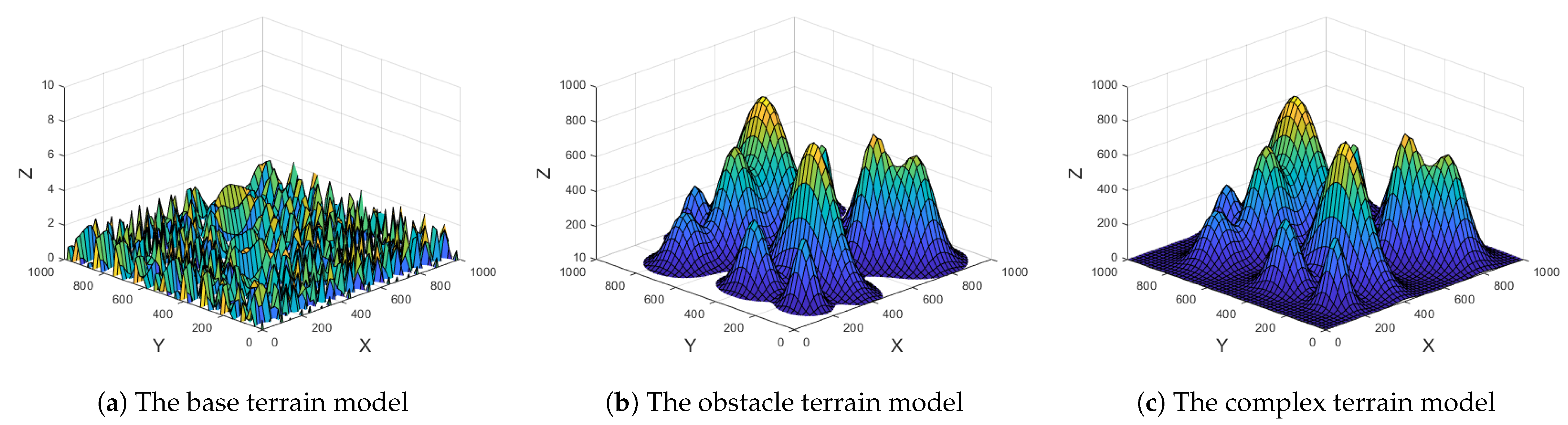
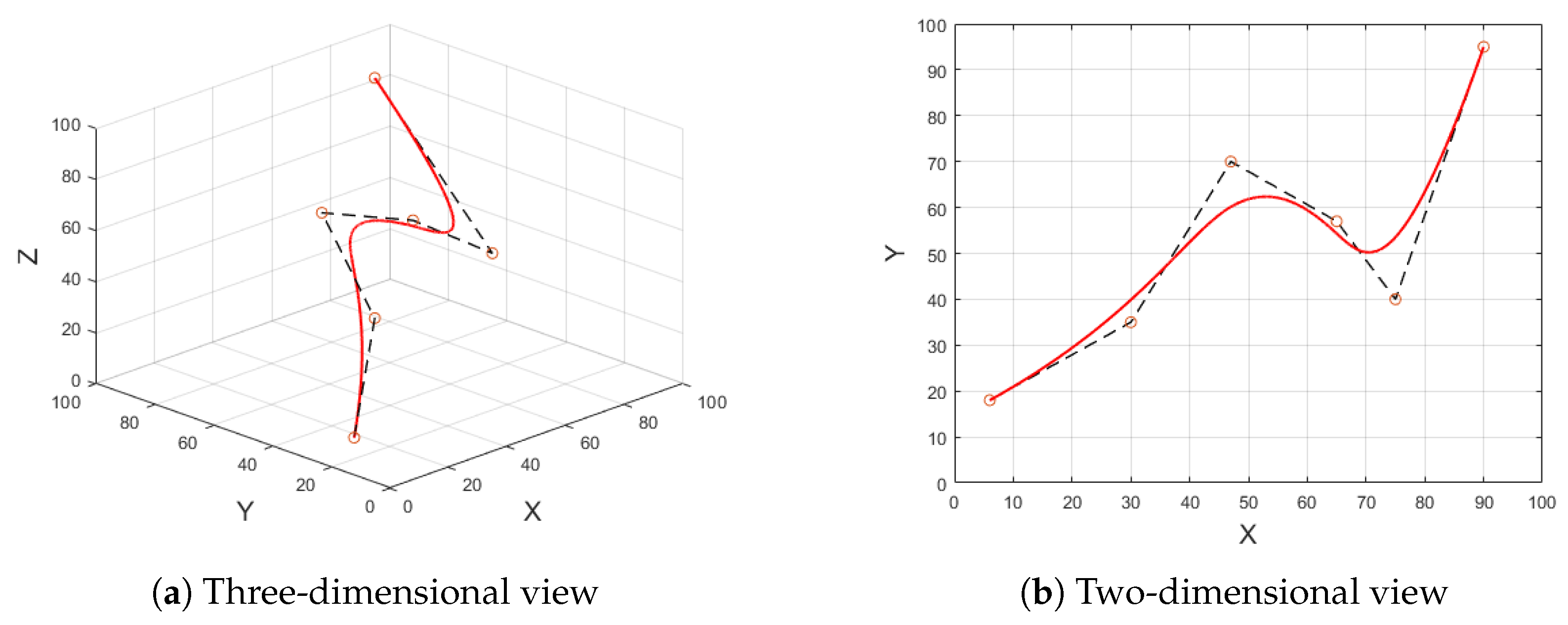
Furthermore, a three-dimensional complex terrain model with various obstacles is established, and the cubic B-spline curves are utilized to smooth the flight trajectory. The cost function considers five key factors: flight distance, flight height, flight turning angle, collisions between UAVs and obstacles, and collisions among multiple UAVs. To validate the optimization capabilities of AI-SMA, the algorithm was tested against well-established meta-heuristics on the CEC 2017 benchmark test suite and various multi-UAV path-planning scenarios. The primary contributions of this study are summarized as follows:

• The multi-UAV path-planning problem is modeled as a constrained optimization problem, with the cost function including five key constraints. A complex terrain model is established to address multi-UAV path-planning challenges.
• A self-adaptive improved slime mold algorithm (AI-SMA) is introduced. Three significant enhancements are incorporated into this algorithm: a novel search mechanism, a self-adaptive switch operator, and a self-adaptive perturbation strategy.
• The performance of AI-SMA is assessed through the CEC 2017 benchmark test set and multi-UAV path-planning scenarios. Effectiveness analysis, convergence behavior analysis, strategy validity, and parameter analysis are conducted.

The rest of this paper is structured as follows. Section 2 establishes the multi-UAV path-planning model and defines the cost function. Section 3 provides preliminary information for SMA and rank-DE. Section 4 introduces the mathematical model of AI-SMA. Section 5 discusses the experimental results and analysis of AI-SMA. Finally, Section 6 provides the conclusions of the study.

2. Problem Statement

This section first established a 3D complex terrain model for multi-UAV path-planning scenarios. Then, the UAV trajectory representation and smoothing method employed are described. Lastly, a cost function and the objectives of the multi-UAV path-planning problem are formulated.

2.1. Scenario Setting

To simulate the real terrain environment, a complex terrain model is created that incorporates both the base terrain model and the obstacle terrain model. The base terrain model is described as follows [53]:

$$\begin{array}{c}\hfill Z_1(x,y)=\sin (y+a)+b·\sin \left(x\right)+c·\cos (d·\sqrt{y^2+x^2})+\\ \hfill e·\cos \left(y\right)+f·\sin (f·\sqrt{y^2+x^2})+g·\cos \left(y\right)\end{array}$$

(1)

where $(x,y)$ represents the coordinates of a point on the horizontal plane. The coefficients $a,b,c,d,e,f,g$ are constant values that simulate different rough terrain surfaces. According to the common settings in the literature, the coefficients are assigned as follows: $a=3\pi ,b=\frac{1}{10},c=\frac{9}{10},d=\frac{1}{2},e=\frac{1}{2},f=\frac{1}{2},g=\frac{3}{10}$ [54,55].

The base terrain model mainly considers the relief of the terrain, while the obstacle terrain model is created to simulate various shapes of obstacle threats. The obstacle terrain model can be described using the following Equation [56]:

$$Z_2(x,y)=\sum _{n=1}^{N_{obs}}{H}_n·exp\left[-{\left(\frac{x-x_{c,n}}{x_{s,n}}\right)}^2-{\left(\frac{y-y_{c,n}}{y_{s,n}}\right)}^2\right]$$

(2)

where $N_{obs}$ represents the number of obstacles and $H_n$ denotes the peak height of the n-th obstacle. The parameters $x_{c,n}$ and $y_{c,n}$ represent the abscissa and ordinate of the centroid for the n-th obstacle, respectively. $x_{s,n}$ denotes the slope of the n-th obstacle along the X-axis, while $y_{s,n}$ denotes the slope along the Y-axis.

The different parameters in the two models above can collectively contribute to the diversity of obstacle scenarios. The complex terrain model is described as follows:

$$Z(x,y)=\max [Z_1(x,y),Z_2(x,y)]$$

(3)

where $Z_1(x,y)$ denotes the height of the base terrain model at $(x,y)$ and $Z_2(x,y)$ denotes the height of the obstacle terrain model at that point.

An example of the base terrain model, the obstacle terrain model, and the complex terrain model is shown in Figure 1a, Figure 1b, and Figure 1c, respectively.

2.2. Path Representation

In multi-UAV path planning, the flight trajectory of each UAV consists of a series of waypoints. Let M denote the number of UAVs and N denote the number of waypoints. For each UAV $m\in \{1,\dots ,M\}$, assuming that it flies from the starting point $P_s^m=(x_s^m,y_s^m,z_s^m)$ to the terminal point $P_t^m=(x_t^m,y_t^m,z_t^m)$ at the same speed. The flight trajectory of the UAV can be described as a discrete sequence of coordinates as follows:

$$W{P}^m=\{P_1^m,P_2^m,\dots ,P_{N-1}^m,P_N^m\},m=1,\dots ,M$$

(4)

where $P_i^m$ presents the i-th waypoint of the m-th UAV, with $P_1^m=P_s^m$ and $P_N^m=P_t^m$. Each waypoint $P_i^m$ can be expressed as follows:

$$P_i^m=\{x_i^m,y_i^m,z_i^m\},i=1,\dots ,N$$

(5)

where $x_i^m$, $y_i^m$, and $z_i^m$ represent the X-axis, Y-axis, and Z-axis coordinates in three-dimensional space, respectively.

The primary objective of multi-UAV path planning is to locate a set of waypoints $WP=\{W{P}^1,W{P}^2,\dots ,W{P}^M\}$ that minimizes the total cost of the flight trajectories.

However, the trajectory formed by connecting waypoints constitutes a continuous yet non-differentiable polyline, which fails to meet the practical requirements for UAV navigation. To resolve this limitation, a smoothing strategy is essential to ensure flight trajectories that are kinematically feasible and continuously differentiable.

Common methods for curve smoothing include Dubins curves [57], Savitzky–Golay filter [58], B-spline curves [59], etc. Among these, the B-spline curves method is particularly well-suited for UAV path smoothing because of its geometrical invariance, preservation of convexity, and affine invariance [60]. Moreover, a key advantage of the B-spline curves is that the polynomial degree remains constant even as the number of control points increases, significantly reducing the complexity of the path-smoothing process. A B-spline curve can be defined as follows:

$$P\left(t\right)=\sum _{i=0}^{N_{control}}{d}_i·N_{i,k}\left(t\right)$$

(6)

where $d_i(i=0,1,\dots ,N_{control})$ are control points, k is the order of the polynomial segments of the B-spline curves, and $N_{i,k}\left(t\right)$ are the k-order normalized B-spline blending functions described by a non-decreasing sequence of real numbers called knot sequence $\{t_0\le t_1\le \dots \le t_{n+k}\}$. The $N_{i.k}$ function is defined as follows:

$$\left\{\begin{array}{c}{N}_{i,1}\left(t\right)=\left\{\begin{array}{cc}1,\hfill & if{t}_i\le t\le t_{i+1}\hfill \\ 0,\hfill & otherwise\hfill \end{array}\right.\hfill \\ N_{i,k}\left(t\right)=\frac{t-t_i}{t_{i+k-1}-t_i}·N_{i,k-1}\left(t\right)+\frac{t_{i+k}-t}{t_{i+k}-t_{i+1}}·N_{i+1,k-1}\left(t\right)\hfill \end{array}\right.$$

(7)

This paper uses the cubic B-spline curves ($k=3$) to smooth the UAV flight trajectories because they can handle complex geometries with high precision and smoothness [61]. An example of the cubic B-Spline curves with six control points is shown in Figure 2a and Figure 2b, respectively.

2.3. Cost Function

The cost function for path planning is a mathematical model that balances various factors involved in the flight process and quantifies the constraints. It can be considered as the objective function in path-planning problems. By optimizing the cost function value, algorithms can efficiently locate the optimal solution within the specified search space. In this paper, the cost function considers five key factors: flight distance, flight height, flight turning angle, the collision between UAVs and obstacles, and the collision between multiple UAVs.

2.3.1. Flight Distance Cost

Time is of the essence when UAVs are on a mission. Less flight time will allow UAVs to reach the designated location faster and consume less energy. Minimizing the flight time is equivalent to minimizing the flight distance if UAVs fly at a constant speed. The flight distance of a UAV can be modeled as a sequence of line segments connected by waypoints in the following:

$$D^m=\{\parallel \overrightarrow{P_1^m{P}_2^m}\parallel ,\dots ,\parallel \overrightarrow{P_{N-1}^m{P}_N^m}\parallel \}$$

(8)

where $D^m$ denotes the collection of flight segments of the m-th UAV and $\parallel \overrightarrow{P_i{P}_j}\parallel$ denotes the Euclidean distances between waypoints $P_i$ and $P_j$.

The flight distance cost for the m-th UAV is calculated as the ratio of the total length of all waypoint connections of this UAV to the Euclidean distance between the starting and terminal points. This is mathematically expressed in the following:

$$C_{distance}^m=\frac{{\sum }_{n=1}^{N-1}\parallel \overrightarrow{P_n{P}_{n+1}}\parallel }{\parallel \overrightarrow{P_1{P}_N}\parallel }$$

(9)

2.3.2. Flight Height Cost

In addition to minimizing flight distance, limiting altitude variations is important for reducing energy consumption. Each UAV has to operate within defined upper and lower height boundaries during its tasks. If a UAV flies above the upper limit or below the lower limit, it will incur penalties. The flight height cost for the m-th UAV is formulated as the sum of the height penalties received during flight, as follows:

$$C_{height}^m=\sum _{i=2}^{N-1}{Q}_{height,i}^m$$

(10)

$$Q_{height,i}^m=\left\{\begin{array}{cc}{q}_{height},\hfill & if{z}_i^m<z_{lb}or{z}_i^m>z_{ub}\hfill \\ 0,\hfill & otherwise\hfill \end{array}\right.$$

(11)

where $Q_{height,i}^m$ denotes the flight height cost for the m-th UAV at the i-th waypoint. Notably, the starting and terminal points are excluded from the calculation to conserve computing resources. $z_i^m$ denotes the height of the m-th UAV at the i-th waypoint, while $z_{lb}$ and $z_{ub}$ represent the lower and upper height limitations for all UAVs, respectively. $q_{height}$ denotes the cost coefficient of the flight height cost.

2.3.3. Flight Turning Cost

The inherent maneuverability of UAVs restricts their turning to specific angle ranges. The yaw and pitch angles are critical for maintaining the orientation of UAVs in horizontal and vertical directions, respectively. The yaw angle determines the heading of UAVs in the horizontal plane, ensuring proper directional control towards the target. The pitch angle regulates the tilt of UAVs in the vertical plane, influencing altitude changes and its ability to climb or descend. An example of the yaw angle and pitch angle for the m-th UAV in the i-th waypoint are illustrated in Figure 3a and Figure 3b, respectively.

Any turning maneuver that surpasses these predefined angular thresholds is deemed kinematically infeasible and requires punishment. Therefore, restricting the yaw and pitch angle range during UAV flight is necessary. The flight turning cost for the m-th UAV is defined as the sum of yaw angle and pitch angle penalties during flight, as follows:

$$C_{turn}^m=\sum _{i=2}^{N-1}{Q}_{yaw,i}^m+\sum _{i=2}^{N-1}{Q}_{pitch,i}^m$$

(12)

$$Q_{yaw,i}^m=\left\{\begin{array}{cc}{q}_{yaw},\hfill & otherwise\hfill \\ 0,\hfill & if0\le {\alpha }_i^m\le {\alpha }_{max}\hfill \end{array}\right.$$

(13)

$$Q_{pitch,i}^m=\left\{\begin{array}{cc}{q}_{pitch},\hfill & otherwise\hfill \\ 0,\hfill & if0\le {\beta }_i^m\le {\beta }_{max}\hfill \end{array}\right.$$

(14)

where $Q_{pitch,i}^m$ and $Q_{pitch,i}^m$ represent the i-th yaw angle cost and the i-th pitch angle cost for the m-th UAV, respectively. The i-th yaw angle is denoted as ${\alpha }_i^m$ and the i-th pitch angle is represented as ${\beta }_i^m$. $q_{yaw}$ and $q_{pitch}$ denote the cost coefficients of the flight turning cost. The calculations for ${\alpha }_i^m$ and ${\beta }_i^m$ are specified as follows [62,63]:

$${\alpha }_i^m=arccos\frac{(x_i^m-x_{i-1}^m)·(x_{i+1}^m-x_i^m)+(y_i^m-y_{i-1}^m)·(y_{i+1}^m-y_i^m)}{\sqrt{{(x_i^m-x_{i-1}^m)}^2+{(y_i^m-y_{i-1}^m)}^2}·\sqrt{{(x_{i+1}^m-x_i^m)}^2+{(y_{i+1}^m-y_i^m)}^2}}$$

(15)

$${\beta }_i^m=arctan\frac{|Z_i^m-Z_{i-1}^m|}{\sqrt{{(x_i^m-x_{i-1}^m)}^2+{(y_i^m-y_{i-1}^m)}^2}}$$

(16)

2.3.4. Collision Cost Between UAVs and Obstacles

In the course of the mission, ensuring the safety of the UAV is of utmost importance. The collision cost between UAVs and obstacles such as mountains and rocks must be considered. If the UAV collides with an obstacle during flight, penalties must be imposed. The collision cost of the m-th UAV with obstacles is formulated as the total penalty incurred from collisions during flight, as follows:

$$C_{collision\_obs}^m=\sum _{i=1}^{N-1}{Q}_{collision\_obs,i}^m$$

(17)

$$Q_{collision\_obs,i}^m=\left\{\begin{array}{cc}{q}_{collision\_obs},\hfill & if(x_i^m,y_i^m,z_i^m)isinobstacles\hfill \\ 0,\hfill & otherwise\hfill \end{array}\right.$$

(18)

where $Q_{collision\_obs,i}^m$ denotes the collision cost for the m-th UAV with obstacles at the i-th waypoint and $q_{collision\_obs}$ denotes the cost coefficient.

2.3.5. Collision Cost Between UAVs

It is crucial to avoid collisions with obstacles and collisions between UAVs when multiple UAVs operate simultaneously. Collisions arise from overlapping flight trajectories or inadequate safety distance between UAVs, potentially leading to substantial losses and system failures. The collision cost between the m-th UAV and other UAVs is calculated as the total penalty incurred from collisions with other UAVs during flight, as follows:

$$C_{collision\_uav}^m=\sum _{i=2}^{N-1}\sum _{n=1,n\ne m}^M{Q}_{collision\_uav,i}^{m,n}$$

(19)

$$Q_{collision\_uav,i}^{m,n}=\left\{\begin{array}{cc}0,\hfill & if\parallel \overrightarrow{P_i^m{P}_i^n}\parallel >d_{min}\hfill \\ q_{collision\_uav},\hfill & otherwise\hfill \end{array}\right.$$

(20)

where $Q_{collision\_uav,i}^{m,n}$ and $\parallel \overrightarrow{P_i^m{P}_i^n}\parallel$ represent the collision cost and the Euclidean distances between the m-th UAV and the n-th UAV at the i-th waypoint. $d_{min}$ denotes the minimum safe distance between two UAVs. $q_{collision\_uav}$ denotes the cost coefficient.

2.3.6. Total Cost and Objective Function

The quality of UAV flight trajectories can be quantified by converting the five flight constraints above into cost functions. The multi-UAV path-planning problem in this study aims to enable multiple UAVs to fly from the designated starting point to the destination with minimal flight distances. During operation, UAVs should adhere to altitude and turning angle limitations while avoiding collisions with obstacles and other UAVs; otherwise, penalties will be received. Therefore, the proposed algorithm should determine the optimal flight trajectories for all UAVs by minimizing the total cost function $C_{total}$. The objective function is defined as follows:

$$min{C}_{total}=min\sum _{m=1}^M{\omega }_1·C_{distance}^m+{\omega }_2·C_{height}^m+{\omega }_3·C_{turn}^m+{\omega }_4·C_{collision\_obs}^m+{\omega }_5·C_{collision\_uav}^m$$

(21)

where ${\omega }_1,{\omega }_2,{\omega }_3,{\omega }_4,{\omega }_5$ are weight coefficients for each cost function.

3. Preliminary Knowledge

This section provides an overview of SMA, including detailed mathematical formulations and illustrative diagrams. Subsequently, the rank-DE integrated into AI-SMA is explained by dividing into three parts.

3.1. Slime Mold Algorithm

SMA is a meta-heuristic optimization algorithm inspired by the foraging behavior of Physarum polycephalum, a species of slime mold found in nature [47]. During foraging, the slime mold extends its front end into a fan-shaped structure, forming an interconnected vein network that facilitates cytoplasmic flow, enabling efficient food source localization [64]. The slime mold dynamically adjusts the width of its veins based on food concentration. In regions with high food concentration, propagation waves generated by its biological oscillator enhance cytoplasmic flow, thickening the veins to promote nutrient foraging. Conversely, veins thin or disappear in areas with low food concentration to minimize energy expenditure. This positive–negative feedback mechanism allows the slime mold to construct optimal paths connecting multiple food sources.

SMA mathematically models this behavior by abstracting the morphological changes. The formula for updating the locations of the slime mold is as follows:

$$X(t+1)=\left\{\begin{array}{cc}ran{d}_2·(UB-LB)+LB,\hfill & ran{d}_2<z\hfill \\ X_{best}\left(t\right)+vb·\left((W·X_A\left(t\right)-X_B\left(t\right)\right),\hfill & ran{d}_1<p\hfill \\ vc·X\left(t\right),\hfill & ran{d}_1\ge p\hfill \end{array}\right.$$

(22)

where t is the index of the current iteration. $X\left(t\right)$ and $X(t+1)$ represent slime mold positions in the current and the next iteration. $UB$ and $LB$ represent the upper and lower boundaries of the search space, respectively. $ran{d}_1$ and $ran{d}_2$ are random numbers within the interval $[0,1]$. z is a small constant, typically set at 0.03, indicating the percentage of individuals within the slime mold that find food randomly.

In the initial stage, the slime mold randomly explores the search space within defined bounds to locate food sources. In search processes, it exhibits approaching behavior by navigating toward food sources based on environmental odor concentration gradients. The approaching behavior can be expressed in the following:

$$X(t+1)=\left\{\begin{array}{cc}{X}_{best}\left(t\right)+vb·\left(W·X_A\left(t\right)-X_B\left(t\right)\right),\hfill & ran{d}_1<p\hfill \\ vc·X\left(t\right),\hfill & ran{d}_1\ge p\hfill \end{array}\right.$$

(23)

where $X_{best}\left(t\right)$ represent the optimal position reached so far. $X_A\left(t\right)$ and $X_B\left(t\right)$ denote two randomly chosen individuals from the entire population.

When the slime mold approaches a region with a high concentration, it wraps the food by constricting the tissue structure of its veins. The food concentration in contact with the veins influences the strength of the waves generated by the biological oscillator of the slime mold. Higher food concentrations result in stronger waves, accelerating cytoplasmic flow and leading to thicker veins surrounding the food. In such cases, the slime mold focuses on existing food sources. On the contrary, in regions with low food concentration, the slime mold abandons the area and explores other regions to search for better food sources. This behavior reflects the transition of the slime mold between exploration and exploitation. The framework of SMA is illustrated in Figure 4.

The parameter p controls the exploration–exploitation pattern and is defined as follows:

$$p=tanh|Fit\left(X_i\right)-Fi{t}_{best}|,i=1,2,\dots ,NP$$

(24)

where $NP$ denotes the population size of the slime mold. $Fit\left(X_i\right)$ represents the fitness value of the i-th individual, while $Fi{t}_{best}$ denotes the best fitness achieved across all iterations, in other words, the global optimal fitness.

The parameters $vb$ and $vc$ simulate the exploration and exploitation behavior of slime molds as they approach food. $vb$ is a random number in the interval $[-a,a]$, representing the degree of exploration by the slime mold. $vc$ decreases linearly from 1 to 0, indicating the exploitation of historical information by each individual. The parameter a is determined in the following:

$$a=\mathrm{arctanh}(-\left(\frac{\mathit{t}}{{\mathit{t}}_{\mathit{max}}}\right)+1)$$

(25)

where $t_{max}$ denotes the maximum number of iterations.

The weight of the slime mold, W, is expressed by the following formulas:

$$W\left(FitIndex\left(i\right)\right)=\left\{\begin{array}{cc}1+ran{d}_1·log\left(\frac{BF-Fit\left(X_i\right)}{BF-WF}+1\right),\hfill & condition\hfill \\ 1-ran{d}_1·log\left(\frac{BF-Fit\left(X_i\right)}{BF-WF}+1\right),\hfill & others\hfill \end{array}\right.$$

(26)

$$FitIndex=sort\left(Fit\right)$$

(27)

where $FitIndex$ denotes the sequence generated after ranking the fitness value of all slime molds. In the case of minimization, the sorting is performed in ascending order. $condition$ indicates that $Fit\left(X_i\right)$ ranks first half of the population. $BF$ and $WF$ represent the best and the worst fitness value in the current iteration, respectively.

In SMA, parameters W, $vb$, and $vc$ collectively regulate the foraging mechanism. In detail, W simulates the oscillation frequency of slime mold as it approaches food sources with varying concentrations. This enables the slime mold to reach high-quality food more quickly while slowing down its approach to lower-concentration food, thereby improving its efficiency in selecting optimal food sources. The parameter $vb$ oscillates randomly within the range $[-a,a]$ and gradually converges to 0 as the number of iterations increases, while $vc$ fluctuates within $[-1,1]$ and eventually approaches zero. These two parameters jointly model the food selection behavior of the slime mold and help the algorithm to balance exploration and exploitation.

3.2. Ranking-Based Differential Evolution

Rank-DE is an alternative to differential evolution (DE), which is a popular algorithm for addressing global continuous optimization problems [65]. Inspired by the natural phenomenon where parent organisms with more valuable traits are more likely to reproduce offspring, rank-DE introduces ranking-based mutation operators built upon the foundation of traditional DE [52].

3.2.1. Ranking Assignment

To fully utilize the information from high-quality individuals, rank-DE first sorts the population based on their fitness. Then, each individual is assigned a ranking. In a minimization problem, the best individual receives the highest ranking of $NP-1$, and the worst individual is assigned the lowest ranking of 0. The ranking assignment rule is defined as follows:

$$R_j=NP-j,j=1,2,\dots ,NP$$

(28)

where j refers to the ranking index generated after sorting all individuals.

3.2.2. Selection Probability

Subsequently, the selection probability for each individual is calculated based on their ranking, reflecting the likelihood that the individual will be selected. The best individual in the minimization problem will have the highest selection probability $\frac{NP-1}{NP}$, and the worst individual will have the lowest selection probability of 0. The formula of selection probability is shown in the following:

$$P_j=\frac{R_j}{NP},j=1,2,\dots ,NP$$

(29)

where $P_j$ denotes the probability that the individual ranked in the j-th position in the population will be selected.

3.2.3. Vector Selection

Selection probabilities determine the mutation operator in rank-DE. This paper utilizes the rank-DE with the “DE/rand/1” mutation strategy. The original “DE/rand/1” mutation strategy can be defined in the following:

$$V_i=X_{r_1}+F·(X_{r_2}-X_{r_3})$$

(30)

where $r_1$, $r_2$, $r_3$ are distinct integers randomly chosen from the population range $[1,NP]$. The scaling factor F is chosen within the range $[0,2]$. $X_i$ represents the current position of the i-th individual, while $V_i$ indicates the position after mutation.

The pseudo-code for the rank-DE vector selection with the “DE/rand/1” mutation strategy is depicted in Algorithm 1. In rank-DE with “DE/rand/1”, $X_{r_1}$ and $X_{r_2}$ are selected according to their probabilities. $X_{r_1}$ serves as the base vector, while $X_{r_2}$ acts as the terminal vector. Since each individual has an assigned selection probability, better individuals are associated with higher probabilities. As a result, during the vector selection step, individuals with greater selection probabilities are more likely to be chosen as the base vector or the terminal point. This design improves the exploration capabilities of rank-DE and makes it more likely to converge on high-quality solutions. $X_{r_3}$ is randomly drawn from the population to enhance the algorithm’s randomness and prevent stagnation.

Algorithm 1 Rank-DE vector selection with “DE/rand/1”

Input: Population size NP, Selection probability P, Target individual index i. Output: Selected individual indexes $r_1$, $r_2$, $r_3$. 1: $r_1\leftarrow$ randomly select from $[1,NP]$; 2: while  $rand(0,1)>P_{r_1}$  or  $r_1==i$  do 3:       $r_1\leftarrow$ randomly select from $[1,NP]$; 4: end while 5: $r_2\leftarrow$ randomly select from $[1,NP]$; 6: while  $rand(0,1)>P_{r_2}$  or  $r_2==r_1$  or  $r_2==i$  do 7:       $r_2\leftarrow$ randomly select from $[1,NP]$; 8: end while 9: $r_3\leftarrow$ randomly select from $[1,NP]$; 10: while  $r_3==r_2$  or  $r_3==r_1$  or  $r_3==i$  do 11:       $r_3\leftarrow$ randomly select from $[1,NP]$; 12: end while

Then, the crossover operator is used to combine the existing individual $X_i$ with the mutated individual $V_i$ as follows:

$$U_i={[U_1,\dots ,U_{Dim}]}^T$$

(31)

$$U_{i,Dim}=\left\{\begin{array}{cc}{V}_{i,Dim},\hfill & ifrand<Cror{D}_{rand}=Dim\hfill \\ X_{i,Dim},\hfill & otherwise\hfill \end{array}\right.$$

(32)

where $Dim$ refers to the problem dimension and $D_{rand}$ represents the random integer in the interval of $[1,Dim]$. $rand$ is the random value in the interval of $[0,1]$. $Cr$ denotes the crossover parameter.

An example of the crossover process for six dimensions is shown in Figure 5.

Finally, a greedy selection principle is employed to retain better individuals. If the fitness value of the new individual $U_i$ outperforms the current individual $X_i$, $U_i$ is kept. Otherwise, $X_i$ is preserved for the next generation.

4. Proposed Algorithm

This section provides detailed information about the proposed algorithm. The steps and advantages of three enhancements of AI-SMA, i.e., a novel search mechanism, a self-adaptive switch operator, and a self-adaptive perturbation strategy, are explained. Additionally, the analysis of the computational complexity is provided. The complete pseudo-code of the algorithm and the framework diagram addressing the multi-UAV path-planning problems are shown.

4.1. A Novel Search Mechanism

The exploration versus exploitation trade-off is a constant challenge for meta-heuristic algorithms during the search process [66]. During the exploration phase, individuals are encouraged to search the solution space extensively, increasing the likelihood of finding a globally optimal solution. However, excessive exploration may lead to poor or no algorithm convergence. The exploitation phase promotes searching in small steps near the current optimal area, which allows the population to converge more quickly. Too much exploitation can trap the algorithm in local optima, resulting in premature convergence.

According to the position updating formula for SMA presented in Equation (22), when $ran{d}_2<z$, the algorithm simulates exploration behavior by generating random positions. If $ran{d}_2\ge z$, the algorithm manages the exploitation range of slime molds by adjusting the values of $vb$ and $vc$. Nevertheless, this approach significantly restricts the exploration ability of slime molds. Numerous experiments indicate that the value of z is typically set at 0.03, which makes a low exploration probability for the algorithm to escape optima, particularly when the population becomes homogenized during the later stages of iterations.

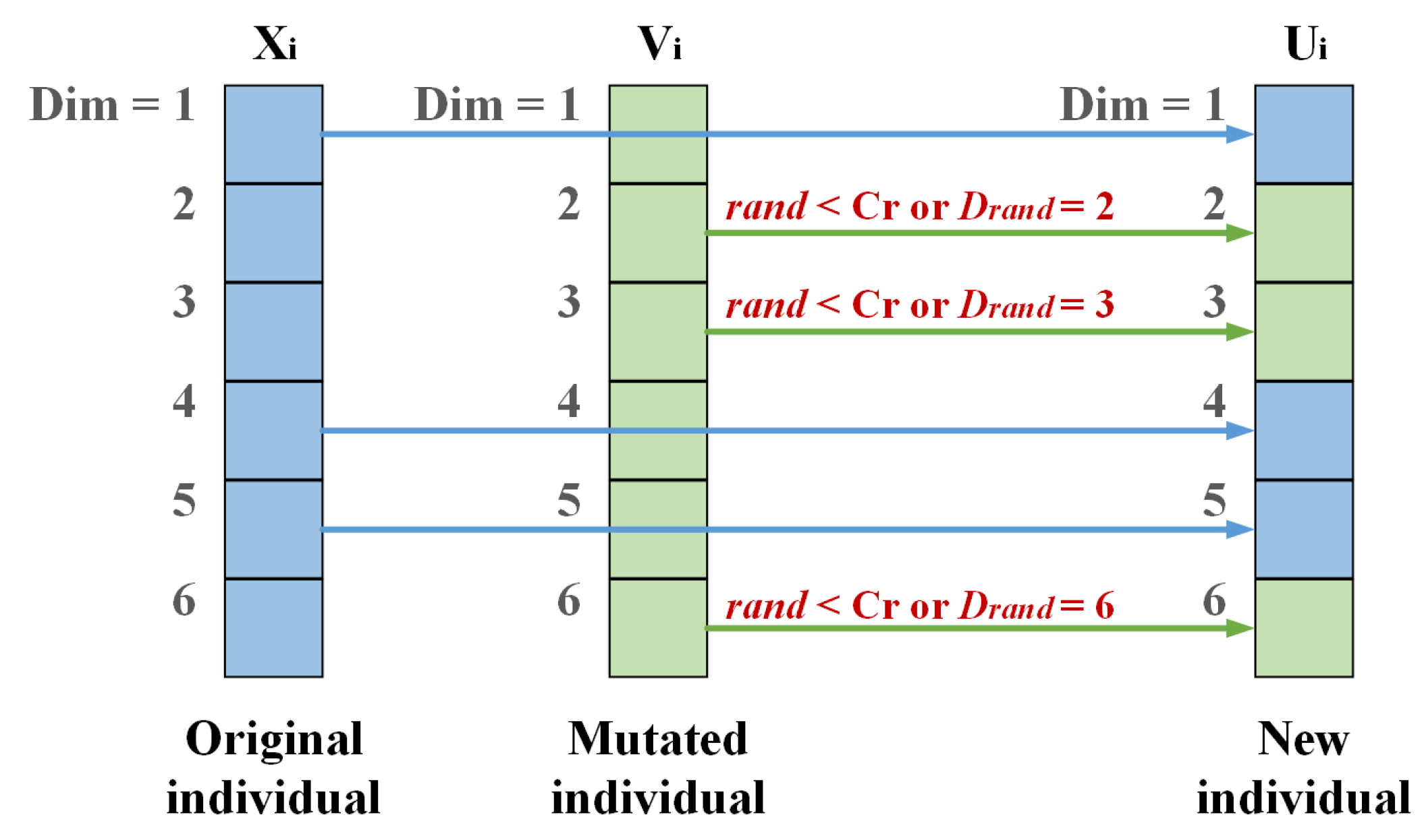
To this end, a novel search mechanism is proposed that replaces a portion of the exploitation phase in SMA with the mutation operation from rank-DE. The crossover operator $Cr$ replaces the parameter p, which controls the position update mode of slime molds. This integration of mutation and crossover from rank-DE increases the probability of the global search of SMA, effectively improving the exploration ability of AI-SNA and helping balance exploitation and exploration during the search process.

The novel position update formula is described as follows:

$$X_{new}\left(t\right)=\left\{\begin{array}{cc}ran{d}_2·(UB-LB)+LB,\hfill & ran{d}_2<S\hfill \\ X_{best}\left(t\right)+vb·\left(W·X_A\left(t\right)-X_B\left(t\right)\right),\hfill & ran{d}_1<Cr\hfill \\ X_{mutation}\left(t\right),\hfill & ran{d}_1\ge Cr\hfill \end{array}\right.$$

(33)

where $X_{new}\left(t\right)$ is the updated position resulting from the novel search mechanism in the current iteration. S denotes the self-adaptive switch operator, which will be discussed in Section 4.2. $X_{mutation}\left(t\right)$ represents the individual position after mutation, shown as follows:

$$X_{mutation}\left(t\right)=X_{r_1}\left(t\right)+2·ran{d}_3·vb·(X_{r_2}\left(t\right)-X_{r_3}\left(t\right))$$

(34)

The scaling factor F is replaced with a random value within the range $[0,2a]$ to avoid introducing new parameters into the algorithm. The individual indexes $r_1$, $r_2$, and $r_3$ are selected in Algorithm 1.

4.2. A Self-Adaptive Switch Operator

The optimization processes for most real-world problems exhibit non-linearity and complexity, which significantly constrain the performance of meta-heuristic algorithms with fixed search strategies. In SMA, the parameter z controls the behavior between local exploitation and global exploration. However, as iterations progress and population difference decreases, a fixed value for z may hinder the abilities of algorithms to explore better solutions.

Consequently, AI-S MA converts parameter z from a fixed probability into a non-linear parameter S. This transformation enables the algorithm to maintain a certain level of global search capability throughout the iterations, enhancing the quality of the optimal solution in the later stages and helping to prevent premature convergence.

The self-adaptive switch operator is calculated as follows:

$$S={log}_{10}(1+0.8·exp\left(\frac{t+1}{t_{max}}\right))$$

(35)

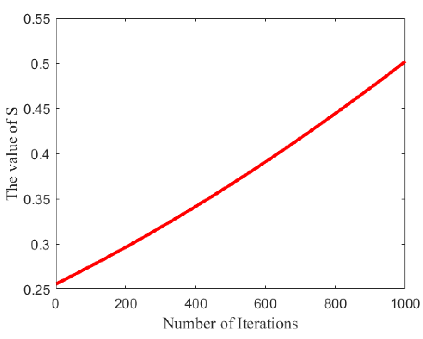
Figure 6 illustrates that the value of S grows as the iteration count increases. Initially, S is relatively small, indicating that the likelihood of the population generating random positions within the search space is minimal. This encourages individuals in the population to focus more on exploiting potential areas. As iterations progress, S gradually rises, which enhances the probability of random distribution among the individuals. This increase is beneficial for escaping the current optima and exploring promising regions throughout the optimization process.

In addition, considering the algorithm convergence, the growth range of S is intentionally limited. As shown in Figure 6, the value of S rises from approximately 0.2556 to 0.502 over 1000 iterations. This indicates that, in most cases, the population will effectively exploit the environment to locate the optimal solution, while the convergence curves will not oscillate due to the increased probability of randomness.

4.3. A Self-Adaptive Perturbation Strategy

When the population remains stagnant for several iterations, the positions of individuals tend to stabilize. This stability can lead to getting trapped in a local optimum, resulting in premature convergence. To address this issue, a self-adaptive perturbation strategy is implemented as a fine-tuning process within the population structure. This strategy aims to help the algorithm escape from suboptimal solutions when encountering stagnation.

In AI-SMA, a stagnation counter is initialized at zero to determine whether the algorithm has stagnated. In each iteration, the difference between the optimal fitness value of the current and previous iterations is calculated. In the first iteration, this difference is set to infinity. For subsequent iterations, if the absolute value of this difference is less than the perturbation operator, denoted as $\epsilon$, the stagnation counter is incremented by one. Otherwise, the counter is reset to zero. When the stagnation counter reaches the perturbation threshold, denoted as $N_{stag}$, the algorithm is considered stagnated, and the self-adaptive perturbation strategy is implemented. After applying the perturbation, the next iteration is executed. If the threshold has not been reached, AI-SMA proceeds directly to the next iteration. The algorithm terminates when the iteration count t reaches the maximum limitation $t_{max}$.

The core idea behind a self-adaptive perturbation strategy is to enhance the population by removing poorly performing individuals and replacing them with new ones. In detail, the worst-performing $\xi \times 100\%$ individuals are eliminated based on their fitness values. Subsequently, an additional $\xi \times 100\%$ new individuals are introduced to refresh the population. The positions of these newly added individuals are determined by balancing the optimal individual positions and randomly generated positions, ensuring that valuable information from the best individual is retained while incorporating some randomness.

The self-adaptive perturbation strategy is illustrated in the following:

$$X_{new}(t+1)=\left\{\begin{array}{cc}\lambda ·X_{best}\left(t\right)+(1-\lambda )·X_{rand}\left(t\right),\hfill & condition\hfill \\ X_{new}\left(t\right),\hfill & others\hfill \end{array}\right.$$

(36)

$$X_{rand}\left(t\right)=\mu ·(UB-LB)+LB$$

(37)

where $\lambda$ and $\mu$ are random number within the interval $[0,1]$. $X_{best}\left(t\right)$ represents the optimal position reached in all iterations. $condition$ indicates the worst $\xi$ individuals in the population, ranked by fitness value. $\epsilon$ is set to $1.00\times {10}^{-3}$ and $N_{stag}$ is set to 15 in this study.

Algorithm 2 presents the pseudo-code of AI-SMA.

Algorithm 2 The pseudo-code of AI-SMA

Input: Population size NP, Dimension Dim, Lower boundary LB, Upper Boundary UB, Maximum number of iterations $t_{max}$, Crossover Rate Cr, Perturbation Rate $\xi$. Output: Optimal position $X_{optimal}$, Optimal fitness $Fi{t}_{optimal}$. 1: Initialize the positions of population X and parameters; 2: $P\leftarrow$ calculate using Equation (29); 3: $N_{stag\_count}=0;t=1$; 4: while  $t\le t_{max}$  do 5:       $S\leftarrow$ calculate using Equation (35); 6:       $a\leftarrow$ calculate using Equation (25); 7:       for $i=1:NP$ do 8:             $Fit\left(X_i\right)\leftarrow$ calculate the fitness value for each $X_i$; 9:       end for 10:       $W\leftarrow$ calculate using Equation (26); 11:       $X_{best},Fi{t}_{best}\leftarrow$ evaluate the global optimal position and global optimal fitness; 12:       for $i=1:NP$ do 13:             if $ran{d}_2<S$ then 14:                 $X_{i,new}\leftarrow$ update the new position using Equation (33) (1); 15:             else 16:                 for $d=1:Dim$ do 17:                       if $ran{d}_1<Cr\mathbf{or}{D}_{rand}=Dim$ then 18:                             $X_{i,d,new}\leftarrow$ update the new position using Equation (33) (2); 19:                       else 20:                             $r_1,r_2,r_3\leftarrow$ select using Algorithm 1; 21:                             $X_{i,d,new}\leftarrow$ update the new position using Equation (33) (3); 22:                       end if 23:                 end for 24:             end if 25:             if $Fit\left(X_{i,new}\right)<Fit\left(X_i\right)$ then 26:                 Replace $X_i$ with $X_{i,new}$; 27:             end if 28:       end for 29:       $X_{best},Fi{t}_{best}\leftarrow$ update the global optimal position and global optimal fitness; 30:       if $|Fi{t}_{best}-Fi{t}_{best,t-1}|<\epsilon$ then 31:             $N_{stag\_count}=N_{stag\_count}+1$; 32:       else 33:             $N_{stag\_count}=0$; 34:       end if 35:       if $N_{stag\_count}\ge N_{stag}$ then 36:             $X_{new}(t+1)\leftarrow$ implement self-adaptive perturbation strategy using Equation (36); 37:       end if 38: end while

Overall, the framework of AI-SMA for addressing multi-UAV path-planning problems is depicted in Figure 7.

4.4. Computational Complexity Analysis

AI-SMA comprises six main components: initialization, selection probability calculation, fitness evaluation and sorting, weight matrix calculation, positions update, and self-adaptive perturbation strategy.

Let N be the population size, D the dimension of the problem, and T the maximum iteration limitation. The initialization process has a computational complexity of $O\left(D\right)$. The computation complexity for selection probability calculation is $O\left(N\right)$ [52]. These two processes are performed only once in AI-SMA and do not occur with iteration. In each iteration, the fitness evaluation and sorting require $O(N+NlogN)$, while the weight matrix calculation and positions updates both demand $O\left(ND\right)$. Although the perturbation strategy is not executed in every iteration, its worst-case computational complexity is $O\left(ND\right)$. Therefore, the overall computational complexity of AI-SMA is $O(D+N+T\times N\times (1+logN+D)$.

In comparison, the original SMA has a complexity of $O(D+T\times N\times (1+logN+D\left)\right)$ [47]. Though AI-SMA introduces an additional $O\left(N\right)$ complexity compared to SMA, its overall computational complexity remains roughly the same since $O\left(N\right)$ is dominated by $O\left(NlogN\right)$ for large values of N.

5. Simulation Results and Analysis

This section compares AI-SMA with seven well-known meta-heuristic algorithms using the CEC 2017 benchmark test suite. Following this comparison, experiments were conducted on multi-UAV path-planning problems using AI-SMA, conventional SMA, and three well-established SMA variants. Furthermore, parameter experiments were carried out to select the optimal parameter combinations. Strategy validity experiments were also undertaken to assess the effectiveness of different strategies within AI-SMA.

All experiments were performed on an Ubuntu 22.04.4 LTS operating system, equipped with 125 GiB of RAM and an Intel(R) Xeon(R) Gold 5218 GPU (2.30 GHz). The algorithms were implemented in Python 3.11.0, and the results were visualized using MATLAB R2022a.

5.1. CEC 2017 Experiments

The CEC 2017 benchmark test suite is widely recognized for evaluating real parameter single objective optimization problems [67]. Compared to the latest versions, such as CEC 2021 and CEC 2022, the CEC 2017 test suite offers a broader variety of functions, facilitating a more comprehensive evaluation across diverse scenarios [68,69]. It consists of 29 functions categorized into four groups: unimodal functions ($F_1,F_3$), simple multi-modal functions ($F_4–F_{10}$), hybrid functions ($F_{11}–F_{20}$), and composition functions ($F_{21}–F_{30}$). The definition domain for all functions is in the interval of $[-100,100]$. Details of benchmark functions are listed in

Table 1. Details of CEC 2017 benchmark functions.

Categories	Functions	${\mathit{Fit}}_{\mathit{min}}$
Unimodal Functions	$F_1\left(x\right)=$ Shifted and Rotated Bent Cigar Function	100
	$F_3\left(x\right)=$ Shifted and Rotated Zakharov Function	200
Simple Multi-modal Functions	$F_4\left(x\right)=$ Shifted and Rotated Rosenbrock’s Function	300
	$F_5\left(x\right)=$ Shifted and Rotated Rastrigin’s Function	400
	$F_6\left(x\right)=$ Shifted and Rotated Expanded Scaffer’s $F_7$ Function	500
	$F_7\left(x\right)=$ Shifted and Rotated Lunacek Bi-Rastrigin Function	600
	$F_8\left(x\right)=$ Shifted and Rotated Non-Continuous Rastrigin’s Function	700
	$F_9\left(x\right)=$ Shifted and Rotated Levy Function	800
	$F_{10}\left(x\right)=$ Shifted and Rotated Schwefel’s Function	900
Hybrid Functions	$F_{11}\left(x\right)=$ Hybrid Function 1 (N = 3)	1000
	$F_{12}\left(x\right)=$ Hybrid Function 2 (N = 3)	1100
	$F_{13}\left(x\right)=$ Hybrid Function 3 (N = 3)	1200
	$F_{14}\left(x\right)=$ Hybrid Function 4 (N = 4)	1300
	$F_{15}\left(x\right)=$ Hybrid Function 5 (N = 4)	1400
	$F_{16}\left(x\right)=$ Hybrid Function 6 (N = 4)	1500
	$F_{17}\left(x\right)=$ Hybrid Function 7 (N = 5)	1600
	$F_{18}\left(x\right)=$ Hybrid Function 8 (N = 5)	1700
	$F_{19}\left(x\right)=$ Hybrid Function 9 (N = 5)	1800
	$F_{20}\left(x\right)=$ Hybrid Function 10 (N = 6)	1900
Composition Functions	$F_{21}\left(x\right)=$ Composition Function 1 (N = 3)	2000
	$F_{22}\left(x\right)=$ Composition Function 2 (N = 3)	2100
	$F_{23}\left(x\right)=$ Composition Function 3 (N = 4)	2200
	$F_{24}\left(x\right)=$ Composition Function 4 (N = 4)	2300
	$F_{25}\left(x\right)=$ Composition Function 5 (N = 5)	2400
	$F_{26}\left(x\right)=$ Composition Function 6 (N = 5)	2500
	$F_{27}\left(x\right)=$ Composition Function 7 (N = 6)	2600
	$F_{28}\left(x\right)=$ Composition Function 8 (N = 6)	2700
	$F_{29}\left(x\right)=$ Composition Function 9 (N = 3)	2800
	$F_{30}\left(x\right)=$ Composition Function 10 (N = 3)	2900

, including the optimal fitness value ($Fi{t}_{min}$) for each function.

5.1.1. Effectiveness Analysis

To begin with, a numerical analysis was conducted using the CEC 2017 test set to verify the effectiveness of AI-SMA. AI-SMA was compared with seven well-regarded meta-heuristic algorithms, including SMA [47], DE [70], PSO [44], WOA [71], GWO [45], SSA [72], and SCA [73]. DE and PSO are the most influential and historically significant algorithms in the field [74,75]. WOA, GWO, SSA, and SCA are representative of popular meta-heuristic algorithms developed in recent years and have shown superior performance over other classic algorithms, such as GSA [76], GA [77], BA [78], and ACO [79], across multiple benchmark functions in their original literature. SMA, as the foundation of AI-SMA, was also included as a baseline for comparison.

The effectiveness of the algorithms was evaluated using three metrics: best fitness (BEST), average fitness (AVG), and standard deviation (STD). Best fitness indicates the best performance achieved by the algorithm, while average fitness determines the consistency of the optimal solution in multiple experiments. Standard deviation measures the stability of the algorithm. In general, a smaller value for each of these three metrics indicates better algorithm performance.

Furthermore, the Friedman test and Wilcoxon’s rank-sum test were employed to evaluate the overall performance of the algorithms and the significance of the results. The Friedman test is a non-parametric statistical approach that assesses the significance of differences in average algorithm rankings [80]. The algorithm that ranks first has the best overall performance. Wilcoxon’s test is utilized to ensure the superior performance of the algorithm is not due to random chance [81]. The performance of AI-SMA is considered justified if the test results are statistically significant.

The main parameter settings for these algorithms are outlined in

Table 2. The main parameter settings of algorithms for the CEC 2017 test set.

Algorithms	Parameter Settings
SMA [47]	$z=0.03$
DE [70]	$F=0.5,CR=0.5$
PSO [44]	$c_1=2,c_2=2,\omega =0.4$
WOA [71]	a is linearly decreased from 2 to 0, $b=1$
GWO [45]	a is linearly decreased from 2 to 0
SSA [72]	$c_2\in [0,1],c_3\in [0,1]$
SCA [73]	$a=2$
AI-SMA	$Cr=0.5,\xi =0.1$

. The parameters for AI-SMA were determined by parameter experiments in Section 5.4. The parameter configurations for other algorithms follow the recommended values from their original papers to ensure optimal performance. The population size ($NP$) and the problem dimension ($Dim$) are both set to 30, while the maximum iteration limitation ($t_{max}$) is configured to 1000. To reduce the impact of randomness, each algorithm was run 30 times independently.

The experimental outcomes of AI-SMA and its counterparts on the CEC 2017 benchmark functions are summarized in

Table 3. CEC 2017 experimental results with 30 Dim over 30 runs.

No.	Metrics	SMA	DE	PSO	WOA	GWO	SSA	SCA	AI-SMA
Unimodal Functions
$F_1$	BEST	$5.61\times {10}^4$	$2.88\times {10}^6$	$4.69\times {10}^{10}$	$3.08\times {10}^9$	$2.69\times {10}^7$	$3.26\times {10}^6$	$4.38\times {10}^8$	$\mathbf{7.71}\times {\mathbf{10}}^{\mathbf{2}}$
	AVG	$\mathbf{4.85}\times {\mathbf{10}}^{\mathbf{4}}$	$8.18\times {10}^6$	$3.06\times {10}^{10}$	$5.29\times {10}^9$	$3.84\times {10}^8$	$3.58\times {10}^8$	$4.51\times {10}^8$	$5.13\times {10}^4$
	STD	$\mathbf{5.46}\times {\mathbf{10}}^{\mathbf{4}}$	$1.17\times {10}^7$	$3.11\times {10}^{10}$	$6.37\times {10}^9$	$7.54\times {10}^8$	$2.54\times {10}^9$	$5.06\times {10}^8$	$1.22\times {10}^5$
$F_3$	BEST *	$2.00\times {10}^2$	$4.64\times {10}^2$	$4.87\times {10}^4$	$2.15\times {10}^4$	$3.18\times {10}^2$	$1.34\times {10}^3$	$7.54\times {10}^3$	$\mathbf{2.00}\times {\mathbf{10}}^{\mathbf{2}}$
	AVG	$\mathbf{1.08}\times {\mathbf{10}}^{\mathbf{2}}$	$1.04\times {10}^3$	$4.69\times {10}^4$	$1.92\times {10}^4$	$1.99\times {10}^3$	$9.24\times {10}^3$	$4.89\times {10}^3$	$1.26\times {10}^2$
	STD	$\mathbf{9.34}\times {\mathbf{10}}^{\mathbf{1}}$	$1.33\times {10}^3$	$4.83\times {10}^4$	$2.00\times {10}^4$	$3.52\times {10}^3$	$2.20\times {10}^4$	$5.06\times {10}^3$	$1.31\times {10}^2$
Simple Multi-modal Functions
$F_4$	BEST	$3.32\times {10}^2$	$3.32\times {10}^2$	$9.18\times {10}^3$	$6.75\times {10}^2$	$3.50\times {10}^2$	$4.51\times {10}^2$	$4.61\times {10}^2$	$\mathbf{3.21}\times {\mathbf{10}}^{\mathbf{2}}$
	AVG	$1.80\times {10}^2$	$\mathbf{1.77}\times {\mathbf{10}}^{\mathbf{2}}$	$6.96\times {10}^3$	$5.92\times {10}^2$	$2.48\times {10}^2$	$1.16\times {10}^3$	$2.67\times {10}^2$	$1.86\times {10}^2$
	STD	$1.66\times {10}^2$	$\mathbf{1.63}\times {\mathbf{10}}^{\mathbf{2}}$	$7.22\times {10}^3$	$6.51\times {10}^2$	$2.49\times {10}^2$	$2.67\times {10}^3$	$2.53\times {10}^2$	$1.74\times {10}^2$
$F_5$	BEST	$5.19\times {10}^2$	$6.65\times {10}^2$	$4.68\times {10}^4$	$1.27\times {10}^4$	$7.42\times {10}^2$	$6.51\times {10}^3$	$1.12\times {10}^3$	$\mathbf{4.59}\times {\mathbf{10}}^{\mathbf{2}}$
	AVG	$2.96\times {10}^2$	$3.54\times {10}^2$	$3.69\times {10}^4$	$1.24\times {10}^4$	$8.84\times {10}^2$	$5.76\times {10}^3$	$8.78\times {10}^2$	$\mathbf{2.62}\times {\mathbf{10}}^{\mathbf{2}}$
	STD	$2.83\times {10}^2$	$3.40\times {10}^2$	$3.78\times {10}^4$	$1.32\times {10}^4$	$1.26\times {10}^3$	$6.18\times {10}^3$	$9.08\times {10}^2$	$\mathbf{2.49}\times {\mathbf{10}}^{\mathbf{2}}$
$F_6$	BEST *	$5.00\times {10}^2$	$5.00\times {10}^2$	$5.00\times {10}^2$	$5.00\times {10}^2$	$5.00\times {10}^2$	$5.00\times {10}^2$	$5.00\times {10}^2$	$\mathbf{5.00}\times {\mathbf{10}}^{\mathbf{2}}$
	AVG *	$2.57\times {10}^2$	$2.57\times {10}^2$	$2.57\times {10}^2$	$2.57\times {10}^2$	$2.57\times {10}^2$	$2.57\times {10}^2$	$2.57\times {10}^2$	$\mathbf{2.57}\times {\mathbf{10}}^{\mathbf{2}}$
	STD *	$2.43\times {10}^2$	$2.43\times {10}^2$	$2.43\times {10}^2$	$2.43\times {10}^2$	$2.43\times {10}^2$	$2.43\times {10}^2$	$2.43\times {10}^2$	$\mathbf{2.43}\times {\mathbf{10}}^{\mathbf{2}}$
$F_7$	BEST	$8.36\times {10}^2$	$9.99\times {10}^2$	$1.59\times {10}^6$	$1.34\times {10}^5$	$4.35\times {10}^3$	$1.32\times {10}^4$	$2.43\times {10}^4$	$\mathbf{6.96}\times {\mathbf{10}}^{\mathbf{2}}$
	AVG	$4.64\times {10}^2$	$6.68\times {10}^2$	$1.22\times {10}^6$	$2.02\times {10}^5$	$1.91\times {10}^4$	$3.15\times {10}^4$	$1.82\times {10}^4$	$\mathbf{3.93}\times {\mathbf{10}}^{\mathbf{2}}$
	STD	$4.51\times {10}^2$	$6.92\times {10}^2$	$1.24\times {10}^6$	$2.28\times {10}^5$	$4.22\times {10}^4$	$1.47\times {10}^5$	$1.92\times {10}^4$	$\mathbf{3.80}\times {\mathbf{10}}^{\mathbf{2}}$
$F_8$	BEST	$8.36\times {10}^2$	$1.06\times {10}^3$	$1.35\times {10}^3$	$1.18\times {10}^3$	$\mathbf{7.90}\times {\mathbf{10}}^{\mathbf{2}}$	$1.35\times {10}^3$	$9.23\times {10}^2$	$8.10\times {10}^2$
	AVG	$5.04\times {10}^2$	$5.86\times {10}^2$	$7.55\times {10}^2$	$7.55\times {10}^2$	$4.66\times {10}^2$	$7.74\times {10}^2$	$5.06\times {10}^2$	$\mathbf{4.54}\times {\mathbf{10}}^{\mathbf{2}}$
	STD	$4.93\times {10}^2$	$5.72\times {10}^2$	$7.42\times {10}^2$	$7.46\times {10}^2$	$4.60\times {10}^2$	$7.61\times {10}^2$	$4.93\times {10}^2$	$\mathbf{4.41}\times {\mathbf{10}}^{\mathbf{2}}$
$F_9$	BEST *	$8.01\times {10}^2$	$8.00\times {10}^2$	$8.28\times {10}^2$	$8.10\times {10}^2$	$8.00\times {10}^2$	$8.09\times {10}^2$	$8.01\times {10}^2$	$\mathbf{8.00}\times {\mathbf{10}}^{\mathbf{2}}$
	AVG *	$4.12\times {10}^2$	$\mathbf{4.08}\times {\mathbf{10}}^{\mathbf{2}}$	$4.30\times {10}^2$	$4.18\times {10}^2$	$4.08\times {10}^2$	$4.13\times {10}^2$	$4.08\times {10}^2$	$4.09\times {10}^2$
	STD	$3.97\times {10}^2$	$\mathbf{3.93}\times {\mathbf{10}}^{\mathbf{2}}$	$4.15\times {10}^2$	$4.04\times {10}^2$	$3.94\times {10}^2$	$3.99\times {10}^2$	$3.94\times {10}^2$	$3.95\times {10}^2$
$F_{10}$	BEST	$3.33\times {10}^3$	$5.59\times {10}^3$	$7.83\times {10}^3$	$4.56\times {10}^3$	$2.90\times {10}^3$	$4.21\times {10}^3$	$5.45\times {10}^3$	$\mathbf{2.80}\times {\mathbf{10}}^{\mathbf{3}}$
	AVG	$2.20\times {10}^3$	$3.93\times {10}^3$	$4.26\times {10}^3$	$3.32\times {10}^3$	$2.66\times {10}^3$	$3.97\times {10}^3$	$3.09\times {10}^3$	$\mathbf{2.05}\times {\mathbf{10}}^{\mathbf{3}}$
	STD	$2.23\times {10}^3$	$3.96\times {10}^3$	$4.25\times {10}^3$	$3.42\times {10}^3$	$3.01\times {10}^3$	$4.06\times {10}^3$	$3.09\times {10}^3$	$\mathbf{2.09}\times {\mathbf{10}}^{\mathbf{3}}$
Hybrid Functions
$F_{11}$	BEST	$1.66\times {10}^4$	$2.26\times {10}^4$	$4.29\times {10}^8$	$6.36\times {10}^4$	$6.16\times {10}^4$	$5.20\times {10}^4$	$5.62\times {10}^4$	$\mathbf{1.29}\times {\mathbf{10}}^{\mathbf{4}}$
	AVG	$\mathbf{2.48}\times {\mathbf{10}}^{\mathbf{4}}$	$2.80\times {10}^4$	$7.37\times {10}^8$	$3.89\times {10}^6$	$5.62\times {10}^4$	$5.46\times {10}^7$	$5.62\times {10}^4$	$5.05\times {10}^4$
	STD	$\mathbf{2.83}\times {\mathbf{10}}^{\mathbf{4}}$	$3.73\times {10}^4$	$8.74\times {10}^8$	$2.94\times {10}^7$	$6.15\times {10}^4$	$2.59\times {10}^8$	$6.02\times {10}^4$	$6.92\times {10}^4$
$F_{12}$	BEST	$\mathbf{5.57}\times {\mathbf{10}}^{\mathbf{4}}$	$3.31\times {10}^6$	$4.45\times {10}^9$	$1.30\times {10}^6$	$3.82\times {10}^6$	$5.80\times {10}^5$	$1.98\times {10}^7$	$1.98\times {10}^5$
	AVG	$\mathbf{3.52}\times {\mathbf{10}}^{\mathbf{5}}$	$4.69\times {10}^6$	$3.79\times {10}^9$	$1.93\times {10}^7$	$1.18\times {10}^7$	$7.32\times {10}^8$	$1.79\times {10}^7$	$2.13\times {10}^6$
	STD	$\mathbf{5.11}\times {\mathbf{10}}^{\mathbf{5}}$	$7.20\times {10}^6$	$3.93\times {10}^9$	$3.21\times {10}^7$	$1.63\times {10}^7$	$1.72\times {10}^9$	$1.89\times {10}^7$	$3.71\times {10}^6$
$F_{13}$	BEST	$3.38\times {10}^4$	$2.86\times {10}^4$	$3.81\times {10}^9$	$6.87\times {10}^5$	$3.31\times {10}^5$	$4.78\times {10}^4$	$6.33\times {10}^6$	$\mathbf{1.08}\times {\mathbf{10}}^{\mathbf{4}}$
	AVG	$\mathbf{6.38}\times {\mathbf{10}}^{\mathbf{4}}$	$1.08\times {10}^5$	$4.23\times {10}^9$	$3.99\times {10}^7$	$3.99\times {10}^6$	$3.11\times {10}^8$	$5.90\times {10}^6$	$1.74\times {10}^5$
	STD	$\mathbf{8.92}\times {\mathbf{10}}^{\mathbf{4}}$	$1.79\times {10}^5$	$4.45\times {10}^9$	$9.74\times {10}^7$	$1.03\times {10}^7$	$1.04\times {10}^9$	$6.98\times {10}^6$	$5.33\times {10}^5$
$F_{14}$	BEST	$7.00\times {10}^4$	$\mathbf{4.00}\times {\mathbf{10}}^{\mathbf{3}}$	$8.61\times {10}^5$	$1.64\times {10}^5$	$7.64\times {10}^4$	$1.56\times {10}^5$	$1.03\times {10}^5$	$3.33\times {10}^4$
	AVG	$1.30\times {10}^5$	$\mathbf{4.23}\times {\mathbf{10}}^{\mathbf{3}}$	$2.10\times {10}^6$	$7.64\times {10}^5$	$2.01\times {10}^5$	$1.77\times {10}^6$	$1.67\times {10}^5$	$1.59\times {10}^5$
	STD	$1.84\times {10}^5$	$\mathbf{5.22}\times {\mathbf{10}}^{\mathbf{3}}$	$2.70\times {10}^6$	$1.31\times {10}^6$	$3.75\times {10}^5$	$2.74\times {10}^6$	$2.22\times {10}^5$	$2.27\times {10}^5$
$F_{15}$	BEST	$6.53\times {10}^4$	$4.61\times {10}^4$	$1.07\times {10}^9$	$1.43\times {10}^5$	$9.42\times {10}^4$	$3.66\times {10}^4$	$4.32\times {10}^5$	$\mathbf{1.16}\times {\mathbf{10}}^{\mathbf{4}}$
	AVG	$\mathbf{5.98}\times {\mathbf{10}}^{\mathbf{4}}$	$7.51\times {10}^4$	$1.95\times {10}^9$	$1.03\times {10}^7$	$2.60\times {10}^5$	$6.71\times {10}^8$	$1.02\times {10}^6$	$6.05\times {10}^4$
	STD	$\mathbf{7.42}\times {\mathbf{10}}^{\mathbf{4}}$	$1.10\times {10}^5$	$2.12\times {10}^9$	$3.40\times {10}^7$	$5.27\times {10}^5$	$1.92\times {10}^9$	$1.27\times {10}^6$	$1.38\times {10}^5$
$F_{16}$	BEST	$\mathbf{1.52}\times {\mathbf{10}}^{\mathbf{3}}$	$1.53\times {10}^3$	$9.83\times {10}^7$	$1.18\times {10}^4$	$1.96\times {10}^4$	$3.01\times {10}^3$	$2.19\times {10}^4$	$3.08\times {10}^3$
	AVG	$2.35\times {10}^3$	$\mathbf{8.37}\times {\mathbf{10}}^{\mathbf{2}}$	$3.81\times {10}^8$	$1.24\times {10}^6$	$7.14\times {10}^5$	$8.78\times {10}^4$	$2.17\times {10}^5$	$3.11\times {10}^3$
	STD	$3.72\times {10}^3$	$\mathbf{8.28}\times {\mathbf{10}}^{\mathbf{2}}$	$5.82\times {10}^8$	$2.88\times {10}^6$	$1.33\times {10}^6$	$1.99\times {10}^5$	$5.21\times {10}^5$	$4.11\times {10}^3$
$F_{17}$	BEST	$2.16\times {10}^3$	$2.47\times {10}^3$	$1.89\times {10}^9$	$2.33\times {10}^4$	$1.44\times {10}^4$	$2.03\times {10}^4$	$1.87\times {10}^4$	$\mathbf{2.08}\times {\mathbf{10}}^{\mathbf{3}}$
	AVG	$1.59\times {10}^3$	$2.89\times {10}^3$	$8.41\times {10}^{11}$	$1.36\times {10}^8$	$2.74\times {10}^4$	$1.27\times {10}^{14}$	$1.97\times {10}^4$	$\mathbf{1.55}\times {\mathbf{10}}^{\mathbf{3}}$
	STD	$1.61\times {10}^3$	$3.56\times {10}^3$	$2.82\times {10}^{12}$	$1.04\times {10}^9$	$3.11\times {10}^4$	$8.41\times {10}^{14}$	$2.07\times {10}^4$	$\mathbf{1.57}\times {\mathbf{10}}^{\mathbf{3}}$
$F_{18}$	BEST	$5.99\times {10}^4$	$\mathbf{1.65}\times {\mathbf{10}}^{\mathbf{4}}$	$2.23\times {10}^6$	$5.13\times {10}^4$	$5.41\times {10}^4$	$4.80\times {10}^4$	$1.18\times {10}^5$	$2.89\times {10}^4$
	AVG	$5.78\times {10}^4$	$\mathbf{2.43}\times {\mathbf{10}}^{\mathbf{4}}$	$6.00\times {10}^6$	$1.19\times {10}^5$	$1.87\times {10}^5$	$2.65\times {10}^6$	$1.56\times {10}^5$	$8.37\times {10}^4$
	STD	$6.24\times {10}^4$	$\mathbf{3.07}\times {\mathbf{10}}^{\mathbf{4}}$	$7.96\times {10}^6$	$1.73\times {10}^5$	$2.65\times {10}^5$	$6.78\times {10}^6$	$1.86\times {10}^5$	$1.11\times {10}^5$
$F_{19}$	BEST	$9.89\times {10}^3$	$\mathbf{1.91}\times {\mathbf{10}}^{\mathbf{3}}$	$1.71\times {10}^{10}$	$6.96\times {10}^4$	$2.96\times {10}^4$	$1.42\times {10}^4$	$1.12\times {10}^6$	$8.14\times {10}^3$
	AVG	$2.50\times {10}^4$	$\mathbf{1.41}\times {\mathbf{10}}^{\mathbf{3}}$	$1.11\times {10}^{12}$	$4.07\times {10}^7$	$3.82\times {10}^7$	$7.57\times {10}^8$	$6.78\times {10}^6$	$3.69\times {10}^5$
	STD	$3.30\times {10}^4$	$\mathbf{1.53}\times {\mathbf{10}}^{\mathbf{3}}$	$2.55\times {10}^{12}$	$1.24\times {10}^8$	$1.17\times {10}^8$	$3.44\times {10}^9$	$1.15\times {10}^7$	$7.39\times {10}^5$
$F_{20}$	BEST	$\mathbf{1.95}\times {\mathbf{10}}^{\mathbf{3}}$	$2.02\times {10}^3$	$6.39\times {10}^3$	$6.00\times {10}^3$	$1.96\times {10}^3$	$6.58\times {10}^3$	$2.38\times {10}^3$	$2.01\times {10}^3$
	AVG	$\mathbf{1.15}\times {\mathbf{10}}^{\mathbf{3}}$	$1.27\times {10}^3$	$5.59\times {10}^3$	$6.01\times {10}^3$	$1.25\times {10}^3$	$8.15\times {10}^3$	$1.47\times {10}^3$	$1.28\times {10}^3$
	STD	$\mathbf{1.15}\times {\mathbf{10}}^{\mathbf{3}}$	$1.29\times {10}^3$	$5.70\times {10}^3$	$6.49\times {10}^3$	$1.26\times {10}^3$	$8.98\times {10}^3$	$1.47\times {10}^3$	$1.28\times {10}^3$
Composition Functions
$F_{21}$	BEST *	$2.11\times {10}^3$	$2.17\times {10}^3$	$1.51\times {10}^4$	$3.98\times {10}^3$	$2.38\times {10}^3$	$2.39\times {10}^3$	$2.83\times {10}^3$	$\mathbf{2.11}\times {\mathbf{10}}^{\mathbf{3}}$
	AVG *	$1.11\times {10}^3$	$1.33\times {10}^3$	$1.48\times {10}^4$	$8.22\times {10}^3$	$1.64\times {10}^3$	$8.63\times {10}^3$	$1.68\times {10}^3$	$\mathbf{1.11}\times {\mathbf{10}}^{\mathbf{3}}$
	STD *	$1.10\times {10}^3$	$1.35\times {10}^3$	$1.62\times {10}^4$	$1.03\times {10}^4$	$1.73\times {10}^3$	$1.24\times {10}^4$	$1.69\times {10}^3$	$\mathbf{1.10}\times {\mathbf{10}}^{\mathbf{3}}$
$F_{22}$	BEST	$2.26\times {10}^3$	$2.27\times {10}^3$	$2.95\times {10}^3$	$2.84\times {10}^3$	$\mathbf{2.24}\times {\mathbf{10}}^{\mathbf{3}}$	$2.51\times {10}^3$	$2.31\times {10}^3$	$2.26\times {10}^3$
	AVG *	$\mathbf{1.14}\times {\mathbf{10}}^{\mathbf{3}}$	$1.15\times {10}^3$	$1.91\times {10}^3$	$1.97\times {10}^3$	$1.15\times {10}^3$	$2.24\times {10}^3$	$1.18\times {10}^3$	$1.14\times {10}^3$
	STD *	$\mathbf{1.13}\times {\mathbf{10}}^{\mathbf{3}}$	$1.14\times {10}^3$	$1.91\times {10}^3$	$2.01\times {10}^3$	$1.14\times {10}^3$	$2.41\times {10}^3$	$1.16\times {10}^3$	$1.13\times {10}^3$
$F_{23}$	BEST	$2.44\times {10}^3$	$2.62\times {10}^3$	$3.29\times {10}^4$	$8.90\times {10}^3$	$2.76\times {10}^3$	$2.70\times {10}^3$	$3.73\times {10}^3$	$\mathbf{2.39}\times {\mathbf{10}}^{\mathbf{3}}$
	AVG	$1.25\times {10}^3$	$2.85\times {10}^3$	$2.69\times {10}^4$	$1.08\times {10}^4$	$2.51\times {10}^3$	$1.22\times {10}^4$	$3.03\times {10}^3$	$\mathbf{1.23}\times {\mathbf{10}}^{\mathbf{3}}$
	STD	$1.24\times {10}^3$	$3.80\times {10}^3$	$2.73\times {10}^4$	$1.27\times {10}^4$	$2.94\times {10}^3$	$1.79\times {10}^4$	$3.09\times {10}^3$	$\mathbf{1.22}\times {\mathbf{10}}^{\mathbf{3}}$
$F_{24}$	BEST	$\mathbf{2.42}\times {\mathbf{10}}^{\mathbf{3}}$	$2.62\times {10}^3$	$2.45\times {10}^4$	$5.44\times {10}^3$	$2.83\times {10}^3$	$2.66\times {10}^3$	$3.88\times {10}^3$	$2.50\times {10}^3$
	AVG	$1.29\times {10}^3$	$1.70\times {10}^3$	$1.68\times {10}^4$	$8.16\times {10}^3$	$2.14\times {10}^3$	$4.44\times {10}^3$	$2.27\times {10}^3$	$\mathbf{1.27}\times {\mathbf{10}}^{\mathbf{3}}$
	STD	$1.28\times {10}^3$	$2.00\times {10}^3$	$1.71\times {10}^4$	$9.55\times {10}^3$	$2.42\times {10}^3$	$7.36\times {10}^3$	$2.27\times {10}^3$	$\mathbf{1.26}\times {\mathbf{10}}^{\mathbf{3}}$
$F_{25}$	BEST	$2.82\times {10}^3$	$2.82\times {10}^3$	$6.30\times {10}^3$	$3.08\times {10}^3$	$2.84\times {10}^3$	$3.09\times {10}^3$	$2.90\times {10}^3$	$\mathbf{2.76}\times {\mathbf{10}}^{\mathbf{3}}$
	AVG	$1.42\times {10}^3$	$1.42\times {10}^3$	$4.08\times {10}^3$	$1.73\times {10}^3$	$1.46\times {10}^3$	$1.87\times {10}^3$	$1.49\times {10}^3$	$\mathbf{1.39}\times {\mathbf{10}}^{\mathbf{3}}$
	STD	$1.41\times {10}^3$	$1.41\times {10}^3$	$4.13\times {10}^3$	$1.72\times {10}^3$	$1.44\times {10}^3$	$1.92\times {10}^3$	$1.48\times {10}^3$	$\mathbf{1.38}\times {\mathbf{10}}^{\mathbf{3}}$
$F_{26}$	BEST	$3.33\times {10}^3$	$3.33\times {10}^3$	$5.65\times {10}^3$	$3.40\times {10}^3$	$3.34\times {10}^3$	$4.32\times {10}^3$	$3.40\times {10}^3$	$\mathbf{2.91}\times {\mathbf{10}}^{\mathbf{3}}$
	AVG	$1.69\times {10}^3$	$1.68\times {10}^3$	$4.01\times {10}^3$	$2.38\times {10}^3$	$1.71\times {10}^3$	$6.12\times {10}^3$	$1.77\times {10}^3$	$\mathbf{1.47}\times {\mathbf{10}}^{\mathbf{3}}$
	STD	$1.67\times {10}^3$	$1.67\times {10}^3$	$4.12\times {10}^3$	$2.68\times {10}^3$	$1.69\times {10}^3$	$7.43\times {10}^3$	$1.75\times {10}^3$	$\mathbf{1.45}\times {\mathbf{10}}^{\mathbf{3}}$
$F_{27}$	BEST *	$3.11\times {10}^3$	$\mathbf{3.10}\times {\mathbf{10}}^{\mathbf{3}}$	$3.50\times {10}^3$	$3.40\times {10}^3$	$3.11\times {10}^3$	$3.73\times {10}^3$	$3.22\times {10}^3$	$3.10\times {10}^3$
	AVG	$1.57\times {10}^3$	$1.57\times {10}^3$	$1.99\times {10}^3$	$1.94\times {10}^3$	$1.58\times {10}^3$	$2.16\times {10}^3$	$1.64\times {10}^3$	$\mathbf{1.56}\times {\mathbf{10}}^{\mathbf{3}}$
	STD	$1.56\times {10}^3$	$1.55\times {10}^3$	$1.98\times {10}^3$	$1.93\times {10}^3$	$1.56\times {10}^3$	$2.16\times {10}^3$	$1.63\times {10}^3$	$\mathbf{1.54}\times {\mathbf{10}}^{\mathbf{3}}$
$F_{28}$	BEST	$\mathbf{2.72}\times {\mathbf{10}}^{\mathbf{3}}$	$2.79\times {10}^3$	$4.58\times {10}^3$	$3.22\times {10}^3$	$3.00\times {10}^3$	$3.40\times {10}^3$	$3.03\times {10}^3$	$3.19\times {10}^3$
	AVG	$1.49\times {10}^3$	$\mathbf{1.48}\times {\mathbf{10}}^{\mathbf{3}}$	$2.82\times {10}^3$	$1.74\times {10}^3$	$1.59\times {10}^3$	$2.88\times {10}^3$	$1.60\times {10}^3$	$1.61\times {10}^3$
	STD	$1.48\times {10}^3$	$\mathbf{1.47}\times {\mathbf{10}}^{\mathbf{3}}$	$2.83\times {10}^3$	$1.75\times {10}^3$	$1.57\times {10}^3$	$3.24\times {10}^3$	$1.59\times {10}^3$	$1.59\times {10}^3$
$F_{29}$	BEST	$7.86\times {10}^3$	$1.61\times {10}^4$	$3.67\times {10}^9$	$2.69\times {10}^5$	$4.42\times {10}^4$	$2.29\times {10}^8$	$6.02\times {10}^5$	$\mathbf{3.51}\times {\mathbf{10}}^{\mathbf{3}}$
	AVG	$4.28\times {10}^4$	$5.25\times {10}^5$	$5.06\times {10}^{10}$	$1.75\times {10}^8$	$5.14\times {10}^6$	$3.43\times {10}^{12}$	$2.79\times {10}^7$	$\mathbf{2.20}\times {\mathbf{10}}^{\mathbf{3}}$
	STD	$8.25\times {10}^4$	$2.68\times {10}^6$	$1.02\times {10}^{11}$	$4.27\times {10}^8$	$1.23\times {10}^7$	$2.31\times {10}^{13}$	$5.75\times {10}^7$	$\mathbf{2.20}\times {\mathbf{10}}^{\mathbf{3}}$
$F_{30}$	BEST	$3.39\times {10}^4$	$1.55\times {10}^5$	$9.01\times {10}^9$	$4.79\times {10}^5$	$1.89\times {10}^5$	$3.67\times {10}^5$	$1.69\times {10}^6$	$\mathbf{3.19}\times {\mathbf{10}}^{\mathbf{3}}$
	AVG	$8.01\times {10}^4$	$4.83\times {10}^5$	$2.76\times {10}^{10}$	$9.32\times {10}^7$	$1.79\times {10}^7$	$9.97\times {10}^{10}$	$1.88\times {10}^7$	$\mathbf{6.33}\times {\mathbf{10}}^{\mathbf{4}}$
	STD	$\mathbf{1.17}\times {\mathbf{19}}^{\mathbf{5}}$	$1.27\times {10}^6$	$6.03\times {10}^{10}$	$2.45\times {10}^8$	$1.06\times {10}^8$	$7.25\times {10}^{11}$	$6.34\times {10}^7$	$1.84\times {10}^5$
Mean Rank		1.28	1.79	6.69	5.16	3.00	5.29	3.84	0.92
Rank		2	3	8	6	4	7	5	1

* The actual numerical values represented in scientific notation differ.

, with the best performance for each function highlighted in bold. The Friedman test results are displayed in the last two rows of Table 3, while the statistical outcomes from Wilcoxon’s rank-sum test are illustrated in

Table 4. Statistical results from Wilcoxon’s rank-sum test ($p\ge 0.05$) on the CEC 2017 test suite.

AI-SMA vs.	Test Statistic	p-Value	Significance (Y/N)
SMA	$0.97\times {10}^2$	$8.01\times {10}^{-3}$	Y
DE	$1.04\times {10}^2$	$1.29\times {10}^{-2}$	Y
PSO	$0.00\times {10}^2$	$3.73\times {10}^{-9}$	Y
WOA	$0.00\times {10}^2$	$3.73\times {10}^{-9}$	Y
GWO	$0.24\times {10}^2$	$4.58\times {10}^{-5}$	Y
SSA	$0.02\times {10}^2$	$4.72\times {10}^{-6}$	Y
SCA	$00.8\times {10}^2$	$9.31\times {10}^{-8}$	Y

.

As presented in Table 3, benchmark functions are divided into 4 categories. In the first category, each unimodal function has a single optimal solution, which is useful for evaluating the exploitation capabilities of algorithms. AI-SMA achieves the best fitness for $F_1$ and $F_3$, ranking second in average fitness and standard deviation within this category. This demonstrates that the strong exploitation capabilities of SMA, which are retained in AI-SMA, help it to perform well on unimodal functions. The novel search mechanism also enables AI-SMA to discover better solutions than SMA in these functions.

Simple multi-modal functions, from $F_4$ to $F_{10}$, which contain many local optima, are ideal for examining the exploration abilities of algorithms. Experimental results indicate that AI-SMA achieves the best performance on $F_5$, $F_6$, $F_7$, and $F_{10}$, mainly because it employs mutation and crossover operators from rank-DE to enhance its exploitation capabilities. Although DE obtains a better average fitness and standard deviation than AI-SMA in $F_4$ and $F_9$, AI-SMA shows far superior exploration capabilities overall compared to other algorithms.

$F_{11}$ to $F_{20}$ are hybrid functions that consist of linear combinations of unimodal and simple multi-modal functions. Compared to the first two categories, these functions present a greater challenge and are suitable for testing the balance between exploitation and exploration in algorithms. AI-SMA outperforms others on $F_{17}$ and achieves the best fitness on $F_{11}$, $F_{13}$, and $F_{15}$. Despite AI-SMA ranking third behind SMA and DE in this category, its ability to attain the best fitness in various functions highlights its strong capacity to balance exploitation and exploration.

Regarding composition functions from $F_{21}$ to $F_{30}$, these functions are composed of non-linear combinations drawn from the previous three categories. They are recognized as the most complex functions within the test suite and are well-suited for evaluating the comprehensive effectiveness of the algorithm. Among these ten benchmark functions, AI-SMA shows superior performance compared to its competitors on five functions: $F_{21}$, $F_{23}$, $F_{25}$, $F_{26}$, and $F_{29}$. It also achieves the best average fitness on $F_{24}$, $F_{27}$, and $F_{30}$. These results suggest that the novel search mechanism proposed by AI-SMA effectively aids the algorithm in finding optimal fitness in complex functions. Moreover, the self-adaptive switch operator and the self-adaptive perturbation strategy help escape local optima, thereby avoiding premature convergence.

In the last two rows of Table 3, the Friedman test results indicate that AI-SMA ranks first among all eight algorithms, followed by SMA and DE. This ranking suggests that the proposed AI-SMA performs best across all functions tested. Moreover, AI-SMA improves the quality of optimal fitness by approximately $7.83\%$, $8.43\%$, $76.00\%$, $60.10\%$, $41.51\%$, $47.77\%$, and $53.99\%$ for the respective competing algorithms. Table 4 presents a pairwise comparison of the averages of the best solutions obtained for each algorithm. The significance level is set at $5\%$. Since the p-values obtained from the test are below 0.05, the results are considered statistically significant for the CEC 2017 test set. This demonstrates that the performance of AI-SMA is statistically robust and not due to random chance. In other words, the optimized solutions achieved by AI-SMA result from a systematic and structured optimization process.

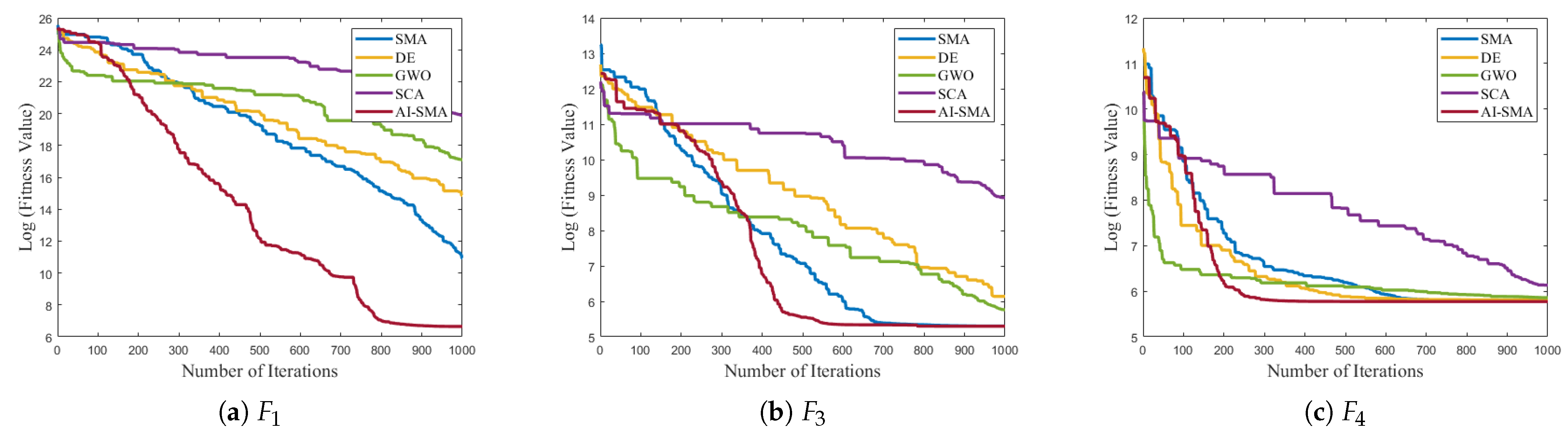
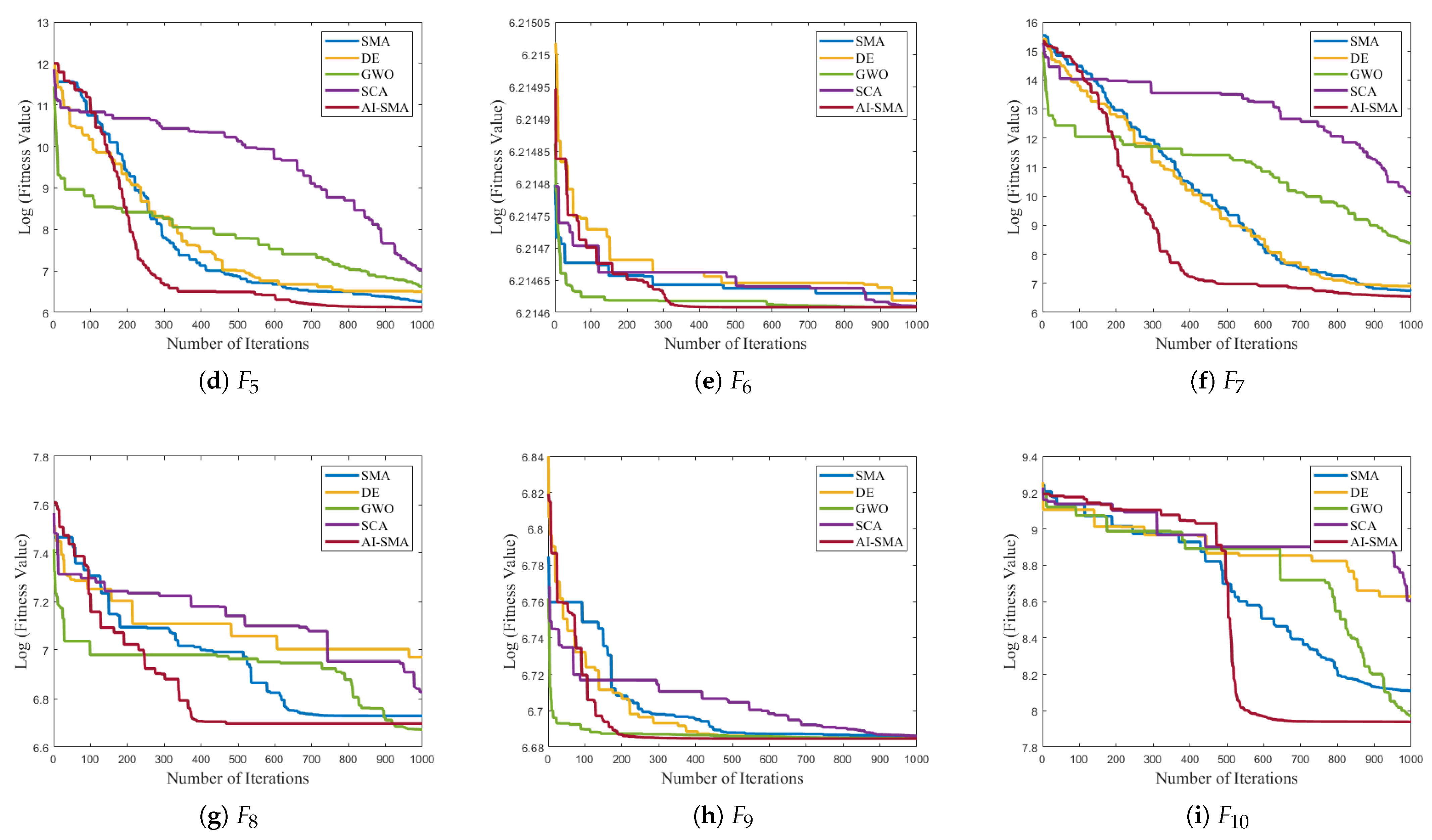
5.1.2. Convergence Behavior Analysis

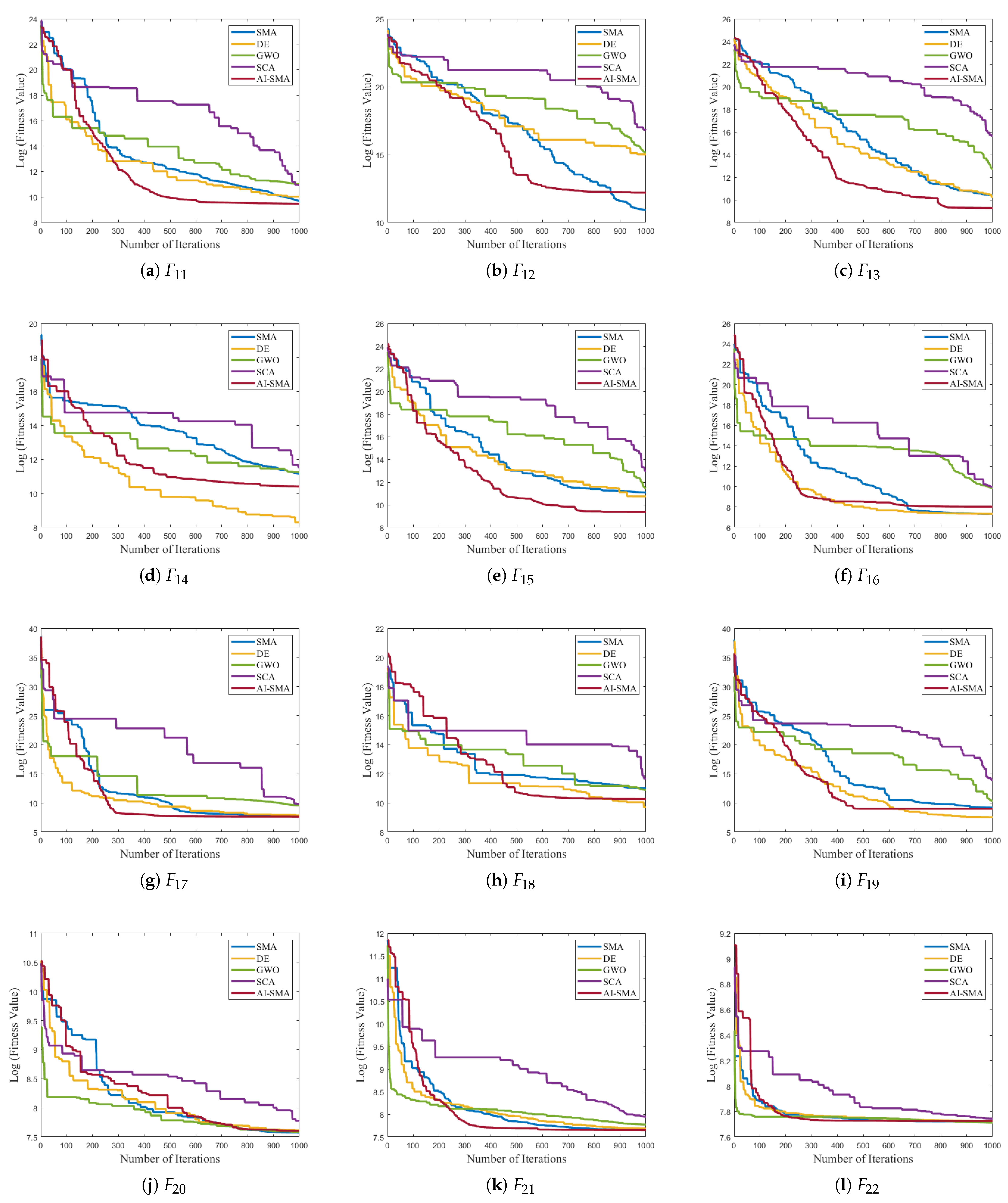
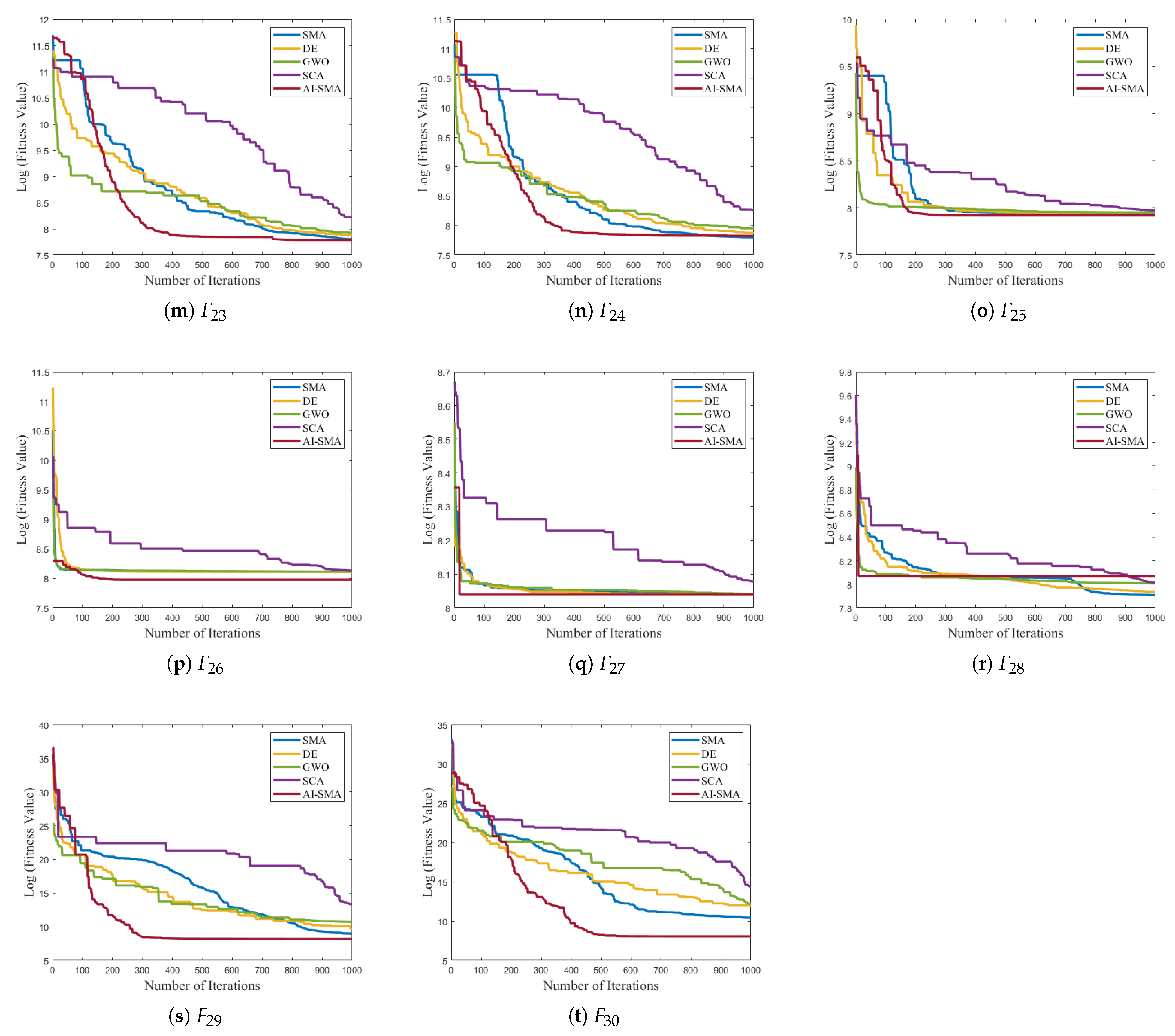
To further evaluate the convergence behavior of AI-SMA, the convergence curves of the top five well-performing algorithms in the effectiveness analysis were plotted. Figure 8 shows the convergence curves for benchmark functions $F_1$ to $F_{10}$, while the curves for $F_{11}$ to $F_{30}$ are presented in Figure A1 in Appendix A due to space limitations. The horizontal axis indicates the iteration count, and the vertical axis denotes the logarithm of the fitness value in these figures.

As depicted in Figure 8 and Figure A1, AI-SMA demonstrates stable convergence behavior across all functions, confirming the superior convergence properties. Additionally, AI-SMA converges more rapidly in the early stages than its competitors for most functions. This indicates that AI-SMA can detect stagnation and accelerate convergence through its self-adaptive perturbation strategy. Notably, AI-SMA exhibits superior convergence speed and the lowest fitness values than other algorithms on $F_1,F_7,F_{10},F_{13},F_{15},F_{29}$, and $F_{30}$. This swift convergence is particularly crucial in scenarios that require rapid computations, such as rescue operations and real-time optimization tasks.

5.2. Multi-UAV Path Planning

Multi-UAV path-planning problems are more complex than benchmark functions because of intricate constraints and non-linear cost functions. SMA and its variants, ESMA [82], CO-SMA [83], and SMA-AGDE [84], are selected as competitors for AI-SMA. These variants demonstrate excellent performance compared to common meta-heuristics discussed in their original papers. Among them, ESMA enhances SMA by integrating the Sine Cosine Algorithm (SCA), while CO-SMA offers a chaotic opposition-reinforced approach, combining the crossover-opposition technique with chaotic search methods. SMA-AGDE incorporates the adaptive guided differential evolution (AGDE) mutation method to improve the capabilities of SMA.

The test scenarios in this paper measure $1000\times 1000\times 1000$, with the number of UAVs and waypoints set to $M=5,N=10$. All UAVs are instructed to fly from the starting point (0, 0, 0) to the terminal point (1000, 1000, 0). The maximum yaw angle constraint ${\alpha }_{max}$ and the maximum pitch angle constraint ${\beta }_{max}$ are both set to ${45}^{°}$. The lower and upper height limitations for UAVs, $z_{lb}$ and $z_{ub}$, are set at 10 and 950, respectively. The minimum safe distance between UAVs is $d_{min}=5$. The cost coefficients for the cost function are set as follows: $q_{height}=100,q_{yaw}=100,q_{pitch}=100,q_{collision\_obs}=100,q_{collision\_uav}=100$. Additionally, the weight coefficients are assigned as ${\omega }_1=100,{\omega }_2=1,{\omega }_3=2,{\omega }_4=3,{\omega }_5=3$. Furthermore, the population size (NP) is fixed at 30, and the problem dimension ($Dim$) is fixed at 3. The maximum iteration limitation ($t_{max}$) is configured to 500. The results are based on 30 independent runs to ensure fairness. Details of the three scenarios are provided in

Table 5. Details of scenarios for multi-UAV path-planning problems.

Scenario 1
No.	Center Coordinate $({\mathit{x}}_{\mathit{c}},{\mathit{y}}_{\mathit{c}})$,	No.	Center Coordinate $({\mathit{x}}_{\mathit{c}},{\mathit{y}}_{\mathit{c}})$,
	Slope $({\mathit{x}}_{\mathit{sl}},{\mathit{y}}_{\mathit{sl}})$, and Height ${\mathit{h}}_{\mathit{m}}$		Slope $({\mathit{x}}_{\mathit{sl}},{\mathit{y}}_{\mathit{sl}})$, and Height ${\mathit{h}}_{\mathit{m}}$
1	(260, 210), (120, 115), 510	2	(430, 810), (100, 150), 750
3	(730, 350), (160, 150), 610
Scenario 2
No.	Center Coordinate $({\mathit{x}}_{\mathit{c}},{\mathit{y}}_{\mathit{c}})$,	No.	Center Coordinate $({\mathit{x}}_{\mathit{c}},{\mathit{y}}_{\mathit{c}})$,
	Slope $({\mathit{x}}_{\mathit{sl}},{\mathit{y}}_{\mathit{sl}})$, and Height ${\mathit{h}}_{\mathit{m}}$		Slope $({\mathit{x}}_{\mathit{sl}},{\mathit{y}}_{\mathit{sl}})$, and Height ${\mathit{h}}_{\mathit{m}}$
1	(210, 340), (110, 120), 410	2	(440, 710), (100, 150), 790
3	(200, 730), (110, 120), 390	4	(720, 810), (100, 150), 510
5	(800, 210), (100, 90), 330	6	(580, 220), (110, 120), 550
Scenario 3
No.	Center Coordinate $({\mathit{x}}_{\mathit{c}},{\mathit{y}}_{\mathit{c}})$,	No.	Center Coordinate $({\mathit{x}}_{\mathit{c}},{\mathit{y}}_{\mathit{c}})$,
	Slope $({\mathit{x}}_{\mathit{sl}},{\mathit{y}}_{\mathit{sl}})$, and Height ${\mathit{h}}_{\mathit{m}}$		Slope $({\mathit{x}}_{\mathit{sl}},{\mathit{y}}_{\mathit{sl}})$, and Height ${\mathit{h}}_{\mathit{m}}$
1	(160, 670), (78, 75), 390	2	(470, 280), (120, 105), 540
3	(750, 90), (90, 60), 430	4	(200, 750), (80, 80), 270
5	(400, 700), (90, 90), 500	6	(720, 720), (100, 170), 710
7	(950, 350), (55, 86), 400	8	(400, 900), (60, 60), 300
9	(850, 900), (70, 80), 500	10	(300, 120), (60, 70), 360

.

The parameter configurations for tested algorithms are provided in

Table 6. The parameter settings of algorithms for multi-UAV path-planning problems.

Algorithms	Parameter Settings
SMA [47]	$z=0.03$
ESMA [82]	$z=0.03,r_2\in [0,2\pi ]r_3\in [0,2]$
CO-SMA [83]	$z=0.03,{\beta }_0\in [0,1]$
SMA-AGDE [84]	$C{R}_1\in [0.05,0.15],C{R}_2\in [0.9,1.0]$
AI-SMA	$Cr=0.5,\xi =0.1$

. The parameters of competing algorithms align with the original literature.

Table 7. Multi-UAV path-planning problem results over 30 runs.

No.	Metrics	SMA	ESMA	CO-SMA	SMA-AGDE	AI-SMA
Scenario 1	BEST	$3.09\times {10}^3$	$\mathbf{2.29}\times {\mathbf{10}}^{\mathbf{3}}$	$2.31\times {10}^3$	$4.12\times {10}^3$	$3.94\times {10}^3$
	AVG	$7.92\times {10}^3$	$5.44\times {10}^3$	$\mathbf{4.01}\times {\mathbf{10}}^{\mathbf{3}}$	$5.32\times {10}^3$	$4.97\times {10}^3$
	STD	$1.84\times {10}^3$	$1.36\times {10}^3$	$9.97\times {10}^2$	$6.56\times {10}^2$	$\mathbf{4.75}\times {\mathbf{10}}^{\mathbf{2}}$
Scenario 2	BEST	$2.49\times {10}^3$	$3.48\times {10}^3$	$\mathbf{1.97}\times {\mathbf{10}}^{\mathbf{3}}$	$4.60\times {10}^3$	$3.84\times {10}^3$
	AVG	$8.70\times {10}^3$	$7.79\times {10}^3$	$5.87\times {10}^3$	$5.60\times {10}^3$	$\mathbf{4.84}\times {\mathbf{10}}^{\mathbf{3}}$
	STD	$2.03\times {10}^3$	$2.17\times {10}^3$	$1.95\times {10}^3$	$5.94\times {10}^2$	$\mathbf{4.80}\times {\mathbf{10}}^{\mathbf{2}}$
Scenario 3	BEST	$3.58\times {10}^3$	$2.77\times {10}^3$	$\mathbf{2.27}\times {\mathbf{10}}^{\mathbf{3}}$	$4.10\times {10}^3$	$3.12\times {10}^3$
	AVG	$7.79\times {10}^3$	$5.66\times {10}^3$	$\mathbf{3.77}\times {\mathbf{10}}^{\mathbf{3}}$	$5.45\times {10}^3$	$4.73\times {10}^3$
	STD	$1.59\times {10}^3$	$1.54\times {10}^3$	$1.05\times {10}^3$	$6.87\times {10}^2$	$\mathbf{5.44}\times {\mathbf{10}}^{\mathbf{2}}$

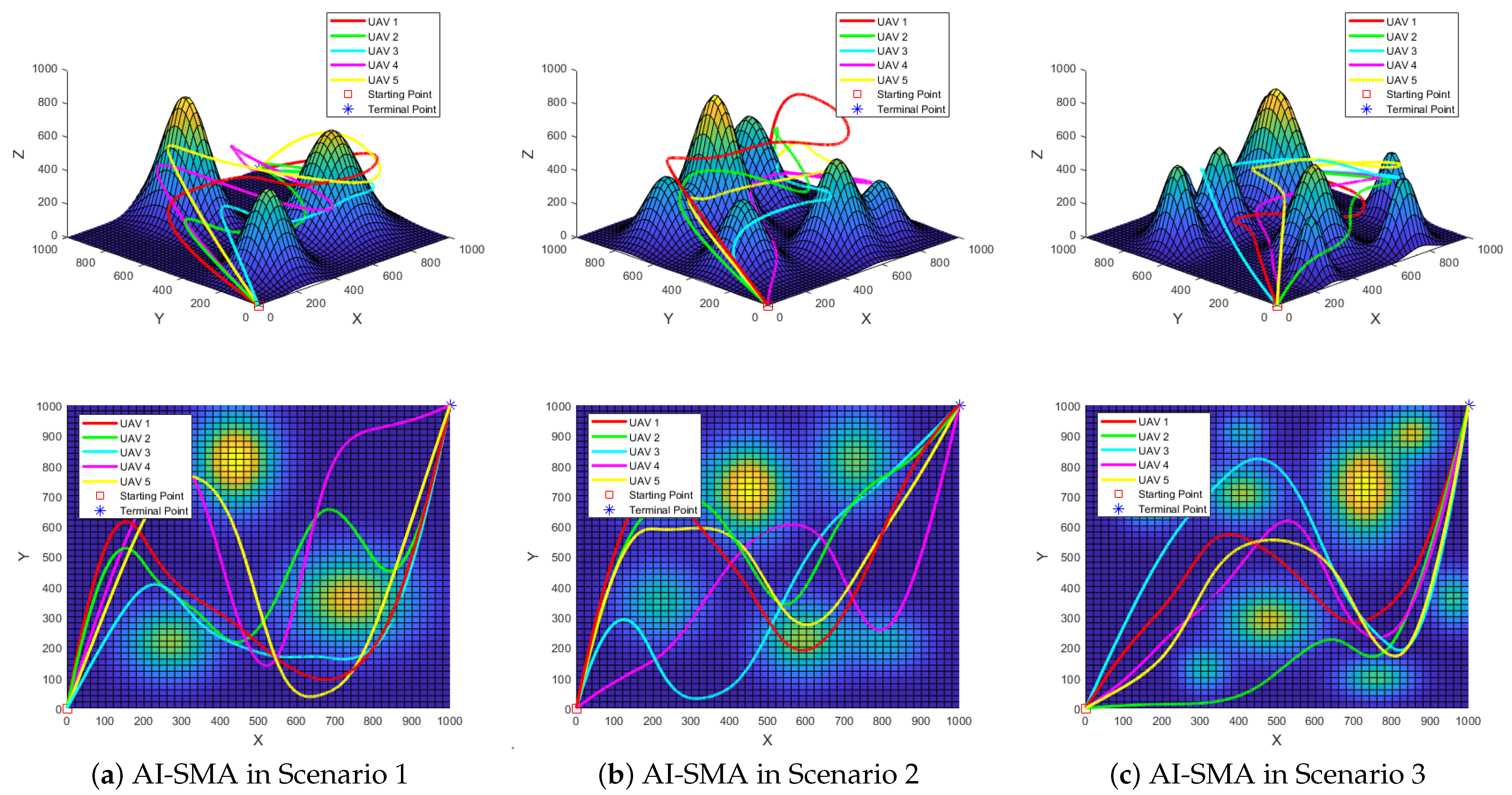
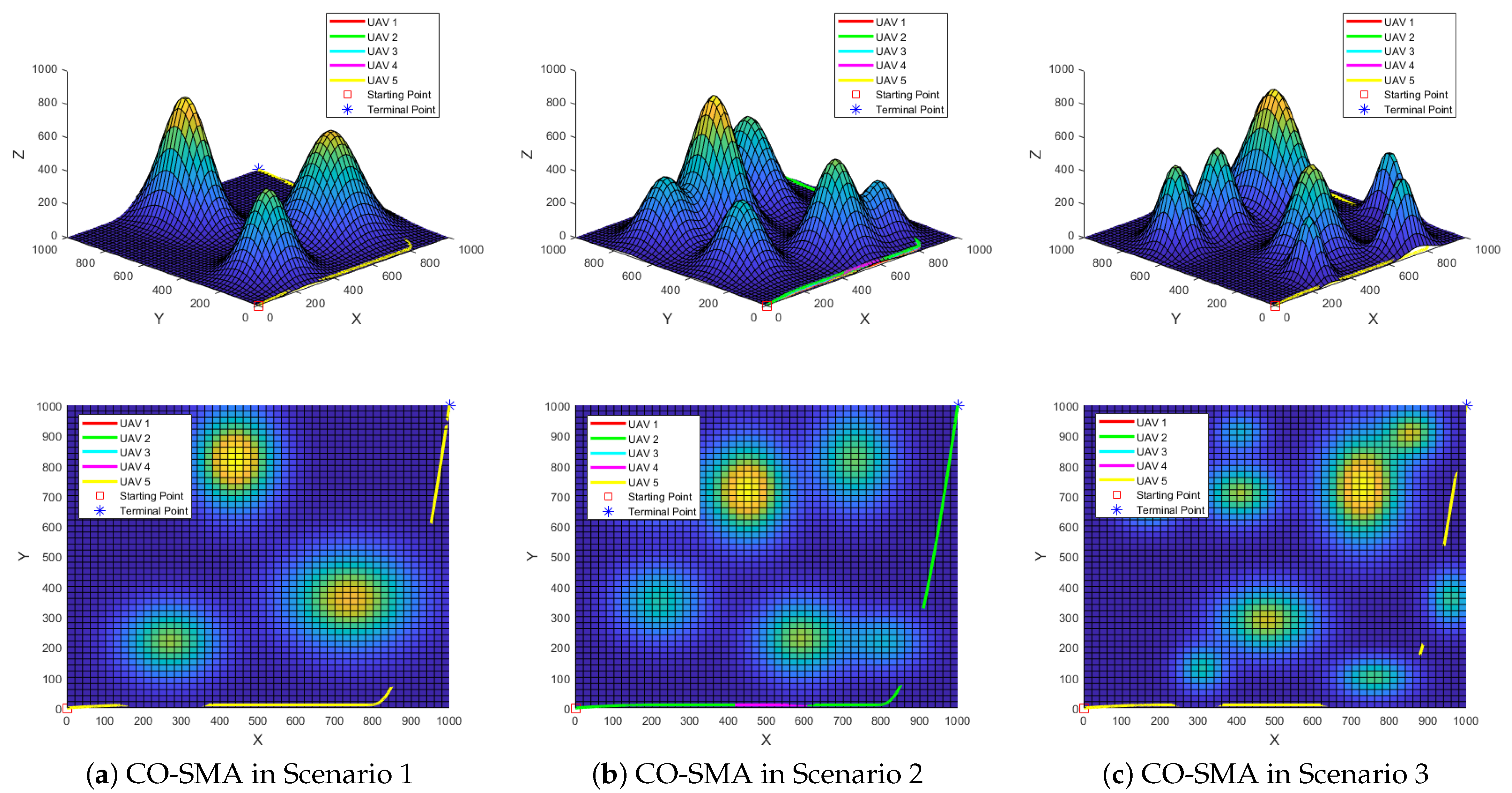
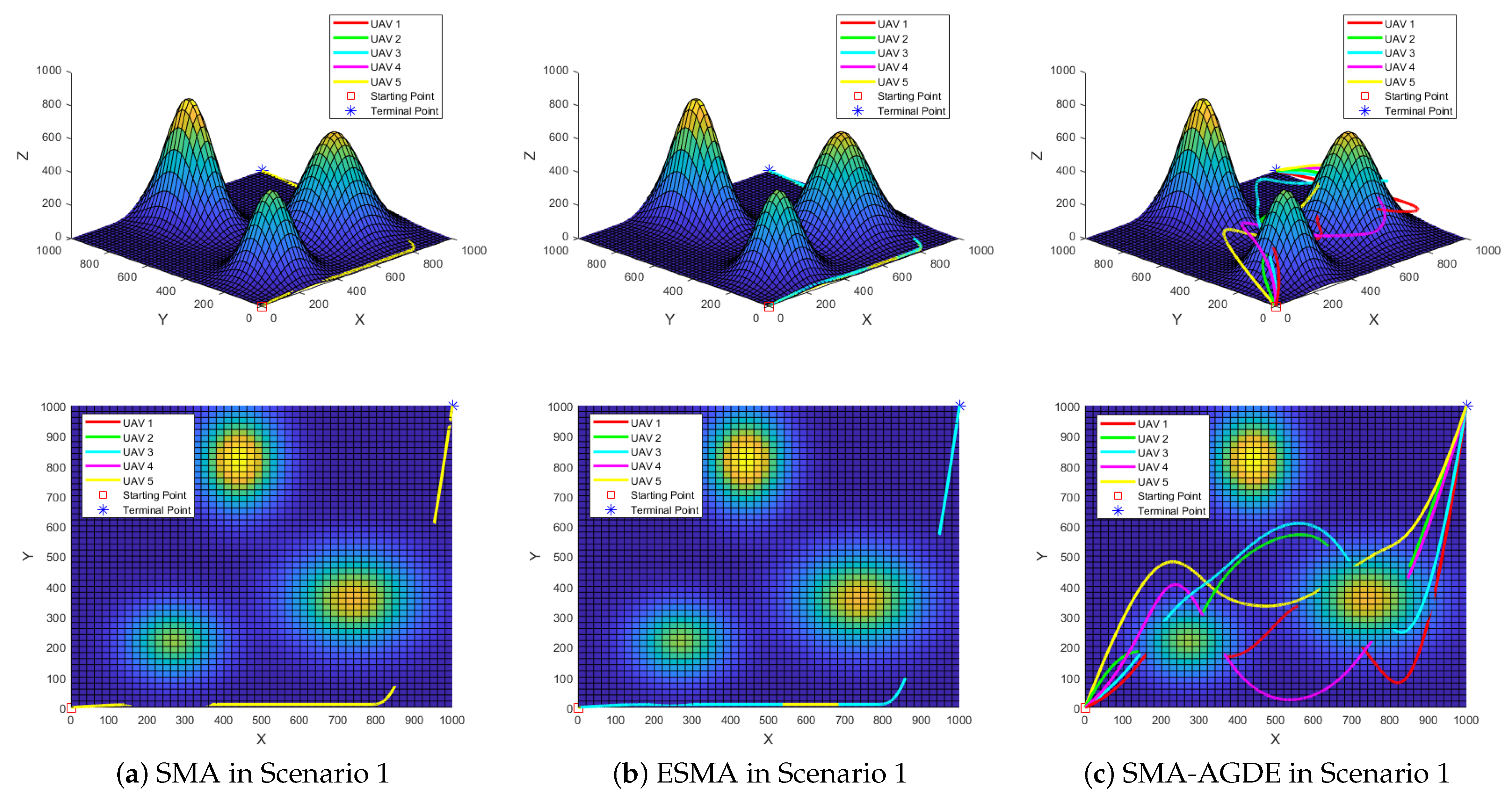
presents the comparative results of five algorithms across different scenarios. Figure 9 illustrates the average convergence curves for these algorithms. Figure 10 and Figure 11 display the best path-planning outcomes for the three-dimensional and two-dimensional views of AI-SMA and CO-SMA, respectively. The SMA, ESMA, and SMA-AGDE plots are provided in Appendix B. The red square indicates the starting point in these figures, while the blue star signifies the terminal point. Notably, in the two-dimensional plot, continuous curves indicate collision-free trajectories for UAVs, whereas any discontinuities highlight potential collision points. If a single curve is displayed, it indicates that the trajectories of all UAVs coincide.

In Scenario 1 with three obstacles, AI-SMA exhibits enhanced robustness, as evidenced by achieving optimal standard deviation and second-highest average fitness value among the evaluated algorithms in Table 7. Figure 9a confirms its competitive convergence performance, ranking second among the five algorithms. Trajectory results in Figure 11a and Figure A2a,b reveal that CO-SMA, SMA, and ESMA generate nearly identical flight trajectories for all UAVs, leading to UAV collisions at each waypoint due to insufficient safety distance. Additionally, two significant breaks in these curves indicate that all UAVs will experience severe collisions with obstacles. While SMA-AGDE avoids inter-UAV collisions, as shown in Figure A2c, it fails to prevent critical collisions with two obstacles. In contrast, AI-SMA generates collision-free trajectories for all UAVs except for a minor collision between UAV3 and one obstacle, as shown in Figure 10a. Therefore, AI-SMA is recognized as the best-performing algorithm in Scenario 1.

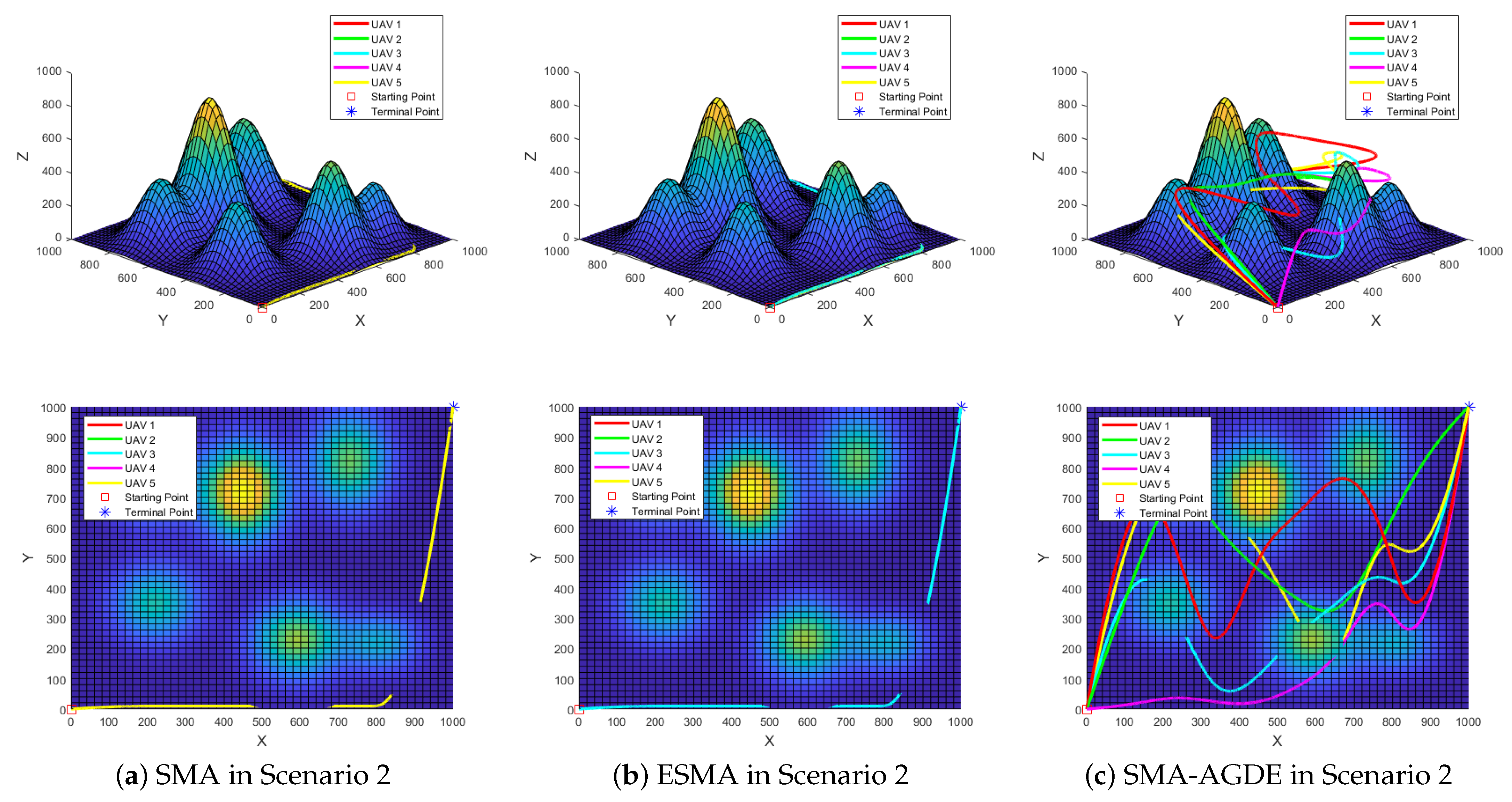
Compared to Scenario 1, Scenario 2 presents more obstacles and greater challenges. The results shown in Table 7 and Figure 9b indicate that AI-SMA performs best in this scenario. Specifically, AI-SMA achieves the best average fitness and standard deviation, along with superior convergence effectiveness. AI-SMA also successfully generates collision-free flight trajectories for all UAVs, as shown in Figure 10b. Conversely, UAV flight trajectories generated by the other four algorithms, as illustrated in Figure 11b and Figure A3a–c, are not feasible and will collide with obstacles. Consequently, the performance of AI-SMA in Scenario 2 is optimal as well.

Scenario 3 is the most complex, featuring the highest number and density of obstacles. As shown in Table 7 and Figure 9c, AI-SMA achieves the best standard deviation and second place in average fitness and convergence behavior, indicating that the algorithm remains robust even in the most complex scenarios. Furthermore, Figure 11c and Figure A4a–c demonstrate that the UAV flight trajectories generated by CO-SMA, SMA, ESMA, and SMA-AGDE are invalid, with an increase in collision points as scene complexity rises. Only AI-SMA, depicted in Figure 10c, produces complete, flyable, and collision-free flight trajectories, showcasing the excellent performance of the algorithm in Scenario 3.

Overall, the experimental results for multi-UAV path planning demonstrate that the proposed AI-SMA exhibits superior convergence properties, consistently ranking among the top two algorithms for both convergence speed and overall performance in all tested scenarios. Regarding robustness, AI-SMA achieves the best average fitness and standard deviation across varying densities of obstacles and terrains while generating flyable trajectories. Notably, AI-SMA is the only algorithm capable of producing collision-free trajectories for all UAVs in every scenario, while other algorithms often fail to generate feasible paths, leading to collisions with obstacles or other UAVs. Therefore, AI-SMA outperforms competing algorithms in terms of convergence effectiveness, robustness, and collision avoidance.

These advantages make AI-SMA particularly well-suited for real-world multi-UAV applications, such as search and rescue missions in mountainous terrains or firefight operations in densely populated urban environments, where reliable obstacle avoidance and robust performance are critical.

5.3. Strategy Validity Analysis

The proposed AI-SMA incorporates three strategies to improve the performance of SMA. To validate the effectiveness of each improvement, experiments were conducted on representative benchmark functions from CEC 2017 and Scenario 2 of multi-UAV path-planning problems. The following algorithms were considered for the experiment:

• SMA: the original SMA;
• SMA_S1: SMA with a novel search mechanism;
• SMA_S2: SMA with a self-adaptive switch operator;
• SMA_S3: SMA with a self-adaptive perturbation strategy;
• AI-SMA: SMA incorporating all three strategies.

All experimental settings and evaluation metrics remain consistent with Section 5.1.1 and Section 5.2. The experimental results for SMA, SMA_S1, SMA_S2, SMA_S3, and AI-SMA over 30 runs are summarized in

Table 8. Results of strategy validity experiments over 30 runs.

No.	Metrics	SMA	SMA_S1	SMA_S2	SMA_S3	AI-SMA
CEC 2017 benchmark test suite
$F_1$	BEST	$5.61\times {10}^4$	$2.77\times {10}^4$	$4.17\times {10}^{10}$	$5.41\times {10}^{10}$	$\mathbf{7.71}\times {\mathbf{10}}^{\mathbf{2}}$
	AVG	$\mathbf{4.85}\times {\mathbf{10}}^{\mathbf{4}}$	$1.03\times {10}^5$	$3.20\times {10}^{10}$	$4.26\times {10}^{10}$	$5.13\times {10}^4$
	STD	$\mathbf{5.46}\times {\mathbf{10}}^{\mathbf{4}}$	$1.76\times {10}^5$	$3.25\times {10}^{10}$	$4.40\times {10}^{10}$	$1.22\times {10}^5$
$F_3$	BEST *	$2.00\times {10}^2$	$2.00\times {10}^2$	$6.67\times {10}^4$	$1.02\times {10}^5$	$\mathbf{2.00}\times {\mathbf{10}}^{\mathbf{2}}$
	AVG	$\mathbf{1.08}\times {\mathbf{10}}^{\mathbf{2}}$	$1.57\times {10}^2$	$5.23\times {10}^4$	$7.06\times {10}^4$	$1.26\times {10}^2$
	STD	$\mathbf{9.34}\times {\mathbf{10}}^{\mathbf{1}}$	$1.86\times {10}^2$	$5.30\times {10}^4$	$7.21\times {10}^4$	$1.31\times {10}^2$
$F_5$	BEST	$5.19\times {10}^2$	$4.72\times {10}^2$	$6.60\times {10}^4$	$7.06\times {10}^4$	$\mathbf{4.59}\times {\mathbf{10}}^{\mathbf{2}}$
	AVG	$2.96\times {10}^2$	$2.70\times {10}^2$	$4.05\times {10}^4$	$5.23\times {10}^4$	$\mathbf{2.62}\times {\mathbf{10}}^{\mathbf{2}}$
	STD	$2.83\times {10}^2$	$2.58\times {10}^2$	$4.09\times {10}^4$	$5.33\times {10}^4$	$\mathbf{2.49}\times {\mathbf{10}}^{\mathbf{2}}$
$F_{10}$	BEST	$3.33\times {10}^3$	$3.07\times {10}^3$	$8.01\times {10}^3$	$8.48\times {10}^3$	$\mathbf{2.80}\times {\mathbf{10}}^{\mathbf{3}}$
	AVG	$2.20\times {10}^3$	$2.34\times {10}^3$	$4.30\times {10}^3$	$4.68\times {10}^3$	$\mathbf{2.05}\times {\mathbf{10}}^{\mathbf{3}}$
	STD	$2.23\times {10}^3$	$2.37\times {10}^3$	$4.29\times {10}^3$	$4.67\times {10}^3$	$\mathbf{2.09}\times {\mathbf{10}}^{\mathbf{3}}$
$F_{14}$	BEST	$7.00\times {10}^4$	$2.23\times {10}^5$	$1.68\times {10}^6$	$4.48\times {10}^6$	$\mathbf{3.33}\times {\mathbf{10}}^{\mathbf{4}}$
	AVG	$\mathbf{1.30}\times {\mathbf{10}}^{\mathbf{5}}$	$4.67\times {10}^5$	$3.13\times {10}^6$	$1.01\times {10}^7$	$1.59\times {10}^5$
	STD	$\mathbf{1.84}\times {\mathbf{10}}^{\mathbf{5}}$	$6.63\times {10}^5$	$3.64\times {10}^6$	$1.22\times {10}^7$	$2.27\times {10}^5$
$F_{20}$	BEST	$\mathbf{1.95}\times {\mathbf{10}}^{\mathbf{3}}$	$2.02\times {10}^3$	$8.45\times {10}^3$	$1.15\times {10}^4$	$2.01\times {10}^3$
	AVG	$\mathbf{1.15}\times {\mathbf{10}}^{\mathbf{3}}$	$1.36\times {10}^3$	$5.74\times {10}^3$	$9.16\times {10}^3$	$1.28\times {10}^3$
	STD	$\mathbf{1.15}\times {\mathbf{10}}^{\mathbf{3}}$	$1.38\times {10}^3$	$5.85\times {10}^3$	$9.43\times {10}^3$	$1.28\times {10}^3$
$F_{23}$	BEST	$2.44\times {10}^3$	$2.41\times {10}^3$	$4.34\times {10}^4$	$6.00\times {10}^4$	$\mathbf{2.39}\times {\mathbf{10}}^{\mathbf{3}}$
	AVG	$1.25\times {10}^3$	$\mathbf{1.22}\times {\mathbf{10}}^{\mathbf{3}}$	$3.01\times {10}^4$	$3.91\times {10}^4$	$1.23\times {10}^3$
	STD	$1.24\times {10}^3$	$\mathbf{1.20}\times {\mathbf{10}}^{\mathbf{3}}$	$3.05\times {10}^4$	$3.97\times {10}^4$	$1.22\times {10}^3$
$F_{29}$	BEST	$7.86\times {10}^3$	$3.88\times {10}^3$	$1.46\times {10}^9$	$6.15\times {10}^{10}$	$\mathbf{3.51}\times {\mathbf{10}}^{\mathbf{3}}$
	AVG	$4.28\times {10}^4$	$2.43\times {10}^3$	$2.44\times {10}^{11}$	$4.88\times {10}^{12}$	$\mathbf{2.20}\times {\mathbf{10}}^{\mathbf{3}}$
	STD	$8.25\times {10}^4$	$2.46\times {10}^3$	$7.42\times {10}^{11}$	$1.10\times {10}^{13}$	$\mathbf{2.20}\times {\mathbf{10}}^{\mathbf{3}}$
Multi-UAV path-planning problems
Scenario 2	BEST	$\mathbf{2.49}\times {\mathbf{10}}^{\mathbf{3}}$	$9.35\times {10}^3$	$3.71\times {10}^3$	$2.89\times {10}^3$	$3.84\times {10}^3$
	AVG	$8.70\times {10}^3$	$1.05\times {10}^4$	$7.22\times {10}^3$	$8.50\times {10}^3$	$\mathbf{4.84}\times {\mathbf{10}}^{\mathbf{3}}$
	STD	$2.03\times {10}^3$	$6.45\times {10}^2$	$1.90\times {10}^3$	$1.97\times {10}^3$	$\mathbf{4.80}\times {\mathbf{10}}^{\mathbf{2}}$

* The actual numerical values represented in scientific notation differ.

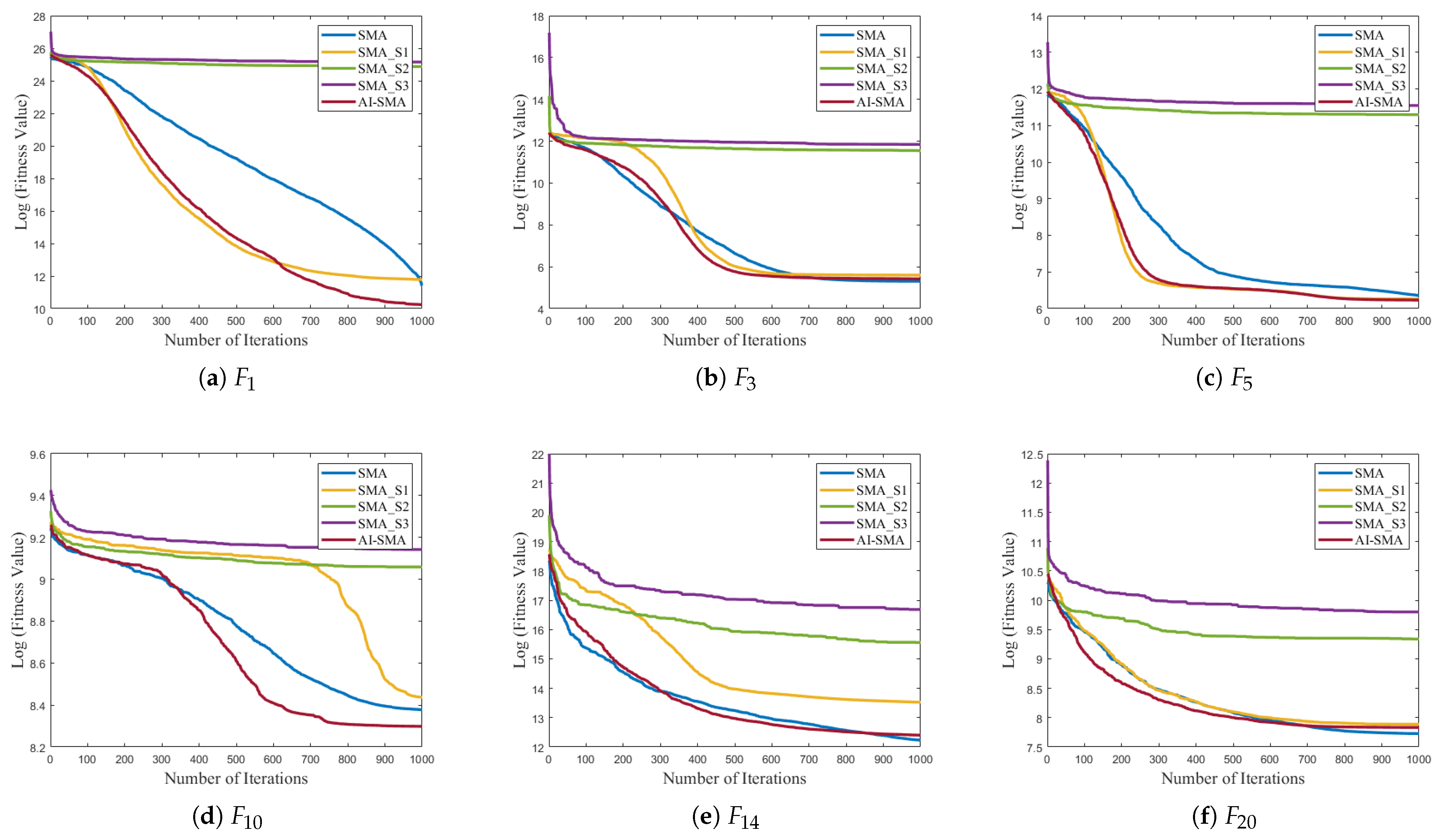
. The comparative effectiveness and the path-planning outcomes are illustrated in Figure 12 and Figure 13, respectively.

The results presented in Table 8 indicate that SMA_S1, which employs a novel search mechanism, achieves the best average fitness and standard deviation on $F_{23}$ in the CEC test suite. Moreover, its best fitness is superior to SMA on $F_1$, $F_5$, $F_{10}$, $F_{23}$, and $F_{29}$. SMA_S2 and SMA_S3, which utilize a self-adaptive switch operator and a self-adaptive perturbation strategy, demonstrate improved average fitness and standard deviation compared to the original SMA in Scenario 2. These findings demonstrate that the three enhancement strategies proposed in this paper contribute to varying degrees of numerical improvement in the performance of SMA.

Regarding convergence performance, Figure 12 illustrates that the convergence speed and effectiveness of SMA_S1 on $F_1$, $F_5$, $F_{23}$, $F_{29}$, and Scenario 2 are superior to SMA. Although the advantages of SMA_S2 and SMA_S3 are less pronounced in the CEC 2017 benchmark functions, both exhibit better convergence performance than SMA in Scenario 2 from the multi-UAV path-planning problems.

Figure 13a,b demonstrate that SMA_S1 and SMA_S2 can generate viable flight trajectories for the majority of UAVs. Despite some collisions within the paths, they represent a substantial advancement compared to the completely non-flyable trajectories produced by SMA, as shown in Figure A3a. Figure 13c illustrates that SMA_S3 offers limited assistance in generating a flyable path, primarily due to the inherent weak exploration capability of SMA, which restricts the effectiveness of the self-adaptive perturbation strategy. Nevertheless, the numerical and convergence analysis results collectively indicate that SMA_S3 enhances the effectiveness of SMA.

To sum up, the three strategies introduced in this paper have improved the exploration capabilities, convergence speed, and path-planning efficiency of the original SMA to some extent. After integrating the three strategies, the performance of AI-SMA proves to be superior to SMA in the CEC 2017 test suite and multi-UAV path-planning issues.

5.4. Parameter Experiments

AI-SMA has two key parameters: the Crossover Rate $Cr$ and the Perturbation Rate $\xi$. $Cr$ controls the position update patterns of individuals in the novel search mechanism, as expressed in Equation (33). $\xi$ denotes the population percentage that needs to be eliminated in the self-adaptive perturbation strategy, as shown in Equation (36).

In the proposed novel search mechanism, it is intended that most individuals locate the optimal value through positive–negative feedback related to food concentration, which aligns with the natural behavior of slime molds. Consequently, the minimum value of $Cr$ is set at 0.5. Additionally, to ensure that the integrated rank-DE mutation strategy contributes to the exploitation process, the maximum value of $Cr$ is set at 0.8.

Regarding the self-adaptive perturbation strategy, it is intended to avoid making large-scale adjustments to the population structure, so the value for $\xi$ is established between 0.1 and 0.2. This means the perturbation strategy will eliminate and update the worst-performing $10\%$ to $20\%$ of individuals.

Considering the requirements above, 8 parameter combinations were tested on the CEC 2017 benchmark test suite over 30 independent runs. The optimal combinations were selected based on rankings from the Friedman test. For parameter experiments, the population size ($NP$) and problem dimension ($Dim$) are set as 30, and the maximum iteration limitation ($t_{max}$) is configured to 1000. The Friedman test results are listed in

Table 9. The Friedman test results on CEC 2017 test suite with 30 Dim over 30 runs.

Friedman Test Results	(0.5, 0.1)	(0.5, 0.2)	(0.6, 0.1)	(0.6, 0.2)	(0.7, 0.1)	(0.7, 0.2)	(0.8, 0.1)	(0.8, 0.2)
Mean Rank	2.24	2.64	2.67	3.59	3.20	3.95	3.72	4.72
Rank	1	2	3	5	4	7	6	8

, with complete numerical results provided in

Table A1. Parameter experiments on CEC 2017 test suite with 30 Dim over 30 runs.

No.	Metrics	(0.5, 0.1)	(0.5, 0.2)	(0.6, 0.1)	(0.6, 0.2)	(0.7, 0.1)	(0.7, 0.2)	(0.8, 0.1)	(0.8, 0.2)
Unimodal Functions
$F_1$	BEST	$1.21\times {10}^3$	$\mathbf{4.67}\times {\mathbf{10}}^{\mathbf{2}}$	$3.64\times {10}^3$	$1.65\times {10}^4$	$3.04\times {10}^3$	$1.12\times {10}^4$	$1.53\times {10}^3$	$5.84\times {10}^2$
	AVG	$5.59\times {10}^4$	$2.26\times {10}^5$	$\mathbf{3.76}\times {\mathbf{10}}^{\mathbf{4}}$	$9.98\times {10}^4$	$5.24\times {10}^4$	$1.73\times {10}^5$	$7.60\times {10}^4$	$7.23\times {10}^4$
	STD	$1.21\times {10}^5$	$9.72\times {10}^5$	$\mathbf{8.40}\times {\mathbf{10}}^{\mathbf{4}}$	$1.89\times {10}^5$	$1.13\times {10}^5$	$3.67\times {10}^5$	$2.59\times {10}^5$	$1.45\times {10}^5$
$F_3$	BEST *	$2.00\times {10}^2$	$2.00\times {10}^2$	$2.00\times {10}^2$	$2.00\times {10}^2$	$\mathbf{2.00}\times {\mathbf{10}}^{\mathbf{2}}$	$2.00\times {10}^2$	$2.00\times {10}^2$	$2.00\times {10}^2$
	AVG	$\mathbf{1.14}\times {\mathbf{10}}^{\mathbf{2}}$	$1.40\times {10}^2$	$1.40\times {10}^2$	$1.30\times {10}^2$	$1.27\times {10}^2$	$1.15\times {10}^2$	$1.20\times {10}^2$	$1.15\times {10}^2$
	STD	$\mathbf{9.98}\times {\mathbf{10}}^{\mathbf{1}}$	$1.73\times {10}^2$	$2.05\times {10}^2$	$1.52\times {10}^2$	$1.30\times {10}^2$	$1.11\times {10}^2$	$1.23\times {10}^2$	$1.11\times {10}^2$
Simple Multi-modal Functions
$F_4$	BEST	$3.15\times {10}^2$	$3.20\times {10}^2$	$3.22\times {10}^2$	$\mathbf{3.10}\times {\mathbf{10}}^{\mathbf{2}}$	$3.17\times {10}^2$	$3.13\times {10}^2$	$3.17\times {10}^2$	$3.20\times {10}^2$
	AVG	$1.82\times {10}^2$	$1.86\times {10}^2$	$1.85\times {10}^2$	$1.84\times {10}^2$	$1.87\times {10}^2$	$\mathbf{1.78}\times {\mathbf{10}}^{\mathbf{2}}$	$1.81\times {10}^2$	$1.87\times {10}^2$
	STD	$1.70\times {10}^2$	$0.73\times {10}^2$	$1.72\times {10}^2$	$1.72\times {10}^2$	$1.75\times {10}^2$	$\mathbf{1.66}\times {\mathbf{10}}^{\mathbf{2}}$	$1.68\times {10}^2$	$1.74\times {10}^2$
$F_5$	BEST	$\mathbf{4.55}\times {\mathbf{10}}^{\mathbf{2}}$	$4.61\times {10}^2$	$4.73\times {10}^2$	$4.77\times {10}^2$	$4.87\times {10}^2$	$4.99\times {10}^2$	$4.96\times {10}^2$	$5.05\times {10}^2$
	AVG	$\mathbf{2.59}\times {\mathbf{10}}^{\mathbf{2}}$	$2.70\times {10}^2$	$2.64\times {10}^2$	$2.79\times {10}^2$	$2.77\times {10}^2$	$2.83\times {10}^2$	$2.76\times {10}^2$	$2.94\times {10}^2$
	STD	$\mathbf{2.45}\times {\mathbf{10}}^{\mathbf{2}}$	$2.56\times {10}^2$	$2.50\times {10}^2$	$2.66\times {10}^2$	$2.64\times {10}^2$	$2.70\times {10}^2$	$2.63\times {10}^2$	$2.80\times {10}^2$
$F_6$	BEST *	$5.00\times {10}^2$	$5.00\times {10}^2$	$\mathbf{5.00}\times {\mathbf{10}}^{\mathbf{2}}$	$5.00\times {10}^2$	$5.00\times {10}^2$	$5.00\times {10}^2$	$5.00\times {10}^2$	$5.00\times {10}^2$
	AVG *	$\mathbf{2.57}\times {\mathbf{10}}^{\mathbf{2}}$	$2.57\times {10}^2$	$2.57\times {10}^2$	$2.57\times {10}^2$	$2.57\times {10}^2$	$2.57\times {10}^2$	$2.57\times {10}^2$	$2.57\times {10}^2$
	STD *	$\mathbf{2.43}\times {\mathbf{10}}^{\mathbf{2}}$	$2.43\times {10}^2$	$2.43\times {10}^2$	$2.43\times {10}^2$	$2.43\times {10}^2$	$2.43\times {10}^2$	$2.43\times {10}^2$	$2.43\times {10}^2$
$F_7$	BEST	$7.22\times {10}^2$	$7.60\times {10}^2$	$7.22\times {10}^2$	$7.60\times {10}^2$	$\mathbf{6.91}\times {\mathbf{10}}^{\mathbf{2}}$	$7.95\times {10}^2$	$7.66\times {10}^2$	$8.12\times {10}^2$
	AVG	$\mathbf{3.95}\times {\mathbf{10}}^{\mathbf{2}}$	$4.23\times {10}^2$	$4.04\times {10}^2$	$4.51\times {10}^2$	$4.04\times {10}^2$	$4.61\times {10}^2$	$4.30\times {10}^2$	$4.71\times {10}^2$
	STD	$\mathbf{3.81}\times {\mathbf{10}}^{\mathbf{2}}$	$4.10\times {10}^2$	$3.90\times {10}^2$	$4.38\times {10}^2$	$3.92\times {10}^2$	$4.48\times {10}^2$	$4.17\times {10}^2$	$4.58\times {10}^2$
$F_8$	BEST	$\mathbf{7.72}\times {\mathbf{10}}^{\mathbf{2}}$	$8.18\times {10}^2$	$7.96\times {10}^2$	$8.26\times {10}^2$	$8.42\times {10}^2$	$8.12\times {10}^2$	$8.10\times {10}^2$	$8.60\times {10}^2$
	AVG	$\mathbf{4.46}\times {\mathbf{10}}^{\mathbf{2}}$	$4.60\times {10}^2$	$4.57\times {10}^2$	$4.61\times {10}^2$	$4.69\times {10}^2$	$4.61\times {10}^2$	$4.60\times {10}^2$	$4.84\times {10}^2$
	STD	$\mathbf{4.33}\times {\mathbf{10}}^{\mathbf{2}}$	$4.48\times {10}^2$	$4.43\times {10}^2$	$4.48\times {10}^2$	$4.56\times {10}^2$	$4.48\times {10}^2$	$4.48\times {10}^2$	$4.72\times {10}^2$
$F_9$	BEST *	$\mathbf{8.00}\times {\mathbf{10}}^{\mathbf{2}}$	$8.00\times {10}^2$	$8.00\times {10}^2$	$8.00\times {10}^2$	$8.01\times {10}^2$	$8.01\times {10}^2$	$8.01\times {10}^2$	$8.01\times {10}^2$
	AVG *	$4.09\times {10}^2$	$\mathbf{4.09}\times {\mathbf{10}}^{\mathbf{2}}$	$4.09\times {10}^2$	$4.09\times {10}^2$	$4.09\times {10}^2$	$4.09\times {10}^2$	$4.10\times {10}^2$	$4.09\times {10}^2$
	STD *	$3.95\times {10}^2$	$\mathbf{3.94}\times {\mathbf{10}}^{\mathbf{2}}$	$3.94\times {10}^2$	$3.95\times {10}^2$	$3.95\times {10}^2$	$3.95\times {10}^2$	$3.95\times {10}^2$	$3.95\times {10}^2$
$F_{10}$	BEST	$2.86\times {10}^3$	$\mathbf{2.40}\times {\mathbf{10}}^{\mathbf{3}}$	$2.86\times {10}^3$	$2.75\times {10}^3$	$2.88\times {10}^3$	$2.92\times {10}^3$	$2.78\times {10}^3$	$3.28\times {10}^3$
	AVG	$2.04\times {10}^3$	$2.03\times {10}^3$	$2.15\times {10}^3$	$\mathbf{1.95}\times {\mathbf{10}}^{\mathbf{3}}$	$2.15\times {10}^3$	$2.04\times {10}^3$	$2.14\times {10}^3$	$2.18\times {10}^3$
	STD	$2.08\times {10}^3$	$2.06\times {10}^3$	$2.20\times {10}^3$	$\mathbf{2.00}\times {\mathbf{10}}^{\mathbf{3}}$	$2.19\times {10}^3$	$2.09\times {10}^3$	$2.22\times {10}^3$	$2.20\times {10}^3$
Hybrid Functions
$F_{11}$	BEST	$1.51\times {10}^4$	$8.72\times {10}^3$	$2.14\times {10}^4$	$\mathbf{7.44}\times {\mathbf{10}}^{\mathbf{3}}$	$1.73\times {10}^4$	$1.93\times {10}^4$	$1.87\times {10}^4$	$1.94\times {10}^4$
	AVG	$4.22\times {10}^4$	$\mathbf{3.75}\times {\mathbf{10}}^{\mathbf{4}}$	$4.33\times {10}^4$	$6.05\times {10}^4$	$7.00\times {10}^4$	$4.28\times {10}^4$	$5.66\times {10}^4$	$4.32\times {10}^4$
	STD	$5.48\times {10}^4$	$\mathbf{5.00}\times {\mathbf{10}}^{\mathbf{4}}$	$5.82\times {10}^4$	$1.18\times {10}^5$	$1.48\times {10}^5$	$5.80\times {10}^4$	$1.63\times {10}^5$	$5.91\times {10}^4$
$F_{12}$	BEST	$2.72\times {10}^5$	$1.02\times {10}^5$	$2.01\times {10}^5$	$\mathbf{9.19}\times {\mathbf{10}}^{\mathbf{4}}$	$7.06\times {10}^5$	$4.02\times {10}^5$	$2.13\times {10}^5$	$6.17\times {10}^5$
	AVG	$2.81\times {10}^6$	$2.90\times {10}^6$	$2.26\times {10}^6$	$2.43\times {10}^6$	$2.30\times {10}^6$	$\mathbf{2.01}\times {\mathbf{10}}^{\mathbf{6}}$	$2.81\times {10}^6$	$2.40\times {10}^6$
	STD	$4.21\times {10}^6$	$5.58\times {10}^6$	$\mathbf{3.30}\times {\mathbf{10}}^{\mathbf{6}}$	$3.78\times {10}^6$	$3.43\times {10}^6$	$3.57\times {10}^6$	$4.61\times {10}^6$	$3.66\times {10}^6$
$F_{13}$	BEST	$\mathbf{5.77}\times {\mathbf{10}}^{\mathbf{3}}$	$8.85\times {10}^3$	$2.23\times {10}^4$	$1.78\times {10}^4$	$1.05\times {10}^4$	$1.98\times {10}^4$	$1.60\times {10}^4$	$2.09\times {10}^4$
	AVG	$1.42\times {10}^5$	$\mathbf{6.84}\times {\mathbf{10}}^{\mathbf{4}}$	$1.18\times {10}^5$	$2.65\times {10}^5$	$1.19\times {10}^5$	$1.55\times {10}^5$	$1.81\times {10}^5$	$3.57\times {10}^5$
	STD	$3.29\times {10}^5$	$\mathbf{1.24}\times {\mathbf{10}}^{\mathbf{5}}$	$2.39\times {10}^5$	$7.41\times {10}^5$	$2.72\times {10}^5$	$2.96\times {10}^5$	$4.16\times {10}^5$	$9.22\times {10}^5$
$F_{14}$	BEST	$4.21\times {10}^4$	$5.06\times {10}^4$	$\mathbf{3.07}\times {\mathbf{10}}^{\mathbf{4}}$	$3.48\times {10}^4$	$3.99\times {10}^4$	$4.26\times {10}^4$	$5.35\times {10}^4$	$3.80\times {10}^4$
	AVG	$1.48\times {10}^5$	$1.85\times {10}^5$	$\mathbf{1.30}\times {\mathbf{10}}^{\mathbf{5}}$	$1.45\times {10}^5$	$1.41\times {10}^5$	$1.55\times {10}^5$	$1.39\times {10}^5$	$1.53\times {10}^5$
	STD	$2.50\times {10}^5$	$2.78\times {10}^5$	$2.00\times {10}^5$	$2.27\times {10}^5$	$1.95\times {10}^5$	$2.44\times {10}^5$	$\mathbf{1.91}\times {\mathbf{10}}^{\mathbf{5}}$	$2.48\times {10}^5$
$F_{15}$	BEST	$2.11\times {10}^4$	$\mathbf{1.11}\times {\mathbf{10}}^{\mathbf{4}}$	$1.97\times {10}^4$	$2.97\times {10}^4$	$1.50\times {10}^4$	$1.32\times {10}^4$	$1.63\times {10}^4$	$1.56\times {10}^4$
	AVG	$\mathbf{4.11}\times {\mathbf{10}}^{\mathbf{4}}$	$5.54\times {10}^4$	$4.93\times {10}^4$	$7.39\times {10}^4$	$7.29\times {10}^4$	$7.26\times {10}^4$	$6.18\times {10}^4$	$8.87\times {10}^4$
	STD	$\mathbf{5.32}\times {\mathbf{10}}^{\mathbf{4}}$	$1.17\times {10}^5$	$9.45\times {10}^4$	$1.40\times {10}^5$	$2.03\times {10}^5$	$1.66\times {10}^5$	$1.19\times {10}^5$	$2.37\times {10}^5$
$F_{16}$	BEST *	$2.80\times {10}^3$	$3.21\times {10}^3$	$\mathbf{2.66}\times {\mathbf{10}}^{\mathbf{3}}$	$3.05\times {10}^3$	$2.66\times {10}^3$	$3.56\times {10}^3$	$3.01\times {10}^3$	$2.96\times {10}^3$
	AVG	$\mathbf{3.39}\times {\mathbf{10}}^{\mathbf{3}}$	$3.86\times {10}^3$	$4.43\times {10}^3$	$4.58\times {10}^3$	$4.83\times {10}^3$	$3.46\times {10}^3$	$6.18\times {10}^3$	$4.48\times {10}^3$
	STD	$4.40\times {10}^3$	$6.52\times {10}^3$	$7.69\times {10}^3$	$8.72\times {10}^3$	$9.22\times {10}^3$	$\mathbf{4.34}\times {\mathbf{10}}^{\mathbf{3}}$	$1.37\times {10}^4$	$7.34\times {10}^3$
$F_{17}$	BEST	$\mathbf{1.89}\times {\mathbf{10}}^{\mathbf{3}}$	$1.95\times {10}^3$	$2.14\times {10}^3$	$2.30\times {10}^3$	$2.07\times {10}^3$	$2.24\times {10}^3$	$2.29\times {10}^3$	$1.90\times {10}^3$
	AVG	$\mathbf{1.48}\times {\mathbf{10}}^{\mathbf{3}}$	$1.51\times {10}^3$	$1.59\times {10}^3$	$1.66\times {10}^3$	$1.68\times {10}^3$	$1.69\times {10}^3$	$1.59\times {10}^3$	$1.64\times {10}^3$
	STD	$\mathbf{1.52}\times {\mathbf{10}}^{\mathbf{3}}$	$1.55\times {10}^3$	$1.62\times {10}^3$	$1.69\times {10}^3$	$1.70\times {10}^3$	$1.71\times {10}^3$	$1.61\times {10}^3$	$1.69\times {10}^3$
$F_{18}$	BEST	$5.55\times {10}^4$	$4.42\times {10}^4$	$6.22\times {10}^4$	$3.60\times {10}^4$	$5.27\times {10}^4$	$5.30\times {10}^4$	$\mathbf{3.22}\times {\mathbf{10}}^{\mathbf{4}}$	$7.28\times {10}^4$
	AVG	$\mathbf{8.94}\times {\mathbf{10}}^{\mathbf{4}}$	$9.97\times {10}^4$	$1.15\times {10}^5$	$1.19\times {10}^5$	$1.14\times {10}^5$	$1.47\times {10}^5$	$1.01\times {10}^5$	$1.39\times {10}^5$
	STD	$\mathbf{1.19}\times {\mathbf{10}}^{\mathbf{5}}$	$1.40\times {10}^5$	$1.94\times {10}^5$	$1.98\times {10}^5$	$2.00\times {10}^5$	$3.47\times {10}^5$	$1.35\times {10}^5$	$1.90\times {10}^5$
$F_{19}$	BEST	$6.66\times {10}^4$	$4.98\times {10}^3$	$2.01\times {10}^3$	$\mathbf{1.90}\times {\mathbf{10}}^{\mathbf{3}}$	$1.94\times {10}^3$	$1.93\times {10}^3$	$2.81\times {10}^3$	$2.09\times {10}^3$
	AVG	$9.59\times {10}^5$	$1.85\times {10}^6$	$\mathbf{9.33}\times {\mathbf{10}}^{\mathbf{5}}$	$2.22\times {10}^6$	$3.61\times {10}^6$	$6.18\times {10}^6$	$4.21\times {10}^6$	$6.00\times {10}^6$
	STD	$\mathbf{2.25}\times {\mathbf{10}}^{\mathbf{6}}$	$6.81\times {10}^6$	$2.36\times {10}^6$	$6.97\times {10}^6$	$8.36\times {10}^6$	$2.79\times {10}^7$	$1.29\times {10}^7$	$2.88\times {10}^7$
$F_{20}$	BEST	$1.98\times {10}^3$	$\mathbf{1.94}\times {\mathbf{10}}^{\mathbf{3}}$	$1.95\times {10}^3$	$2.20\times {10}^3$	$2.08\times {10}^3$	$2.19\times {10}^3$	$1.98\times {10}^3$	$2.11\times {10}^3$
	AVG	$\mathbf{1.24}\times {\mathbf{10}}^{\mathbf{3}}$	$1.25\times {10}^3$	$1.29\times {10}^3$	$1.31\times {10}^3$	$1.32\times {10}^3$	$1.35\times {10}^3$	$1.41\times {10}^3$	$1.37\times {10}^3$
	STD	$\mathbf{1.24}\times {\mathbf{10}}^{\mathbf{3}}$	$1.26\times {10}^3$	$1.29\times {10}^3$	$1.31\times {10}^3$	$1.33\times {10}^3$	$1.35\times {10}^3$	$1.47\times {10}^3$	$1.38\times {10}^3$
Composition Functions
$F_{21}$	BEST *	$2.11\times {10}^3$	$2.10\times {10}^3$	$\mathbf{2.10}\times {\mathbf{10}}^{\mathbf{3}}$	$2.11\times {10}^3$	$2.10\times {10}^3$	$2.11\times {10}^3$	$2.10\times {10}^3$	$2.11\times {10}^3$
	AVG	$1.12\times {10}^3$	$1.11\times {10}^3$	$1.11\times {10}^3$	$1.13\times {10}^3$	$\mathbf{1.08}\times {\mathbf{10}}^{\mathbf{3}}$	$1.11\times {10}^3$	$1.14\times {10}^3$	$1.10\times {10}^3$
	STD	$1.10\times {10}^3$	$1.09\times {10}^3$	$1.09\times {10}^3$	$1.11\times {10}^3$	$\mathbf{1.07}\times {\mathbf{10}}^{\mathbf{3}}$	$1.09\times {10}^3$	$1.13\times {10}^3$	$1.09\times {10}^3$
$F_{22}$	BEST *	$2.26\times {10}^3$	$\mathbf{2.26}\times {\mathbf{10}}^{\mathbf{3}}$	$2.26\times {10}^3$	$2.26\times {10}^3$	$2.26\times {10}^3$	$2.27\times {10}^3$	$2.26\times {10}^3$	$2.27\times {10}^3$
	AVG *	$1.14\times {10}^3$	$1.14\times {10}^3$	$\mathbf{1.14}\times {\mathbf{10}}^{\mathbf{3}}$	$1.14\times {10}^3$	$1.14\times {10}^3$	$1.14\times {10}^3$	$1.14\times {10}^3$	$1.15\times {10}^3$
	STD *	$1.13\times {10}^3$	$1.13\times {10}^3$	$\mathbf{1.13}\times {\mathbf{10}}^{\mathbf{3}}$	$1.13\times {10}^3$	$1.13\times {10}^3$	$1.13\times {10}^3$	$1.13\times {10}^3$	$1.13\times {10}^3$
$F_{23}$	BEST	$2.40\times {10}^3$	$2.42\times {10}^3$	$2.40\times {10}^3$	$2.41\times {10}^3$	$2.41\times {10}^3$	$2.42\times {10}^3$	$2.41\times {10}^3$	$\mathbf{2.36}\times {\mathbf{10}}^{\mathbf{3}}$
	AVG *	$1.23\times {10}^3$	$1.25\times {10}^3$	$1.24\times {10}^3$	$1.23\times {10}^3$	$1.24\times {10}^3$	$1.25\times {10}^3$	$\mathbf{1.23}\times {\mathbf{10}}^{\mathbf{3}}$	$1.26\times {10}^3$
	STD	$1.22\times {10}^3$	$1.23\times {10}^3$	$1.22\times {10}^3$	$1.22\times {10}^3$	$1.22\times {10}^3$	$1.24\times {10}^3$	$\mathbf{1.21}\times {\mathbf{10}}^{\mathbf{3}}$	$1.25\times {10}^3$
$F_{24}$	BEST	$2.50\times {10}^3$	$2.51\times {10}^3$	$2.50\times {10}^3$	$2.50\times {10}^3$	$2.50\times {10}^3$	$\mathbf{2.42}\times {\mathbf{10}}^{\mathbf{3}}$	$2.50\times {10}^3$	$2.50\times {10}^3$
	AVG *	$\mathbf{1.27}\times {\mathbf{10}}^{\mathbf{3}}$	$1.28\times {10}^3$	$1.27\times {10}^3$	$1.28\times {10}^3$	$1.27\times {10}^3$	$1.27\times {10}^3$	$1.27\times {10}^3$	$1.28\times {10}^3$
	STD *	$\mathbf{1.25}\times {\mathbf{10}}^{\mathbf{3}}$	$1.27\times {10}^3$	$1.26\times {10}^3$	$1.26\times {10}^3$	$1.26\times {10}^3$	$1.26\times {10}^3$	$1.25\times {10}^3$	$1.26\times {10}^3$
$F_{25}$	BEST *	$2.76\times {10}^3$	$\mathbf{2.76}\times {\mathbf{10}}^{\mathbf{3}}$	$2.76\times {10}^3$	$2.76\times {10}^3$	$2.76\times {10}^3$	$2.76\times {10}^3$	$2.76\times {10}^3$	$2.76\times {10}^3$
	AVG *	$1.39\times {10}^3$	$1.39\times {10}^3$	$1.39\times {10}^3$	$1.39\times {10}^3$	$\mathbf{1.39}\times {\mathbf{10}}^{\mathbf{3}}$	$1.39\times {10}^3$	$1.39\times {10}^3$	$1.39\times {10}^3$
	STD *	$1.38\times {10}^3$	$1.38\times {10}^3$	$1.38\times {10}^3$	$1.38\times {10}^3$	$\mathbf{1.38}\times {\mathbf{10}}^{\mathbf{3}}$	$1.38\times {10}^3$	$1.38\times {10}^3$	$1.38\times {10}^3$
$F_{26}$	BEST *	$\mathbf{2.91}\times {\mathbf{10}}^{\mathbf{3}}$	$2.91\times {10}^3$	$2.91\times {10}^3$	$2.91\times {10}^3$	$2.91\times {10}^3$	$2.91\times {10}^3$	$2.91\times {10}^3$	$2.91\times {10}^3$
	AVG	$1.47\times {10}^3$	$\mathbf{1.46}\times {\mathbf{10}}^{\mathbf{3}}$	$1.47\times {10}^3$	$1.47\times {10}^3$	$1.47\times {10}^3$	$1.47\times {10}^3$	$1.47\times {10}^3$	$1.47\times {10}^3$
	STD *	$1.45\times {10}^3$	$\mathbf{1.45}\times {\mathbf{10}}^{\mathbf{3}}$	$1.45\times {10}^3$	$1.45\times {10}^3$	$1.45\times {10}^3$	$1.45\times {10}^3$	$1.45\times {10}^3$	$1.45\times {10}^3$
$F_{27}$	BEST *	$3.10\times {10}^3$	$3.10\times {10}^3$	$3.10\times {10}^3$	$3.10\times {10}^3$	$3.10\times {10}^3$	$\mathbf{3.10}\times {\mathbf{10}}^{\mathbf{3}}$	$3.10\times {10}^3$	$3.10\times {10}^3$
	AVG *	$1.56\times {10}^3$	$1.56\times {10}^3$	$1.56\times {10}^3$	$1.56\times {10}^3$	$1.56\times {10}^3$	$\mathbf{1.56}\times {\mathbf{10}}^{\mathbf{3}}$	$1.56\times {10}^3$	$1.56\times {10}^3$
	STD *	$1.54\times {10}^3$	$1.54\times {10}^3$	$1.54\times {10}^3$	$1.54\times {10}^3$	$1.54\times {10}^3$	$\mathbf{1.54}\times {\mathbf{10}}^{\mathbf{3}}$	$1.54\times {10}^3$	$1.54\times {10}^3$
$F_{28}$	BEST	$3.20\times {10}^3$	$3.20\times {10}^3$	$3.20\times {10}^3$	$3.20\times {10}^3$	$\mathbf{3.19}\times {\mathbf{10}}^{\mathbf{3}}$	$3.20\times {10}^3$	$3.20\times {10}^3$	$3.20\times {10}^3$
	AVG *	$1.61\times {10}^3$	$\mathbf{1.61}\times {\mathbf{10}}^{\mathbf{3}}$	$1.61\times {10}^3$	$1.61\times {10}^3$	$1.61\times {10}^3$	$1.61\times {10}^3$	$1.61\times {10}^3$	$1.61\times {10}^3$
	STD *	$1.59\times {10}^3$	$\mathbf{1.59}\times {\mathbf{10}}^{\mathbf{3}}$	$1.59\times {10}^3$	$1.59\times {10}^3$	$1.59\times {10}^3$	$1.59\times {10}^3$	$1.59\times {10}^3$	$1.59\times {10}^3$
$F_{29}$	BEST	$\mathbf{3.40}\times {\mathbf{10}}^{\mathbf{3}}$	$3.51\times {10}^3$	$3.58\times {10}^3$	$3.51\times {10}^3$	$3.50\times {10}^3$	$3.73\times {10}^3$	$3.69\times {10}^3$	$3.45\times {10}^3$
	AVG	$2.31\times {10}^3$	$\mathbf{2.14}\times {\mathbf{10}}^{\mathbf{3}}$	$2.22\times {10}^3$	$2.30\times {10}^3$	$2.21\times {10}^3$	$2.26\times {10}^3$	$2.31\times {10}^3$	$2.29\times {10}^3$
	STD	$2.33\times {10}^3$	$\mathbf{2.15}\times {\mathbf{10}}^{\mathbf{3}}$	$2.23\times {10}^3$	$2.32\times {10}^3$	$2.23\times {10}^3$	$2.28\times {10}^3$	$2.33\times {10}^3$	$2.30\times {10}^3$
$F_{30}$	BEST	$3.51\times {10}^3$	$3.49\times {10}^3$	$\mathbf{3.19}\times {\mathbf{10}}^{\mathbf{3}}$	$3.25\times {10}^3$	$3.31\times {10}^3$	$3.48\times {10}^3$	$4.31\times {10}^3$	$3.39\times {10}^3$
	AVG	$1.71\times {10}^5$	$5.48\times {10}^4$	$5.76\times {10}^4$	$8.11\times {10}^4$	$\mathbf{5.08}\times {\mathbf{10}}^{\mathbf{4}}$	$6.11\times {10}^4$	$1.09\times {10}^5$	$1.00\times {10}^5$
	STD	$4.46\times {10}^5$	$2.01\times {10}^5$	$\mathbf{1.19}\times {\mathbf{10}}^{\mathbf{5}}$	$2.32\times {10}^5$	$1.38\times {10}^5$	$1.93\times {10}^5$	$2.71\times {10}^5$	$3.11\times {10}^5$

* The actual numerical values represented in scientific notation differ.

in Appendix C. The table column names are denoted as $(Cr,\xi )$.

Table 9 shows that the parameter combination of $Cr=0.5$ and $\xi =0.1$ ranked first among all combinations, making it the optimal choice for subsequent experiments.

6. Conclusions

This study proposes a self-adaptive improved slime mold algorithm (AI-SMA) to address the limitations of the original SMA and apply it to multi-UAV path-planning problems. Initially, to balance exploration and exploitation phases, a novel search mechanism is introduced that utilizes the robust exploration capabilities of rank-DE while enhancing the exploitation strengths of SMA. Next, a self-adaptive switch operator S replaced the fixed parameter z to ensure population diversity in later iterations and help prevent premature convergence. Lastly, a self-adaptive perturbation strategy is implemented to assist the algorithm in escaping local optima and to accelerate its convergence speed. The cubic B-spline curves are applied to smooth the flight trajectories produced by AI-SMA, further improving their feasibility.

The performance of AI-SMA is evaluated on the CEC 2017 benchmark test suite and three multi-UAV path-planning scenarios. Simulation results demonstrate that AI-SMA surpasses seven competitive meta-heuristic algorithms on the benchmark functions, achieving superior performance in optimal fitness value and convergence speed. In particular, AI-SMA improves approximately $7.83\%$ in the quality of optimal fitness over the original SMA. Compared to SMA and its three variants, AI-SMA exhibits enhanced convergence speed and robustness, and it is the only algorithm capable of generating collision-free trajectories. Furthermore, an analysis of computational complexity indicates that AI-SMA has a complexity similar to SMA. Strategy validity experiments also confirm that each of the three enhancements significantly improves the performance of SMA.

Beyond these immediate performance benefits, the findings of this study have broader implications for multi-UAV path-planning challenges. The capability of AI-SMA to generate collision-free trajectories creates new opportunities for UAV operations in complex and unstructured settings, such as disaster response and geological exploration. However, AI-SMA still has limitations compared to other meta-heuristic algorithms. For instance, the exploration method in the novel search mechanism relies on random distribution without enhancements, which may lead to longer search times for global optima. The self-adaptive perturbation strategy shows limited effectiveness in escaping local optima for multi-modal functions. Further improvements can focus on these areas to accelerate convergence speed and enhance effectiveness.

In addition, integrating AI-SMA with real-world unmanned aircraft systems presents a promising direction for future research. Transitioning from simulation to practical applications will pose challenges such as UAV battery power consumption, hardware adaptation, sensor accuracy, and communication limitations. Overcoming these challenges will enable more effective solutions to complex multi-UAV path-planning problems in real-world scenarios. This advancement will significantly enhance the applicability of AI-SMA in critical applications such as precision agriculture, traffic management, and industrial inspection.

References

1. Javed, S.; Hassan, A.; Ahmad, R.; Ahmed, W.; Ahmed, R.; Saadat, A.; Guizani, M. State-of-the-Art and Future Research Challenges in UAV Swarms. IEEE Internet Things J. 2024, 11, 19023–19045. [Google Scholar] [CrossRef]
2. Nawaz, H.; Ali, H.M.; Massan, S.-R. Applications of Unmanned Aerial Vehicles: A Review. 3C Tecnol. Innov. Apl. Pyme 2019, 85–105. [Google Scholar] [CrossRef]
3. Ma, L.; Lin, B.; Zhang, W.; Tao, J.; Zhu, X.; Chen, H. A Survey of Research on the Distributed Cooperation Method of the UAV Swarm Based on Swarm Intelligence. In Proceedings of the 2022 IEEE 13th International Conference on Software Engineering and Service Science (ICSESS), Beijing, China, 21–23 October 2022; pp. 305–309. [Google Scholar] [CrossRef]
4. Cao, P.; Lei, L.; Cai, S.; Shen, G.; Liu, X.; Wang, X.; Zhang, L.; Zhou, L.; Guizani, M. Computational Intelligence Algorithms for UAV Swarm Networking and Collaboration: A Comprehensive Survey and Future Directions. IEEE Commun. Surv. Tutor. 2024, 26, 2684–2728. [Google Scholar] [CrossRef]
5. Cui, J.; Wang, L.; Hu, B.; Chen, S. Incidence Control Units Selection Scheme to Enhance the Stability of Multiple UAVs Network. IEEE Internet Things J. 2022, 9, 13067–13076. [Google Scholar] [CrossRef]
6. Lyu, M.; Zhao, Y.; Huang, C.; Huang, H. Unmanned Aerial Vehicles for Search and Rescue: A Survey. Remote Sens. 2023, 15, 3266. [Google Scholar] [CrossRef]
7. Kumar, G.; Anwar, A.; Dikshit, A.; Poddar, A.; Soni, U.; Song, W.K. Obstacle Avoidance for a Swarm of Unmanned Aerial Vehicles Operating on Particle Swarm Optimization: A Swarm Intelligence Approach for Search and Rescue Missions. J. Braz. Soc. Mech. Sci. Eng. 2022, 44, 56. [Google Scholar] [CrossRef]
8. Qu, C.; Boubin, J.; Gafurov, D.; Zhou, J.; Aloysius, N.; Nguyen, H.; Calyam, P. UAV Swarms in Smart Agriculture: Experiences and Opportunities. In Proceedings of the 2022 IEEE 18th International Conference on e-Science (e-Science), Salt Lake City, UT, USA, 11–14 October 2022; pp. 148–158. [Google Scholar] [CrossRef]
9. Catala-Roman, P.; Segura-Garcia, J.; Dura, E.; Navarro-Camba, E.A.; Alcaraz-Calero, J.M.; Garcia-Pineda, M. AI-Based Autonomous UAV Swarm System for Weed Detection and Treatment: Enhancing Organic Orange Orchard Efficiency with Agriculture 5.0. Internet Things 2024, 28, 101418. [Google Scholar] [CrossRef]
10. Yang, Z.; Yu, X.; Dedman, S.; Rosso, M.; Zhu, J.; Yang, J.; Xia, Y.; Tian, Y.; Zhang, G.; Wang, J. UAV Remote Sensing Applications in Marine Monitoring: Knowledge Visualization and Review. Sci. Total Environ. 2022, 838, 155939. [Google Scholar] [CrossRef]
11. Asadzadeh, S.; de Oliveira, W.J.; de Souza Filho, C.R. UAV-Based Remote Sensing for the Petroleum Industry and Environmental Monitoring: State-of-the-Art and Perspectives. J. Pet. Sci. Eng. 2022, 208, 109633. [Google Scholar] [CrossRef]
12. Lyu, X.; Li, X.; Dang, D.; Dou, H.; Wang, K.; Lou, A. Unmanned Aerial Vehicle (UAV) Remote Sensing in Grassland Ecosystem Monitoring: A Systematic Review. Remote Sens. 2022, 14, 1096. [Google Scholar] [CrossRef]
13. Zhang, X.; Zheng, J.; Su, T.; Ding, M.; Liu, H. An Effective Dynamic Constrained Two-Archive Evolutionary Algorithm for Cooperative Search-Track Mission Planning by UAV Swarms in Air Intelligent Transportation. IEEE Trans. Intell. Transp. Syst. 2024, 25, 944–958. [Google Scholar] [CrossRef]
14. Bakirci, M. Enhancing Vehicle Detection in Intelligent Transportation Systems via Autonomous UAV Platform and YOLOv8 Integration. Appl. Soft Comput. 2024, 164, 112015. [Google Scholar] [CrossRef]
15. Li, X.; Gong, L.; Liu, X.; Jiang, F.; Shi, W.; Fan, L.; Gao, H.; Li, R.; Xu, J. Solving the Last Mile Problem in Logistics: A Mobile Edge Computing and Blockchain-Based Unmanned Aerial Vehicle Delivery System. Concurr. Comput. Pract. Exp. 2022, 34, e6068. [Google Scholar] [CrossRef]
16. Betti Sorbelli, F. UAV-Based Delivery Systems: A Systematic Review, Current Trends, and Research Challenges. ACM J. Auton. Transp. Syst. 2024, 1, 12:1–12:40. [Google Scholar] [CrossRef]
17. Jyoti, J.; Batth, R.S. Unmanned Aerial Vehicles (UAV) Path Planning Approaches. In Proceedings of the 2021 International Conference on Computing Sciences (ICCS), Phagwara, India, 4–5 December 2021; pp. 76–82. [Google Scholar] [CrossRef]
18. Besada-Portas, E.; De La Torre, L.; De La Cruz, J.M.; De Andrés-Toro, B. Evolutionary Trajectory Planner for Multiple UAVs in Realistic Scenarios. IEEE Trans. Robot. 2010, 26, 619–634. [Google Scholar] [CrossRef]
19. Fu, Z.; Yu, J.; Xie, G.; Chen, Y.; Mao, Y. A Heuristic Evolutionary Algorithm of UAV Path Planning. Wirel. Commun. Mob. Comput. 2018, 2018, 2851964. [Google Scholar] [CrossRef]
20. Tang, J.; Duan, H.; Lao, S. Swarm Intelligence Algorithms for Multiple Unmanned Aerial Vehicles Collaboration: A Comprehensive Review. Artif. Intell. Rev. 2023, 56, 4295–4327. [Google Scholar] [CrossRef]
21. Hart, P.E.; Nilsson, N.J.; Raphael, B. A Formal Basis for the Heuristic Determination of Minimum Cost Paths. IEEE Trans. Syst. Sci. Cybern. 1968, 4, 100–107. [Google Scholar] [CrossRef]
22. Dijkstra, E.W. A Note on Two Problems in Connexion with Graphs. Numer. Math. 1959, 1, 269–271. [Google Scholar] [CrossRef]
23. Lavalle, S.M. Rapidly-Exploring Random Trees: A New Tool for Path Planning; Technical Report; Computer Science Department, Iowa State University: Ames, IA, USA, 1998; Available online: https://msl.cs.illinois.edu/~lavalle/papers/Lav98c.pdf (accessed on 1 January 2020).
24. Lou, J.; Ding, R.; Wu, W. HHPSO: A Heuristic Hybrid Particle Swarm Optimization Path Planner for Quadcopters. Drones 2024, 8, 221. [Google Scholar] [CrossRef]
25. Tu, Q.; Chen, X.; Liu, X. Multi-Strategy Ensemble Grey Wolf Optimizer and Its Application to Feature Selection. Appl. Soft Comput. 2019, 76, 16–30. [Google Scholar] [CrossRef]
26. Puente-Castro, A.; Rivero, D.; Pazos, A.; Fernandez-Blanco, E. A Review of Artificial Intelligence Applied to Path Planning in UAV Swarms. Neural Comput. Appl. 2022, 34, 153–170. [Google Scholar] [CrossRef]
27. Liu, C.; Wu, L.; Xiao, W.; Li, G.; Xu, D.; Guo, J.; Li, W. An Improved Heuristic Mechanism Ant Colony Optimization Algorithm for Solving Path Planning. Knowl.-Based Syst. 2023, 271, 110540. [Google Scholar] [CrossRef]
28. Vinod Chandra, S.S.; Anand, H.S. Nature Inspired Meta Heuristic Algorithms for Optimization Problems. Computing 2022, 104, 251–269. [Google Scholar] [CrossRef]
29. Jiang, Y.; Xu, X.-X.; Zheng, M.-Y.; Zhan, Z.-H. Evolutionary Computation for Unmanned Aerial Vehicle Path Planning: A Survey. Artif. Intell. Rev. 2024, 57, 267. [Google Scholar] [CrossRef]
30. Huang, C.; Zhou, X.; Ran, X.; Wang, J.; Chen, H.; Deng, W. Adaptive Cylinder Vector Particle Swarm Optimization with Differential Evolution for UAV Path Planning. Eng. Appl. Artif. Intell. 2023, 121, 105942. [Google Scholar] [CrossRef]
31. Guo, W.; Chen, M.; Wang, L.; Mao, Y.; Wu, Q. A Survey of Biogeography-Based Optimization. Neural Comput. Appl. 2017, 28, 1909–1926. [Google Scholar] [CrossRef]
32. Wang, Y.; Hu, Y.; Zhang, G.; Cai, C. Research on Multi-UAVs Route Planning Method Based on Improved Bat Optimization Algorithm. Cogent Eng. 2023, 10, 2183803. [Google Scholar] [CrossRef]
33. Shi, J.; Tan, L.; Zhang, H.; Lian, X.; Xu, T. Adaptive Multi-UAV Path Planning Method Based on Improved Gray Wolf Algorithm. Comput. Electr. Eng. 2022, 104, 108377. [Google Scholar] [CrossRef]
34. He, W.; Qi, X.; Liu, L. A Novel Hybrid Particle Swarm Optimization for Multi-UAV Cooperate Path Planning. Appl. Intell. 2021, 51, 7350–7364. [Google Scholar] [CrossRef]
35. Li, H.; Chen, Y.; Chen, Z.; Wu, H. Multi-UAV Cooperative 3D Coverage Path Planning Based on Asynchronous Ant Colony Optimization. In Proceedings of the 2021 40th Chinese Control Conference (CCC), Shanghai, China, 26–28 July 2021; pp. 4255–4260. [Google Scholar] [CrossRef]
36. Lu, F.; Jiang, R.; Bi, H.; Gao, Z. Order Distribution and Routing Optimization for Takeout Delivery under Drone–Rider Joint Delivery Mode. J. Theor. Appl. Electron. Commer. Res. 2024, 19, 774–796. [Google Scholar] [CrossRef]
37. Wang, W.; Zhang, G.; Da, Q.; Lu, D.; Zhao, Y.; Li, S.; Lang, D. Multiple Unmanned Aerial Vehicle Autonomous Path Planning Algorithm Based on Whale-Inspired Deep Q-Network. Drones 2023, 7, 572. [Google Scholar] [CrossRef]
38. Li, Y.; Gao, A.; Li, H.; Li, L. An Improved Whale Optimization Algorithm for UAV Swarm Trajectory Planning. Adv. Contin. Discret. Model. 2024, 2024, 40. [Google Scholar] [CrossRef]
39. Zhang, S.; Lv, M.; Wang, Y.; Liu, W. Multi-UAVs Collaboration Routing Plan Based on Modified Artificial Bee Colony Algorithm. In Advances in Guidance, Navigation and Control; Springer: Singapore, 2022; pp. 933–943. [Google Scholar] [CrossRef]
40. Tan, L.; Shi, J.; Gao, J.; Wang, H.; Zhang, H.; Zhang, Y. Multi-UAV Path Planning Based on IB-ABC with Restricted Planned Arrival Sequence. Robotica 2023, 41, 1244–1257. [Google Scholar] [CrossRef]
41. Yu, Y.; Deng, Y.; Duan, H. Multi-UAV Cooperative Path Planning via Mutant Pigeon Inspired Optimization with Group Learning Strategy. In Advances in Swarm Intelligence; Springer International Publishing: Cham, Switzerland, 2021; pp. 195–204. [Google Scholar] [CrossRef]
42. Luo, D.; Li, S.; Shao, J.; Xu, Y.; Liu, Y. Pigeon-Inspired Optimisation-Based Cooperative Target Searching for Multi-UAV in Uncertain Environment. Int. J. Bio-Inspired Comput. 2022, 19, 158–168. [Google Scholar] [CrossRef]
43. Wei, Y.; Othman, Z.; Daud, K.M.; Luo, Q.; Zhou, Y. Advances in Slime Mould Algorithm: A Comprehensive Survey. Biomimetics 2024, 9, 31. [Google Scholar] [CrossRef]
44. Kennedy, J.; Eberhart, R. Particle Swarm Optimization. In Proceedings of the ICNN’95—International Conference on Neural Networks, Perth, Australia, 27 November–1 December 1995; Volume 4, pp. 1942–1948. [Google Scholar] [CrossRef]
45. Mirjalili, S.; Mirjalili, S.M.; Lewis, A. Grey Wolf Optimizer. Adv. Eng. Softw. 2014, 69, 46–61. [Google Scholar] [CrossRef]
46. Yang, X.-S. Firefly Algorithm, Stochastic Test Functions and Design Optimisation. Int. J. Bio-Inspired Comput. 2010, 2, 78–84. [Google Scholar] [CrossRef]
47. Li, S.; Chen, H.; Wang, M.; Heidari, A.A.; Mirjalili, S. Slime Mould Algorithm: A New Method for Stochastic Optimization. Future Gener. Comput. Syst. 2020, 111, 300–323. [Google Scholar] [CrossRef]
48. Abdel-Basset, M.; Mohamed, R.; Sallam, K.M.; Hezam, I.M.; Munasinghe, K.; Jamalipour, A. A Multiobjective Optimization Algorithm for Safety and Optimality of 3-D Route Planning in UAV. IEEE Trans. Aerosp. Electron. Syst. 2024, 60, 3067–3080. [Google Scholar] [CrossRef]
49. Xiong, A.H.; Banglu Ge, B.; Liu, C.J. An Improved Slime Mold Algorithm for Cooperative Path Planning of Multi-UAVs. In Proceedings of the 2023 IEEE International Conference on Robotics and Biomimetics (ROBIO), Koh Samui, Thailand, 4–9 December 2023; pp. 1–6. [Google Scholar] [CrossRef]
50. Zhang, Y.-J.; Wang, Y.-F.; Yan, Y.-X.; Zhao, J.; Gao, Z.-M. Self-Adaptive Hybrid Mutation Slime Mould Algorithm: Case Studies on UAV Path Planning, Engineering Problems, Photovoltaic Models and Infinite Impulse Response. Alex. Eng. J. 2024, 98, 364–389. [Google Scholar] [CrossRef]
51. Hu, G.; Du, B.; Wei, G. HG-SMA: Hierarchical Guided Slime Mould Algorithm for Smooth Path Planning. Artif. Intell. Rev. 2023, 56, 9267–9327. [Google Scholar] [CrossRef]
52. Gong, W.; Cai, Z. Differential Evolution With Ranking-Based Mutation Operators. IEEE Trans. Cybern. 2013, 43, 2066–2081. [Google Scholar] [CrossRef] [PubMed]
53. Nikolos, I.K.; Valavanis, K.P.; Tsourveloudis, N.C.; Kostaras, A.N. Evolutionary Algorithm Based Offline/Online Path Planner for UAV Navigation. IEEE Trans. Syst. Man Cybern. Part B Cybern. 2003, 33, 898–912. [Google Scholar] [CrossRef]
54. Wan, Y.; Zhong, Y.; Ma, A.; Zhang, L. An Accurate UAV 3-D Path Planning Method for Disaster Emergency Response Based on an Improved Multiobjective Swarm Intelligence Algorithm. IEEE Trans. Cybern. 2022, 53, 2658–2671. [Google Scholar] [CrossRef]
55. Pang, S.-Y.; Chai, Q.-W.; Liu, N.; Zheng, W.-M. A Multi-Objective Cat Swarm Optimization Algorithm Based on Two-Archive Mechanism for UAV 3-D Path Planning Problem. Appl. Soft Comput. 2024, 167, 112306. [Google Scholar] [CrossRef]
56. Zhang, X.; Chen, J.; Xin, B.; Fang, H. Online Path Planning for UAV Using an Improved Differential Evolution Algorithm. IFAC Proc. Vol. 2011, 44, 6349–6354. [Google Scholar] [CrossRef]
57. Dubins, L.E. On Curves of Minimal Length with a Constraint on Average Curvature, and with Prescribed Initial and Terminal Positions and Tangents. Am. J. Math. 1957, 79, 497. [Google Scholar] [CrossRef]
58. Savitzky, A.; Golay, M.J.E. Smoothing and Differentiation of Data by Simplified Least Squares Procedures. Anal. Chem. 1964, 36, 1627–1639. [Google Scholar] [CrossRef]
59. Gordon, W.J.; Riesenfeld, R.F. B-SPLINE CURVES AND SURFACES. In Computer Aided Geometric Design; Barnhill, R.E., Riesenfeld, R.F., Eds.; Academic Press: Cambridge, MA, USA, 1974; pp. 95–126. [Google Scholar] [CrossRef]
60. Qu, C.; Gai, W.; Zhong, M.; Zhang, J. A Novel Reinforcement Learning Based Grey Wolf Optimizer Algorithm for Unmanned Aerial Vehicles (UAVs) Path Planning. Appl. Soft Comput. 2020, 89, 106099. [Google Scholar] [CrossRef]
61. Hasan, M.S.; Alam, M.N.; Fayz-Al-Asad, M.; Muhammad, N.; Tunç, C. B-Spline Curve Theory: An Overview and Applications in Real Life. Nonlinear Eng. 2024, 13, 20240054. [Google Scholar] [CrossRef]
62. Xiong, T.; Li, H.; Ding, K.; Liu, H.; Li, Q. A Hybrid Improved Symbiotic Organisms Search and Sine–Cosine Particle Swarm Optimization Method for Drone 3D Path Planning. Drones 2023, 7, 633. [Google Scholar] [CrossRef]
63. Zhang, T.; Yu, L.; Li, S.; Wu, F.; Song, Q.; Zhang, X. Unmanned Aerial Vehicle 3D Path Planning Based on an Improved Artificial Fish Swarm Algorithm. Drones 2023, 7, 636. [Google Scholar] [CrossRef]
64. Kessler, D. Plasmodial Structure and Motility. In Cell Biology of Physarum and Didymium; Elsevier: Amsterdam, The Netherlands, 1982; pp. 145–208. [Google Scholar] [CrossRef]
65. Das, S.; Suganthan, P.N. Differential Evolution: A Survey of the State-of-the-Art. IEEE Trans. Evol. Comput. 2011, 15, 4–31. [Google Scholar] [CrossRef]
66. Lin, L.; Gen, M. Auto-Tuning Strategy for Evolutionary Algorithms: Balancing between Exploration and Exploitation. Soft Comput. 2009, 13, 157–168. [Google Scholar] [CrossRef]
67. Awad, N.; Ali, M.; Liang, J.; Qu, B.; Suganthan, P. Problem Definitions and Evaluation Criteria for the CEC 2017 Special Session and Competition on Single Objective Real-Parameter Numerical Optimization. Technical Report. 2016. Available online: https://github.com/P-N-Suganthan/CEC2017-BoundContrained/tree/master (accessed on 1 January 2020).
68. Mohamed, A.W.; Hadi, A.A.; Mohamed, A.K.; Agrawal, P.; Kumar, A.; Suganthan, P.N. Problem Definitions and Evaluation Criteria for the CEC 2021 Special Session and Competition on Single Objective Bound Constrained Numerical Optimization. Technical Report. 2020. Available online: https://github.com/P-N-Suganthan/2021-RW-MOP (accessed on 1 January 2020).
69. Kumar, A.; Price, K.; Mohamed, A.K.A.A.; Suganthan, P.N. Problem Definitions and Evaluation Criteria for the CEC 2022 Special Session and Competition on Single Objective Bound Constrained Numerical Optimization. Technical Report. 2021. Available online: https://github.com/P-N-Suganthan/2022-SO-BO (accessed on 1 January 2020).
70. Storn, R.; Price, K. Differential Evolution—A Simple and Efficient Heuristic for Global Optimization over Continuous Spaces. J. Glob. Optim. 1997, 11, 341–359. [Google Scholar] [CrossRef]
71. Mirjalili, S.; Lewis, A. The Whale Optimization Algorithm. Adv. Eng. Softw. 2016, 95, 51–67. [Google Scholar] [CrossRef]
72. Mirjalili, S.; Gandomi, A.H.; Mirjalili, S.Z.; Saremi, S.; Faris, H.; Mirjalili, S.M. Salp Swarm Algorithm: A Bio-Inspired Optimizer for Engineering Design Problems. Adv. Eng. Softw. 2017, 114, 163–191. [Google Scholar] [CrossRef]
73. Mirjalili, S. SCA: A Sine Cosine Algorithm for Solving Optimization Problems. Knowl.-Based Syst. 2016, 96, 120–133. [Google Scholar] [CrossRef]
74. Hussain, K.; Mohd Salleh, M.N.; Cheng, S.; Shi, Y. Metaheuristic Research: A Comprehensive Survey. Artif. Intell. Rev. 2019, 52, 2191–2233. [Google Scholar] [CrossRef]
75. Rajwar, K.; Deep, K.; Das, S. An Exhaustive Review of the Metaheuristic Algorithms for Search and Optimization: Taxonomy, Applications, and Open Challenges. Artif. Intell. Rev. 2023, 56, 13187–13257. [Google Scholar] [CrossRef] [PubMed]
76. Rashedi, E.; Nezamabadi-pour, H.; Saryazdi, S. GSA: A Gravitational Search Algorithm. Inf. Sci. 2009, 179, 2232–2248. [Google Scholar] [CrossRef]
77. Holland, J.H. Genetic Algorithms. Sci. Am. 1992, 267, 66–73. [Google Scholar] [CrossRef]
78. Yang, X.-S. A New Metaheuristic Bat-Inspired Algorithm. In Nature Inspired Cooperative Strategies for Optimization (NICSO 2010); González, J.R., Pelta, D.A., Cruz, C., Terrazas, G., Krasnogor, N., Eds.; Springer: Berlin/Heidelberg, Germany, 2010; pp. 65–74. [Google Scholar] [CrossRef]
79. Dorigo, M.; Birattari, M.; Stutzle, T. Ant Colony Optimization. IEEE Comput. Intell. Mag. 2006, 1, 28–39. [Google Scholar] [CrossRef]
80. Iman, R.L.; Davenport, J.M. Approximations of the Critical Region of the Fbietkan Statistic. Commun. Stat.-Theory Methods 1980, 9, 571–595. [Google Scholar] [CrossRef]
81. Wilcoxon, F. Individual Comparisons by Ranking Methods. In Breakthroughs in Statistics; Kotz, S., Johnson, N.L., Eds.; Springer Series in Statistics; Springer: New York, NY, USA, 1992; pp. 196–202. [Google Scholar] [CrossRef]
82. Örnek, B.N.; Aydemir, S.B.; Düzenli, T.; Özak, B. A Novel Version of Slime Mould Algorithm for Global Optimization and Real World Engineering Problems: Enhanced Slime Mould Algorithm. Math. Comput. Simul. 2022, 198, 253–288. [Google Scholar] [CrossRef]
83. Rizk-Allah, R.M.; Hassanien, A.E.; Song, D. Chaos-Opposition-Enhanced Slime Mould Algorithm for Minimizing the Cost of Energy for the Wind Turbines on High-Altitude Sites. ISA Trans. 2022, 121, 191–205. [Google Scholar] [CrossRef]
84. Houssein, E.H.; Mahdy, M.A.; Blondin, M.J.; Shebl, D.; Mohamed, W.M. Hybrid Slime Mould Algorithm with Adaptive Guided Differential Evolution Algorithm for Combinatorial and Global Optimization Problems. Expert Syst. Appl. 2021, 174, 114689. [Google Scholar] [CrossRef]
Figure 1. An example of the terrain model.
Drones 09 00219 g001
Figure 2. An example of the cubic B-spline curves with six control points.
Drones 09 00219 g002
Figure 3. An example of the yaw angle and pitch angle for the m-th UAV in the i-th waypoint.
Drones 09 00219 g003
Figure 4. The framework of SMA.
Drones 09 00219 g004
Figure 5. An example of the crossover process for six dimensions.
Drones 09 00219 g005
Figure 6. The trend of the self-adaptive switch operator value over 1000 iterations.
Drones 09 00219 g006
Figure 7. The framework of AI-SMA for addressing multi-UAV path-planning problems.
Drones 09 00219 g007
Figure 8. Convergence curves of the top five well-performing algorithms in effectiveness analysis on the CEC 2017 benchmark functions from F 1 to F 10 .
Drones 09 00219 g008aDrones 09 00219 g008b
Figure 9. Convergence curves of five algorithms on multi-UAV path-planning problems.
Drones 09 00219 g009
Figure 10. Three-dimensional and two-dimensional views of AI-SMA in three multi-UAV path-planning problem scenarios.
Drones 09 00219 g010
Figure 11. Three-dimensional and two-dimensional views of CO-SMA in three multi-UAV path-planning problem scenarios.
Drones 09 00219 g011
Figure 12. Convergence curves of five algorithms for the strategy validity experiment.
Drones 09 00219 g012aDrones 09 00219 g012b
Figure 13. Three-dimensional and two-dimensional views of SMA_S1, SMA_S2, and SMA_S3 in multi-UAV path-planning Scenario 2.
Drones 09 00219 g013