Control-Oriented Real-Time Trajectory Planning for Heterogeneous UAV Formations

Abstract

Aiming at the trajectory planning problem for heterogeneous UAV formations in complex environments, a trajectory prediction model combining Convolutional Neural Networks (CNNs) and Long Short-Term Memory networks (LSTM) is designed, and a real-time trajectory planning method is proposed based on this model. By pre-training trajectory prediction networks for various types of UAVs, the traditional physics-based models are replaced for flight trajectory prediction. Inspired by Model Predictive Control (MPC), in the trajectory planning stage, the method generates multi-step trajectory points using an improved artificial potential field (APF) method, estimates the actual formation trajectory using the prediction network, and optimizes the trajectory through a multi-objective particle swarm optimization (MOPSO) algorithm after evaluating the planning costs. During actual flight, the optimized parameters generate trajectory points for the formation to follow. Unlike conventional path planning based on simple constraints, the proposed method directly plans trajectory points based on trajectory tracking performance, ensuring high feasibility for the formation to follow. Experimental results show that the CNN-LSTM network outperforms other networks in both short-term and long-term trajectory prediction. The proposed trajectory planning method demonstrates significant advantages in formation maintenance, trajectory tracking, and real-time obstacle avoidance, ensuring flight stability and safety while maintaining high-speed flight.

1. Introduction

With the continuous advancement of technology and the increasing maturity of drone technology, multi-drone swarm systems have gained considerable interest because they can offer greater stability, improved fault tolerance, and superior efficiency over individual drones. This technology has achieved remarkable results in various fields, including aerial photography [1], reconnaissance [2], surveillance [3], cargo transportation [4], and rescue operations [5]. 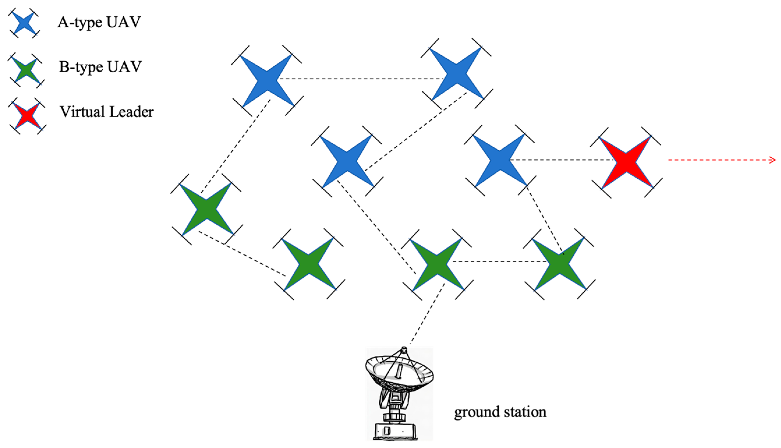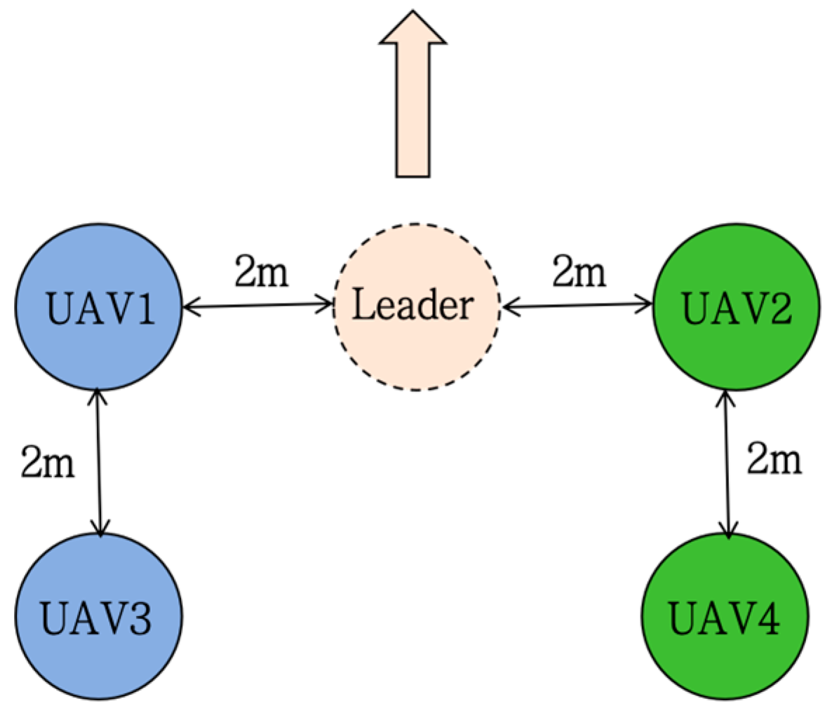Currently, the control algorithms for drone swarms mainly include behavior-based [6], virtual structure [7], and leader–follower [8] methods. The behavior-based approach controls the actions of each drone in the swarm independently, making it suitable for specific task scenarios. However, due to the lack of global coordination, ensuring the stability of the swarm is challenging. The virtual structure approach theoretically addresses this problem and guarantees swarm stability. However, since the formation is pre-defined and its ability to avoid obstacles in dynamic environments is limited, it lacks flexibility. In contrast, the leader–follower approach combines the benefits of both, offering a simple model, strong stability, and good adaptability, which has led to its widespread application in practice. Therefore, the formation control method adopted in this paper is the leader–follower method.

To ensure stable formation flight, the trajectory planning of multi-drone systems has been a key area of research. In an unknown environment, a drone cannot pre-plan its trajectory before movement because it has not built a model of the surrounding area in advance. Therefore, it can only continuously plan its next movement trajectory in real time based on environmental information obtained from sensors during movement. Since the planning is performed online in real time, trajectory planning and execution are closely linked. The planned path must satisfy the drone’s kinematics and dynamics during the planning process to ensure that the trajectory is tracked and executed in a timely manner. This places high demands on both the speed of trajectory generation and the quality of the trajectory. Additionally, due to the unpredictability of the environment and frequent unexpected changes, it is required that the robot can quickly alter its trajectory and perform re-planning promptly to avoid collisions with obstacles. Mainstream planning algorithms include graph-search-based methods [9,10], artificial potential field methods [11,12], metaheuristic algorithms [13,14], and optimal control algorithms such as model-based control [15,16]. John Bellingham et al. [17], in their study of fixed-wing trajectory optimization, transformed the problem into a mixed-integer linear programming problem to optimize the shortest time path to the target point. Y. You et al. [18] proposed a hybrid algorithm based on an improved A* algorithm and multi-objective artificial potential field (MTAPF) for leader–follower formation planning in static environments. Michael Watterson et al. [19] proposed a method that combines a short-term receding horizon control (RHC) strategy and long-term receding horizon control strategy, based on the theory of receding horizon control. After using the Delaunay method to convexify the environment, they constructed a quadratic programming problem within it to complete the real-time trajectory generation process. L. Chang et al. [20] addressed the challenge of real-time obstacle avoidance and maintaining formation flight in complex environments, proposing a combined leader–follower and behavior-based control algorithm using the improved dynamic window approach (DWA). G.Y. Cong et al. [21] used an improved RRT algorithm and 4D coordination cost function to plan global paths for each drone, with a heuristic artificial potential field (HAPF) algorithm for local collision avoidance, enabling 4D collaborative path planning for all drones. Although these methods can theoretically avoid obstacles, they often fail to consider trajectory tracking performance, which may lead to drones failing to precisely follow planned paths in actual flight, potentially causing collisions or failure to maintain formation. To address this issue, simplified UAV models and state constraints are often considered during the trajectory planning phase. Daniel Mellinger and Vijay Kumar [22] first proposed the Minimum Snap trajectory planning algorithm, which leverages the differential flatness property of rotary-wing drones. This algorithm can estimate polynomial trajectories and generate the optimal trajectory in real time. By formulating and solving a quadratic programming problem, it ensures safe passage through designated corridors while satisfying constraints on velocity, acceleration, and control inputs. Arul SH [23] combined trajectory planning with Model Predictive Control (MPC) to propose a distributed multi-UAV trajectory planning method that satisfies dynamic constraints, enabling real-time path planning for collision avoidance. M.Q.Cheng et al. [24] presented a state-constrained cooperative co-evolutionary algorithm (CCEA-ADVS) that improves computational efficiency, convergence speed, and path planning performance through an adaptive decision variable selection strategy and two-phase evolutionary optimization process. J. Wu et al. [25] added simple constraints such as air resistance and thrust to a kinematic model. P. Yao et al. [26] employed a trajectory propagation approach to iteratively solve the dynamics equations of the vehicle, considering both the planned path and the constraints of UAV dynamics. While these methods account for some dynamic constraints, they still have significant gaps with real flight constraints and fail to adequately consider controller performance, leaving doubts about accurate path tracking in practice. Moreover, applying the same constraints to all drones limits their applicability in heterogeneous UAV formations. Y. Lin et al. [27] combined vehicle models with controllers to simulate the vehicles’ trajectories using elementary control signals. L.Y. Heng et al. [28] integrated low-level controllers with a UAV’s six-dimensional nonlinear motion model to predict flight trajectories during the planning phase. Inspired by these approaches, in the process of trajectory planning, the dynamics model of a quadcopter can be integrated with tracking control algorithms to forecast real flight paths. The artificial potential field method is computationally simple, is easy to implement, and offers good real-time performance, enabling it to quickly respond to environmental changes. It is particularly suitable for real-time navigation in dynamic environments. Furthermore, the algorithm’s parameters are relatively intuitive to adjust, allowing for flexible optimization based on different task requirements. By constructing a cost function based on the predicted actual flight trajectory and using particle swarm optimization, the optimal parameters for the artificial potential field method can be found, enabling the drone to track the planned trajectory as accurately as possible during actual flight. Additionally, for heterogeneous UAV formations, trajectory prediction can be based on the dynamics models and control algorithms of each UAV, allowing for tailored flight trajectory planning.

However, the quadcopter model is represented by a set of interconnected nonlinear differential equations [29], and each step requires integration, resulting in low planning efficiency. At the same time, the accuracy of the prediction relies significantly on the precision and accuracy of the quadcopter model. Therefore, using this model for prediction is both time-consuming and difficult to ensure sufficient accuracy with. As computer technology and artificial intelligence continue to evolve, deep learning is increasingly being adopted across various industries. Significant achievements have been made in fields such as image processing, machine translation, speech recognition, and human–computer games [30,31,32,33]. Motivated by the benefits of deep learning, we investigated its potential to address the trajectory prediction challenge. In fact, drone trajectory prediction can be viewed as a mapping between control signals produced by the control system and the resulting flight path, which fundamentally represents a time series forecasting problem. Data-driven methods can not only effectively capture this mapping relationship but also significantly reduce the complexity of modeling. H. Ping et al. [34] used LSTM to predict 4D motion trajectories. W. Ru [35] proposed a multi-information fusion Convolutional Neural Network (MI-CNN) based on attention mechanisms to predict pedestrian trajectories. X. Gou et al. [36] proposed a vehicle trajectory prediction model combining CNN and LSTM neural networks. CNN networks are adept at handling spatial information and can effectively extract spatial features from trajectory data, while LSTM networks possess long-term and short-term memory capabilities, making them suitable for processing time series data. By combining the strengths of CNNs and LSTM, the spatiotemporal features of the data can be fully leveraged.

Inspired by the above analysis and research, this paper proposes a real-time trajectory planning method for heterogeneous UAV formations based on a CNN-LSTM trajectory prediction network with a focus on control. The main contributions of this paper are summarized as follows:

• To fully consider the tracking characteristics and ensure that the heterogeneous UAV formation can maintain formation flight during the flight process, we combine the UAV model with the control system to predict the actual flight trajectory of the formation during the trajectory planning phase.
• To reduce the complexity of quadcopter modeling and improve the trajectory planning efficiency, we use the CNN-LSTM network to replace traditional physical models. The actual flight trajectory of the UAV is predicted based on the control signals generated by the control system.
• A framework for real-time trajectory planning of heterogeneous UAV formations is designed, where CNN-LSTM prediction networks for different types of UAVs are pre-trained. Drawing on the idea of Model Predictive Control (MPC), during the planning phase, an improved artificial potential field (APF) method is used to plan multi-step trajectory points. The planning cost is evaluated by predicting the formation’s flight trajectory using the CNN-LSTM network, and optimization is performed using a multi-objective particle swarm optimization algorithm (MOPSO). In the actual flight phase, based on the optimized parameters, the improved APF method is used again to plan multi-step trajectory points, and the formation follows the trajectory points for flight.

The rest of this paper is organized as follows: Section 2 establishes the dynamics model of the quadcopter formation and describes the formation tracking control scheme. Section 3 gives a comprehensive overview of the control-oriented UAV formation trajectory planning method. Section 4 presents simulation, comparison, and analysis results. Section 5 concludes this paper.

2. Quadcopter Formation Control System Model

This section provides a detailed introduction to the dynamics model of the quadrotor UAV and the trajectory tracking control scheme based on sliding mode control and a neural network observer.

2.1. Quadcopter Dynamics Model

In the scenario where a specific task needs to be performed, multiple types of quadcopters are required to collaborate with each other. During this process, the drones must fly in formation based on the signals from a virtual leader in order to successfully reach the task position, as shown in Figure 1.

Each drone has different aerodynamic parameters, body dimensions, and physical characteristics such as moment of inertia. the dynamic equation of the kth quadcopter (k = 1, 2, …, N) can be described as

$$\left\{\begin{array}{l}{\ddot{x}}_k=u_{x,k}-K_{1,k}{\dot{x}}_k/m_k\\ {\ddot{y}}_k=u_{y,k}-K_{2,k}{\dot{y}}_k/m_k\\ {\ddot{z}}_k=u_{z,k}-K_{3,k}{\dot{z}}_k/m_k-g\\ {\ddot{\varphi }}_k=U_{2,k}-l_k^{*}{K}_{4,k}{\dot{\varphi }}_k/I_{x,k}+(I_{y,k}-I_{z,k}){\dot{\theta }}_k{\dot{\phi }}_k/I_{x,k}\\ \hspace{1em}\hspace{1em}+J_k{\dot{\theta }}_k{\Omega }_k/I_{x,k}\\ {\ddot{\theta }}_k=U_{3,k}-l_k^{*}{K}_{5,k}{\dot{\theta }}_k/I_{y,k}+(I_{z,k}-I_{x,k}){\dot{\varphi }}_k{\dot{\phi }}_k/I_{y,k}\\ +J_k{\dot{\varphi }}_k{\Omega }_k/I_{y,k}\\ {\ddot{\phi }}_k=U_{4,k}-l_k^{*}{K}_{6,k}{\dot{\phi }}_k/I_{z,k}+(I_{x,k}-I_{y,k}){\dot{\varphi }}_k{\dot{\theta }}_k/I_{z,k}\end{array}\right.$$

(1)

where N represents the number of quadcopters in the formation; $[x_k,y_k,z_k]$ are the kth drone’s center of mass position coordinates in the inertial reference frame; $[{\varphi }_k,{\theta }_k,{\phi }_k]$ represent three attitude angles (roll, pitch, yaw) of the kth drone; $m_k$ represents the total mass of the drone; g represents the acceleration due to gravity; $K_{j,k}$ (j = 1, 2, …, 6) are the corresponding air drag coefficients; $l_k^{*}$ is the distance from the propeller axis to the drone’s center of mass; $[I_{x,k},I_{y,k},I_{z,k}]$ are the moment of inertia of the drone’s body along the three axes in the body-fixed coordinate system; $J_k$ is the moment of inertia of the propeller; ${\Omega }_k$ is the deviation of the propeller’s rotational speed; and $[u_{x,k},u_{y,k},u_{z,k}]$ are the virtual control inputs, defined as

$$\left\{\begin{array}{l}{u}_{x,k}=(\sin {\varphi }_k\cos {\theta }_k\cos {\phi }_k+\sin {\theta }_k\sin {\phi }_k)U_{1,k}\\ u_{y,k}=(\sin {\varphi }_k\cos {\theta }_k\sin {\phi }_k-\sin {\theta }_k\cos {\phi }_k)U_{1,k}\\ u_{z,k}=(\cos {\varphi }_k\cos {\theta }_k)U_{1,k}\end{array}\right.$$

(2)

where $[U_{1,k},U_{2,k},U_{3,k},U_{4,k}]$ represent control inputs produced by the four propeller motors, defined as

$$\left\{\begin{array}{l}{U}_{1,k}=b_k({\omega }_{1,k}^2+{\omega }_{2,k}^2+{\omega }_{3,k}^2+{\omega }_{4,k}^2)/m_k\\ U_{2,k}=l_k^{*}{b}_k({\omega }_{4,k}^2-{\omega }_{2,k}^2)/I_{x,k}\\ U_{3,k}=l_k^{*}{b}_k({\omega }_{3,k}^2-{\omega }_{1,k}^2)/I_{y,k}\\ U_{4,k}=C({\omega }_{1,k}^2-{\omega }_{2,k}^2+{\omega }_{3,k}^2-{\omega }_{4,k}^2)/I_{z,k}\end{array}\right.$$

(3)

where $b_k$ is the lift coefficient of the propeller; C is the torque coefficient; and $[{\omega }_{1,k},{\omega }_{2,k},{\omega }_{3,k},{\omega }_{4,k}]$ are the rotational speeds of four propellers.

2.2. Quadcopter Formation Tracking Control Scheme

The control scheme for formation tracking in this paper is shown in Figure 2. First, the kth drone acquires the virtual leader signal from the ground station through a communication network, which provides the desired position $[x_k^o,y_k^o,z_k^o]$ and desired yaw angle ${\phi }_k^o$. The desired position coordinates are used by a position assistance controller to generate virtual control inputs $[u_{x,k},u_{y,k},u_{z,k}]$, from which the desired thrust $U_{1,k}$ is calculated. Additionally, the desired roll and pitch angle $[{\varphi }_k^o,{\theta }_k^o]$ are obtained, and the corresponding desired torque $[U_{2,k},U_{3,k},U_{4,k}]$ is computed by combining the desired yaw angle through the attitude controller. To ensure the robustness of the system, both controllers adopt a sliding mode control strategy, and disturbance observers based on a radial basis function (RBF) neural network are introduced to compensate for external disturbances. Finally, by combining the desired thrust and torque, the desired rotational speeds $[{\omega }_{1,k}^o,{\omega }_{2,k}^o,{\omega }_{3,k}^o,{\omega }_{4,k}^o]$ for the four propellers are calculated. Since the focus of this paper is not on the detailed elaboration of the drone formation control strategy, the specific content and stability analysis of the control scheme can be found in reference [37].

Assumption 1. 

The quadrotor UAVs in the formation are able to maintain communication with the ground station, transmitting their own state information in real time and receiving signals from the virtual leader.

After obtaining the desired rotational speeds for the four propellers, the throttle command is calculated by the motor controller as the final control signal. In the simulation, the relationship between the motor speed and the throttle command is assumed to be linear:

$${\sigma }_{i,k}={\displaystyle \frac{1}{C_{R,k}}}({\omega }_{i,k}^o-{\omega }_{b,k})$$

(4)

$${\omega }_{i,k}=C_{R,k}{\sigma }_{i,k}+{\omega }_{b,k}$$

(5)

where $C_R,{\omega }_b$ are the parameters of the motor.

Remark 1. 

In the simulation, for simplicity, it is approximated that the relationship between the motor speed and the throttle command is linear. In the actual system, the relationship between them is complex and nonlinear, which is one of the reasons for using data-driven deep neural networks to predict flight trajectories.

3. Control-Oriented Trajectory Planning Method for UAV Formation

This section provides a detailed introduction to the trajectory planning scheme for heterogeneous UAV swarm formation. It mainly includes the overall framework, the improved artificial potential field method, and the CNN-LSTM-based trajectory prediction scheme and cost function, as well as the multi-objective particle swarm optimization algorithm.

3.1. Overall Framework

The framework for planning the trajectory points of a heterogeneous UAV formation, introduced in this paper, is depicted in Figure 3. The framework consists of four main modules: the artificial potential field (APF) module, the sliding mode control (SMC) module, the CNN-LSTM flight trajectory prediction module, and the multi-objective optimization (MOPSO) module. The APF module generates target trajectory points $[x^{o^{\prime }},y^{o^{\prime }},z^{o^{\prime }}]$ based on the positions of the target points and surrounding obstacles. The kth UAV calculates its target trajectory points $[x_k^{o^{\prime }},y_k^{o^{\prime }},z_k^{o^{\prime }}]$ based on its relative position within the formation and compares it with the current actual flight state, and the throttle command $[{\sigma }_{1,k}^{\prime },{\sigma }_{2,k}^{\prime },{\sigma }_{3,k}^{\prime },{\sigma }_{4,k}^{\prime }]$ is obtained from the Motor Allocation using the sliding mode control method shown in Figure 2. The CNN-LSTM module, as the flight trajectory prediction module, predicts the flight state at the next time step by combining historical flight state information and the current throttle command.

After the flight trajectory predictions for all UAVs are completed, four cost functions are evaluated based on these trajectories. The MOPSO algorithm is then used to optimize these four cost functions, obtaining the step size and repulsive coefficient corresponding to the minimum cost. These two parameters are used as the actual control values for generating the virtual leader signal, which is applied in the leader-following system. The UAVs in the formation track the trajectory based on this signal and update their flight states. Subsequently, the trajectory planning module will plan the next trajectory step based on the new states. This process repeats iteratively, ultimately producing the complete target trajectory and the actual flight trajectory.

By comprehensively considering the UAVs’ trajectory tracking capabilities and formation-keeping performance during the planning phase, the actual flight trajectory of the UAV formation is ultimately able to accurately track the target trajectory while maintaining a stable formation throughout the flight.

Remark 2. 

The UAV executes control every 1 millisecond, while the communication cycle with the ground station is 100 milliseconds, meaning that the flight trajectory needs to be planned for 100 time steps each time.

Remark 3. 

To increase the stability and controllability of UAV flight, the target and actual trajectories are treated as two separate and independent trajectories.

Remark 4. 

Due to experimental limitations, it is not possible to collect a large amount of real-world UAV flight data for training the neural network. Therefore, simulation data with added disturbances is used as a substitute.

Further analysis is conducted on the errors generated during the entire planning process. The first error E₁ is the difference between the simulated flight trajectory L₁ and the actual flight trajectory L₂ in the real system. The second error E₂ is the difference between the predicted actual trajectory L₃ and the simulated trajectory L₁. The total error E₃ is the difference between the predicted actual trajectory L₃ and the actual flight trajectory L₂ in the real system. The formula is as follows:

$$E_1=L_1-L_2$$

(6)

$$E_2=L_3-L_1$$

(7)

$$E_3=E_2+E_1=L_3-L_2$$

(8)

where E₂ represents the prediction capability of the network, which can be reduced by properly designing the network structure and parameters. On the other hand, E₁ reflects the accuracy of the UAV modeling, and this deviation is difficult to avoid. This is the reason for using a data-driven neural network approach to predict trajectories. If experimental conditions allow and a large amount of real flight data can be collected, the total error E₃ would be equal to E₂, thereby meeting the required experimental accuracy.

3.2. Improved Artificial Potential Field Method

To apply the APF method in a complex 3D environment, a grid-based approach is used to model the map. During the UAV’s flight, It can continuously monitor the surrounding grids in real time and determine if there are any obstacles. The detection results are used to calculate the shortest distance between the current position and the grid as input for subsequent algorithm computations, enabling effective trajectory planning and obstacle avoidance.

The gravitational force (F_att) formula is as follows:

$$F_{att}=k_{att}\rho (q,q_t)$$

(9)

where k_att is the gravitational coefficient and $\rho (q,q_t)$ is the distance between the UAV’s position q and the target position q_t.

When there are obstacles near the target position, the UAV may oscillate and hover around the target position without being able to reach it. To address this issue, the relative distance between the UAV and the target position is introduced into the repulsive potential field. The repulsive force (F_rep) formula is as follows:

$$F_{rep}=\left\{\begin{array}{ll}{F}_{rep1}+F_{rep2}& \rho (q,q_{ob})\le {\rho }_0\\ 0& else\end{array}\right.$$

(10)

$$\begin{array}{l}{F}_{rep1}=k_{rep}(1/\rho (q,q_{ob})-1/{\rho }_0){\rho }^n(q,q_t)\\ /{\rho }^2(q,q_{ob})\end{array}$$

(11)

$$F_{rep2}=n{k}_{rep}{(1/\rho (q,q_{ob})-1/{\rho }_0)}^2{\rho }^{n-1}(q,q_t)/2$$

(12)

where k_rep is the repulsive coefficient; $\rho (q,q_{ob})$ is the Euclidean distance between the UAV’s position q and the obstacle’s position q_ob; and ${\rho }_0$ is the repulsive influence range.

When the magnitudes of the repulsive and gravitational forces are equal and their directions are opposite, a local minimum may occur, causing the UAV to oscillate at that position. To break out of this equilibrium state, a control force can be introduced to disrupt the force balance. The condition for detecting such an equilibrium state is as follows:

$$\left\{\begin{array}{l}\pi -{\theta }_0\le {\epsilon }_1\\ |F_{rep}-F_{att}|\le {\epsilon }_2\end{array}\right.$$

(13)

where ${\theta }_0$ is the angle between the resultant repulsive force from all obstacles and the gravitational force and ${\epsilon }_1,{\epsilon }_2$ are close to small values near 0.

The formula for the control force (F_d) is

$$F_d=F_{req}^{\prime }+\mu F_{att}$$

(14)

The direction of $F_{req}^{\prime }$ is perpendicular to the resultant repulsive force from all obstacles, and its value is equal to that of the resultant repulsive force; $\mu$ is the control coefficient.

The magnitude of the total force acting on the UAV in the potential field is

$$F=F_{req}+F_{att}+F_d$$

(15)

The displacement vector of the drone in one time step is

$$\Delta =\Delta rF$$

(16)

where $\Delta r$ is the step size.

The three key parameters of the artificial potential field method are the gravitational coefficient, repulsion coefficient, and step size. The gravitational and repulsion coefficients work together to enable real-time obstacle avoidance for the UAV, while the step size is used to adjust the UAV’s movement speed and tracking accuracy. By fixing the gravitational coefficient and optimizing the repulsion coefficient and step size, the obstacle avoidance effect can be ensured while improving the flight speed and formation stability of the drone swarm.

3.3. Trajectory Prediction Network

Drone models often struggle to fully account for unmodeled dynamics and unknown disturbances, leading to significant deviations in flight trajectory predictions due to inaccurate models. In contrast, data-driven methods based on neural networks can effectively improve prediction accuracy. CNNs (Convolutional Neural Networks) excel at processing spatial information and can efficiently extract spatial features from trajectory data, while LSTM (Long Short-Term Memory networks) possess memory capabilities that make them suitable for handling time-series data. The CNN-LSTM trajectory prediction model is introduced by integrating the advantages of CNNs and LSTM, with the aim of establishing a mapping relationship between the control signals output by the control system and the UAV’s flight trajectory. The network uses the UAV’s historical flight states and current throttle commands to predict future flight trajectories.

The design of the proposed CNN-LSTM trajectory prediction model is presented in Figure 4. First, the UAV’s position and attitude information from the past 10 time steps is integrated as the network input. Then, two identical 1D convolutional layers are used to extract the spatial features from the input data. The resulting feature maps are then passed to the LSTM network to capture the temporal features. Finally, the output from the LSTM network is concatenated with the UAV’s current throttle command and passed through a fully connected layer to produce the final prediction result.

The input to the CNN-LSTM network consists of historical flight state information and the current throttle command:

$$u_t=[x,y,z,\varphi ,\theta ,\phi ]$$

(17)

$$U_t=[u_{t-9},u_{t-8},\cdots ,u_{t-1},u_t]$$

(18)

$$v_t=[{\sigma }_1,{\sigma }_2,{\sigma }_3,{\sigma }_4]$$

(19)

where u_t represents the current flight state of the UAV; U_t is the flight data of the UAV from the past 10 time steps, which serves as the input to the convolutional network; and v_t is the current throttle command of the UAV, which is part of the input data to the fully connected layer.

The output of the CNN-LSTM network is the predicted flight state for the next time step:

$${\widehat{y}}_t=[x,y,z,\varphi ,\theta ,\phi ]$$

(20)

The specific parameters of the trajectory prediction model are shown in

Table 1. CNN-LSTM model parameters.

Layer Definition	Layer Parameters	Layer Definition
1D Conv1	neurons: 50, length: 3	1D Conv1
1D Conv2	neurons: 50, length: 3	1D Conv2
LSTM1	neurons: 50	LSTM1
LSTM2	neurons: 50	LSTM2
Dropout1	dropout: 0.2	Dropout1
FC1	neurons: 50	FC1
FC2	neurons: 50	FC2

. The model is composed of two convolutional layers, two LSTM layers, and two fully connected layers. To prevent overfitting, a dropout layer is added before the fully connected layers to enhance the model’s generalization ability.

Remark 5. 

Due to the strong time-series prediction capability of LSTM, the CNN-LSTM model can not only predict the flight state at the next time step but also predict the flight states for multiple future time steps by progressively accumulating the predicted states. This characteristic enables the model to anticipate formation trajectories further into the future, providing more stable support for trajectory tracking, real-time obstacle avoidance, and formation maintenance.

3.4. Cost Function

This paper next focuses on designing the cost function based on three key performance factors, trajectory tracking, formation maintenance, and real-time obstacle avoidance, in order to ensure the feasibility of waypoint planning and the stability of formation flight.

First, to ensure that the drone swarm can maintain stable formation flight, it is essential to focus on the relative positions between the drones. Therefore, a constraint based on the distance between drones is designed, which not only effectively improves the formation maintenance capability but also reduces the risk of collisions between drones. The cost function J₁ is designed as follows:

$$J_1={\displaystyle \sum _{i=1}^{100}{\displaystyle \sum _{j=1}^N\left|\rho (P_{i,j},P_{i,j+1})-d_j\right|}}$$

(21)

where P_ij denotes the actual position of the jth drone at the ith time step; $\rho (P_{i,j},P_{i,j+1})$ represents the distance between the jth drone and the j + 1th drone at the ith time step; and d_j denotes the fixed distance that should be maintained between the jth and j + 1th drones.

In formation flight, maintaining accurate tracking of the target trajectory is crucial. Therefore, a cost function J₂ is designed to measure the deviation between the target trajectory and the actual flight trajectory:

$$J_2={\displaystyle \sum _{i=1}^{100}{\displaystyle \sum _{j=1}^N\rho (P_{i,j},P_{i,j}^o)}}$$

(22)

where $P_{i,j}^o$ represents the target position that the jth drone needs to track at the ith time step.

In the formation flight process, the formation’s obstacle avoidance capability is equally important. In the APF module, we already used the grid method to model the environment. Therefore, when calculating the cost function J₃, this method can still be used to effectively evaluate the obstacle avoidance performance.

$$\begin{array}{l}ris{k}_{i,j,k}=\left\{\begin{array}{ll}{d}_0-d_{i,j,k}& d_{i,j,k}<d_0\\ 0& else\end{array}\right.\\ Ris{k}_{i,j}={\displaystyle \sum _{k=1}^{m}ris{k}_{i,j,k}}\\ J_3={\displaystyle \sum _{i=1}^{100}{\displaystyle \sum _{j=1}^{N}Ris{k}_{i,j}}}\end{array}$$

(23)

where d₀ represents the safety distance of the drone; d_i,j,k is the distance between the jth drone and the kth obstacle grid at the ith time step; and m represents the total number of obstacle grids surrounding the jth drone at the ith time step.

By using the distance between the current position of the drone and the final target point as a constraint, the flight speed can be appropriately increased while maintaining the stability of the formation. The cost function J₄ is designed as follows:

$$J_4={\displaystyle \sum _{j=1}^N\rho (P_{100,j},P_{T,j})}$$

(24)

where P_T,j is the final target position of the jth drone.

By using a multi-objective optimization algorithm to jointly optimize these four cost functions, the optimal artificial potential field parameters can be obtained. These optimized parameters can be used to generate virtual leader signals, allowing the formation to move at maximum speed while maintaining stability, real-time obstacle avoidance, and precise trajectory tracking, ultimately reaching the target position efficiently.

3.5. Multi-Objective Particle Swarm Optimization (MOPSO) Algorithm

The optimization objectives of this paper focus on the cost functions J₁, J₂, J₃, and J₄, which are designed around three key performances: trajectory tracking, formation keeping, and real-time obstacle avoidance. The decision variables are the step size and repulsive coefficient of the artificial potential field method. The standard form is presented as follows:

$$\begin{array}{ll}minimize& [J_1(\Delta r,RP),J_2(\Delta r,RP),J_3(\Delta r,RP),J_4(\Delta r,RP)]\\ subjectto& \Delta r\in R_1\\ & RP\in R_2\end{array}$$

(25)

where J₁, J₂, J₃, and J₄ are the cost functions; $\Delta r$ is the step size; RP is the repulsion coefficient; and R₁ and R₂ represent their constraint sets.

The overall process of the MOPSO algorithm is similar to that of the PSO algorithm. The main difference is that single-objective optimization problems typically have a clear optimal solution, while in multi-objective optimization problems, the objective functions are often in conflict with each other. As a result, it is not possible to have a single solution that minimizes all objective functions simultaneously. To address this issue, the concept of dominance is introduced.

Theorem 1. 

Let p and q be any two distinct individuals in the population. p is said to dominate q if the following two conditions are satisfied:

• For all sub-objectives, p is no worse than q.

  $$f_k(p)\le f_k(q)k=1,2\cdots r$$

  (26)
• There exists at least one sub-objective in which p is better than q.

$$\exists l\in \left\{1,2,\cdots ,r\right\},f_l(p)<f_l(q)$$

(27)

where r is the number of sub-objectives.

This dominance relationship defines the relative quality among multiple solutions and allows for the identification of a set of nondominated solutions in multi-objective optimization, known as the Pareto front.

The update process of the individual best position involves two scenarios: if the current solution dominates the historical best position, the current position is updated as the new individual best. If the current solution and the historical best position do not dominate each other, a new historical best is randomly selected from the solutions.

The global best position needs to be selected from the Pareto front. To find the sparsest point, the concept of crowding distance is introduced. Crowding distance is used to measure the distribution density of solutions on the Pareto front and is typically calculated as follows:

$$I(x_i)={\displaystyle \sum _{j=1}^4\left|J_j(x_m)-J_j(x_n)\right|/(J_{j,\max }-J_{j,\min })}$$

(28)

where x_m and x_n are the two particles closest to x_i; J_j(x_m) is the value of the jth objective function of particle x_m; and J_j,max and J_j,min are the maximum and minimum values of the jth objective function among all particles.

During each iteration, the solution with the greatest crowding distance on the Pareto front is chosen as the global best position. The particle’s velocity and position are then updated based on both the individual and global best positions, continuing until the termination condition is met. After the iteration ends, a solution is selected from the Pareto front as the optimal solution. When the velocity is low or the tracking performance is more favorable, priority should be given to improving the formation speed, whereas when the velocity is high, more focus should be placed on trajectory tracking and formation maintenance. Based on this requirement, an optimal solution selection function is designed:

$$J=\left\{\begin{array}{ll}{J}_1+J_3+J_4& v<5ordis<1\\ J_1+J_2+J_3& v>5\end{array}\right.$$

(29)

where v is the formation flight speed and dis is the average deviation between the actual trajectory of each UAV and the target trajectory.

The overall framework of MOPSO is shown in Algorithm 1.

Algorithm 1 MOPSO.

Input: maximum number of iterations T, population size N

1:   Initialize the positions and velocities of the population

2:   while (t < T):

3:  for i = 1 to N:

4:    Calculate the fitness function using Equations (21) to (24)

5:    Update the individual best position

6:    Update the Pareto front

7:  Calculate the crowding distance using Equation (27)

8:  Update the global best position

9:  Update the particles’s velocity and position

10: Select the optimal solutionaccording to Equation (28)

Output: step size, repulsive coefficient

4. Simulation and Analysis

To verify the feasibility of the proposed control-oriented heterogeneous UAV formation trajectory planning method, simulation calculations were performed on a desktop computer (AMD Ryzen 5 3500X 6-Core Processor @ 3.60 GHz, 16.0GB RAM, 1660 GPU) with a simulation step size of 0.001.

4.1. Performance Verification of CNN-LSTM Network

Based on the quadrotor UAV model and tracking control algorithm mentioned in the Section 2 of this paper, 50 trajectories were generated, resulting in a total of 2 million data points. The data format follows Equations (18) and (19), with 1.8 million data points used for training and 200,000 data points used for testing. To accelerate network training and achieve better convergence, the input data were standardized, that is,

$$u_n={\displaystyle \frac{u-u_{\min }}{u_{\max }-u_{\min }}}$$

(30)

where u_n is the normalized data sample; u is the original data sample; u_max is the maximum value in the sample; and u_min is the minimum value in the sample.

The CNN-LSTM trajectory prediction model’s performance is measured by Mean Squared Error (MSE). The formula for computing this evaluation metric is as follows:

$$MSE={\displaystyle \frac{1}{n}}{\displaystyle \sum _{i=1}^n{(y_i-{\widehat{y}}_i)}^2}$$

(31)

where n is the total number of samples; y_i is the actual value; and ${\widehat{y}}_i$ is the predicted value.

We assessed the prediction accuracy of the proposed CNN-LSTM network by comparing it with a Fully Connected Network (FC), a CNN, and an LSTM. The settings for each network’s parameters are detailed in

Table 2. Comparison of model architecture parameters.

Model	Layer Definition	Layer Parameters
LSTM	LSTM1	neurons: 50
	LSTM2	neurons: 50
	FC1	neurons: 50
	FC2	neurons: 50
	FC3	neurons: 50
CNN	1D Conv1	neurons: 50, Length: 3
	1D Conv1	neurons: 50, Length: 3
	FC1	neurons: 50
	FC2	neurons: 50
	FC3	neurons: 50
FC	FC1	neurons: 50
	FC2	neurons: 50
	FC3	neurons: 50
	FC4	neurons: 50
	FC5	neurons: 50

.

To ensure fairness in the comparison, the training parameters for all four models were kept consistent (200 training epochs, initial learning rate of 0.001, and batch size of 64). After training, we compared the four models on the test set, with the results shown in

Table 3. Comparison of different models on the test set.

	CNN-LSTM	LSTM	CNN	FC
MSE	6.36 × 10−6	7.03 × 10−6	7.44 × 10−6	9.65 × 10−6

. Compared to the other three models, the CNN-LSTM model has the smallest MSE. Specifically, both the LSTM and CNN models outperform the FC model in terms of MSE, indicating that the model’s prediction accuracy improves significantly after extracting spatial or temporal features. This further demonstrates the significant superiority of the CNN-LSTM model in prediction performance, which combines the advantages of both CNN and LSTM models.

The method for trajectory planning proposed in this paper relies on multi-step flight trajectory prediction. In the multi-step prediction process, the primary focus is on the accuracy of the trajectory. Therefore, the Mean Absolute Error (MAE) is used to calculate the trajectory error without considering the error in the attitude angles, as this approach better aligns with the practical requirements of real-world applications. To evaluate the performance of the proposed model in multi-step prediction, a complete trajectory was selected from the test set, and the multi-step prediction results of each model were calculated. The specific data are shown in

Table 4. Multi-step prediction results of different models.

Prediction Step	CNN-LSTM	LSTM	CNN	FC
1	1.93 × 10−8	4.33 × 10−8	3.89 × 10−8	7.87 × 10−7
5	2.78 × 10−7	6.76 × 10−7	6.06 × 10−7	1.12 × 10−5
10	1.02 × 10−6	2.52 × 10−6	2.15 × 10−6	3.89 × 10−5
50	2.13 × 10−5	6.59 × 10−5	4.58 × 10−5	8.21 × 10−4
100	7.31 × 10−5	2.97 × 10−4	1.78 × 10−4	2.98 × 10−3

. The results indicate that when the prediction horizon is short, the prediction errors of the four models are relatively similar. However, as the prediction horizon increases, the prediction errors of all models grow, and the differences in errors also gradually expand. At this point, the superiority of the proposed model becomes more apparent. The detailed results for predicting 100 steps are shown in Figure 5. The CNN-LSTM model significantly outperforms the other models in prediction accuracy, particularly in predicting the attitude angles, where the difference is especially noticeable. The average prediction error for the 100-step trajectory is less than 0.0001 m, fully meeting the accuracy requirements. Therefore, the CNN-LSTM trajectory prediction model is fully suitable for the proposed trajectory planning method.

To conduct a more thorough validation of the CNN-LSTM model’s performance in long-term prediction, we selected a segment of the target flight path planned using the proposed trajectory planning method. We used these four models to predict the actual flight trajectory over the next 10 s. The detailed final prediction results are shown in Figure 6. The results demonstrate that the CNN-LSTM model greatly exceeds the performance of the other models in terms of trajectory and attitude angle prediction accuracy. Especially when compared to the CNN and FC models, the CNN-LSTM model exhibits much smaller deviations in trajectory prediction. The specific trajectory deviation data are shown in

Table 5. Comparison of 10 s prediction results.

	CNN-LSTM	LSTM	CNN	FC
MAE (m)	0.3428	0.8513	2.1414	2.1791

, where the average trajectory errors for the CNN and FC models exceed 2 m, while the average errors for the CNN-LSTM and LSTM models are both less than 1 m, with CNN-LSTM achieving an error as small as 0.3428 m. This fully demonstrates the superiority of the CNN-LSTM model in long-term prediction and provides strong support for subsequent research and applications based on long-term predictions.

4.2. Formation Trajectory Planning Performance Verification

To verify the feasibility of the proposed trajectory planning method, the flight path of a formation of four quadrotor UAVs (i = {1, 2, 3, 4}) is planned as an example. The formation layout is shown in Figure 7. UAV1 and UAV3 are of the same model of quadrotor UAV, while UAV2 and UAV4 are of another model.

The UAV parameters for UAV1 and UAV3 are as follows:

m = 1.02 kg, l^* = 0.23 m, g = 9.8 m/s², I_x = I_y = 0.0075 kg·m, I_z = 0.013 kg·m, J = 6 × 10⁻⁵, K₁ = K₂ = K₃

=0.01 kg/m, K₄ = K₅ = K₆ = 0.012 kg/m, b = 6 × 10⁻⁵, C = 7.5 × 10⁻⁷.

The UAV parameters for UAV2 and UAV4 are as follows:

m = 1.4 kg, l^* = 0.225 m, g = 9.8 m/s², I_x = I_y = 0.0211 kg·m, I_z = 0.0366 kg·m, J = 1.287 × 10⁻⁴, K₁ = K₂

=K₃ = 0.01 kg/m, K₄ = K₅ = K₆ = 0.012 kg/m, b = 1.105 × 10⁻⁵, C = 1.779 × 10⁻⁷.

For these two types of UAVs, the trajectory prediction CNN-LSTM models for each are trained separately, named Net1 and Net2. These models are incorporated into the trajectory planning method proposed in this paper as the trajectory prediction module. The specific process of trajectory planning is shown in Algorithm 2.

Algorithm 2 Control-oriented trajectory planning method for UAV formation.

Input: Initial position, Target position, Net1, Net2, the range of $\Delta r,RP$

1: while not reach Target position:

2:    MOPSO:

3:    for i = 1 to 100:

4:   Generating target trajectory points based on $\Delta r,RP$ (16)

5:   Obtaining control inputs for four UAVs based on control (5)

6:   Using Net1 to predict the trajectories of UAV1 and UAV3

7:   Using Net2 to predict the trajectories of UAV2 and UAV4

8:    Calculating the cost function (21)–(24)

9:    Optimizing the parameters using the MOPSO algorithm

10:  Obtaining the optimal parameters $\Delta r,RP$ (28)

11:  for i = 1 to 100:

12:  Generating actual target trajectory points based on $\Delta r,RP$ (16)

13:  Obtaining control inputs for four UAVs based on control (5)

14:  Updating the positions and attitudes of four UAVs (1)

Output: Planned flight path

In a 200 × 200 × 200 map, multiple cylindrical obstacles are set. The initial position of the virtual leader is [0, 0, 0], and the initial positions of the four UAVs are [−2, 0, 0], [2, 0, 0], [−2, −2, 0], and [2, −2, 0], respectively. The UAVs maintain this formation for subsequent formation flying. The target position is [175, 175, 50], the yaw angle is always 0, the step size $\Delta r$ range is [0.001, 0.01], and the repulsive coefficient RP range is [10, 100], while the gravitational coefficient is fixed at 1. The results of the trajectory planning algorithm introduced in this paper are illustrated in Figure 8. The cost functions in the figure are averaged. Since UAV1 and UAV3 are of the same type and have identical target trajectories in the x and y directions, their flight paths overlap completely in these directions. Similarly, the flight paths of UAV2 and UAV4 exhibit the same characteristics. From the figure, it can be observed that the four UAVs are able to maintain formation during flight, successfully avoid obstacles, and achieve good trajectory tracking performance. Although the tracking performance is slightly insufficient at 25 s, the four UAVs are still able to maintain formation flight, quickly adjust their states, and realign with the subsequent trajectory. This demonstrates that the proposed trajectory planning method can effectively accomplish tasks such as trajectory tracking, real-time obstacle avoidance, and formation maintenance.

To further validate the performance of the proposed trajectory planning method, three sets of control experiments are designed. The first method uses only the APF method for trajectory planning, with a step size $\Delta r$ set to 0.01 and the repulsive coefficient RP set to 20. The second method also uses the APF method for trajectory planning, but the step size $\Delta r$ is set to 0.005, while the repulsive coefficient RP remains at 20. The third method simplifies the UAVs to mass point models and replaces the complex UAV dynamics and control models with simple constraints. This method’s artificial potential field and multi-objective optimization process are the same as the method proposed in this paper. The acceleration range in each direction is [−5, 5] and the velocity range is [−10, 10], consistent with the constraints in the control model. The trajectories planned by the first and third methods are shown in Figure 9. From the figure, it can be observed that the formation maintenance and trajectory tracking performance of the UAV formation tracking the trajectories planned by these two methods are poor. Furthermore, UAV2 and UAV4 in the first method failed to reach the target position. Although the third method reached the target position, it collided with an obstacle during flight.

The specific data for these three methods are shown in

Table 6. Comparison results of the four methods.

	Proposed	1	2	3
Total distance (m)	281.58	282.04	274.92	295.35
Flight time (s)	33.4	27.25	54.49	29.4
Speed (m/s)	8.43	10.35	5.04	10.05
Tracking error (m)	0.72	6.71	0.29	5.42
Formation stability	89.39%	49.88%	100%	44.93
Calculation time (s)	175	31	45	120
Reach target	True	False	True	True
Obstacle avoidance	True	True	True	False

. The total flight distance, speed, and tracking error are the average values for the four UAVs. Since UAV1 and UAV3 are of the same type, the distance between these two UAVs remains constant, and similarly, the distance between UAV2 and UAV4 remains constant. Therefore, we only focus on the distance between UAV1 and UAV2. As long as the distance deviation between these two UAVs does not exceed 0.5 m, it is considered that the formation is maintained in a flight state. When the step size is 0.005, the flight speed is the slowest, but the total flight distance, speed, tracking error, and formation maintenance rate are all optimal. However, the total time is 1.6 times that of the proposed method, making it unsuitable for time-sensitive flight tasks. When the step size is 0.01, the flight speed is the fastest, but the tracking error is much larger, nearly 10 times that of the proposed method, and the formation maintenance rate is below 50%, with the target position ultimately not reached. The method based on the mass point model with simple constraints caused a collision with an obstacle during flight, resulting in poor tracking error and formation maintenance. The method in this paper, however, comprehensively considers formation maintenance, trajectory tracking, and real-time obstacle avoidance. With a formation maintenance rate close to 90%, it successfully avoids obstacles and reaches the target position. Meanwhile, the flight speed is maximized while completing the task, with an average speed of 8.43 m/s, which essentially meets the task requirements.

However, in terms of computational efficiency, the trajectory planning method proposed in this paper performs the worst, with a computation time of 175 s, which does not meet the real-time requirements. The main reasons are threefold. First, after rasterizing the map, the computation of obstacle distances is very large. Second, the multi-objective particle swarm optimization process takes a long time. Third, the computing power of the computer is relatively weak. Future work will focus on improving the first two aspects. At the same time, the trajectory planning method proposed in this paper is computed by the ground station. As long as the ground station has sufficient computing power, it should meet the real-time requirements. Computational efficiency also limits the application of larger-scale drone formations and more complex environments. The more complex the environment and the more obstacles there are, especially if they are unevenly distributed, the more time it will take to compute obstacle distances. Similarly, as the drone scale increases, more obstacle distances need to be computed, and the calculation scale of the four cost functions becomes larger, which results in a longer optimization time. However, the overall trajectory planning framework is sound. As long as the calculation of optimized obstacle distances and the multi-objective optimization process are improved and computing power is enhanced, this trajectory planning method will be fully applicable to larger-scale drone formations and more complex geographical environments.

5. Conclusions

This paper investigates the real-time trajectory planning problem for heterogeneous UAV formations. Drawing on the principles of Model Predictive Control (MPC), we use an improved artificial potential field (APF) method to generate multi-step target trajectory points during the trajectory planning phase and predict the actual flight trajectory of the formation using a pre-trained CNN-LSTM network. Based on this, a multi-objective particle swarm optimization (MOPSO) algorithm is used to optimize four cost functions. In the actual flight phase, the optimized parameters are used to generate future multi-step trajectory points, which serve as virtual leader signals for the UAV formation to track and maintain formation flying. This paper compares the performance of the CNN-LSTM network with that of CNN, LSTM, and FC networks. The results show that the CNN-LSTM network ranks first in both short-term and long-term prediction accuracy, with the accuracy gap becoming more pronounced as the prediction horizon increases. Furthermore, we compare the proposed trajectory planning method with fixed-step artificial potential field trajectory planning and the mass point model trajectory planning method based on state constraints. Experimental results indicate that the proposed method has significant advantages in formation maintenance, trajectory tracking, and real-time obstacle avoidance performance. It can maintain high-speed flight while ensuring good flight stability and safety. These results fully demonstrate the high feasibility and practical application value of the proposed trajectory planning method. Currently, the obstacles considered in this study are static. Future research will extend to trajectory prediction and real-time obstacle avoidance for dynamic obstacles, as well as the improvement of computational efficiency, in order to further enhance the system’s adaptability and robustness in complex environments.

References

1. Cao, Y.; Cheng, X.; Mu, J. Concentrated coverage path planning algorithm of UAV formation tor aerial photography. IEEE Sens. J. 2022, 22, 11098–11111. [Google Scholar] [CrossRef]
2. Wang, Y.B.; Bai, P.; Liang, X.; Wang, W.; Zhang, J.; Fu, Q. Reconnaissance mission conducted by UAV swarms based on distributed PSO path planning algorithms. IEEE Access 2019, 7, 105086–105099. [Google Scholar] [CrossRef]
3. Hu, C.F.; Zhang, Z.L.; Yang, N.; Shin, H.S.; Tsourdos, A. Fuzzy multiobjective cooperative surveillance of multiple UAVs based on distributed predictive control for unknown ground moving target in urban environment. Aerosp. Sci. Technol. 2019, 84, 329–338. [Google Scholar] [CrossRef]
4. Shirani, B.; Najafi, M.; Izadi, I. Cooperative load transportation using multiple UAVs. Aerosp. Sci. Technol. 2019, 84, 158–169. [Google Scholar] [CrossRef]
5. Li, P.; Duan, H.B. A potential game approach to multiple UAV cooperative search and surveillance. Aerosp. Sci. Technol. 2017, 68, 403–415. [Google Scholar] [CrossRef]
6. El-Ferik, S. Biologically based control of a fleet of unmanned aerial vehicles facing multiple threats. IEEE Access 2020, 8, 107146–107160. [Google Scholar] [CrossRef]
7. Zhang, L.; Wang, J.; Lin, Z.; Lin, L.; Chen, Y.; He, B. Distributed Cooperative Obstacle Avoidance for Mobile Robots Using Independent Virtual Center Points. J. Intell. Robot. Syst. 2020, 98, 791–805. [Google Scholar] [CrossRef]
8. Zhang, Y.; Chen, J.; Chen, M.; Chen, C.; Zhang, Z.; Deng, X. Integrated the Artificial Potential Field with the Leader–Follower Approach for Unmanned Aerial Vehicles Cooperative Obstacle Avoidance. Mathematics 2024, 12, 954. [Google Scholar] [CrossRef]
9. Fransen, K.J.C.; van Eekelen, J.A.W.M.; Pogromsky, A.; Boon, M.A.A.; Adan, I.J.B.F. A dynamic path planning approach for dense, large, grid-based automated guided vehicle systems. Comput. Oper. Res. 2020, 123, 105046. [Google Scholar] [CrossRef]
10. Li, J.; Zhang, W.; Hu, Y.; Fu, S.; Liao, C.; Yu, W. RJA-star algorithm for UAV path planning based on improved R5DOS model. Appl. Sci. 2023, 13, 1105. [Google Scholar] [CrossRef]
11. Qian, X.; Peng, C.; Nong, C.; Xiang, Z. Dynamic obstacle avoidance path planning of UAVs. In Proceedings of the 34th Chinese Control Conference, Hangzhou, China, 28–30 July 2015; pp. 8860–8865. [Google Scholar]
12. Abeywickrama, H.V.; Jayawickrama, B.A.; He, Y.; Dutkiewicz, E. Potential field based inter-UAV collision avoidance using virtual target relocation. In Proceedings of the IEEE 87th Vehicular Technology Conference, Porto, Portugal, 3–6 June 2018; pp. 1–5. [Google Scholar]
13. Sonny, A.; Yeduri, S.R. Autonomous UAV path planning using modified PSO for UAV-assisted wireless networks. IEEE Access 2023, 11, 70353. [Google Scholar] [CrossRef]
14. Chen, H.; Bing, Z.X.; Ran, X.; Wang, J.; Chen, H.; Deng, W. Adaptive cylinder vector particle swarm optimization with differential evolution for UAV path planning. Eng. Appl. Artif. Intell. 2023, 121, 105942. [Google Scholar]
15. Yan, L.; Qi, L.J. Formation model predictive control of multi-mobile robots under disturbance. Inf. Control 2023, 52, 166. [Google Scholar]
16. Zhang, S.; Wang, H.; Chen, P.; Zhang, X.; Li, Q. Overview of the application of neural networks in the motion control of unmanned vehicles. Chin. J. Eng. 2022, 44, 235. [Google Scholar]
17. Bellingham, J.; Richards, A.; How, J.P. Receding Horizon Control of Autonomous Aerial Vehicles. In Proceedings of the 2022 American Control Conference, Atlanta, GA, USA, 8–10 June 2022; IEEE: Anchorage, AK, USA, 2022; Volume 5, pp. 3741–3746. [Google Scholar]
18. Sang, H.; You, Y.; Sun, X.; Zhou, Y.; Liu, F. The hybrid path planning algorithm based on improved A* and artificial potential field for unmanned surface vehicle formations. Ocean Eng. 2021, 223, 108709. [Google Scholar] [CrossRef]
19. Watterson, M.; Kumar, V. Safe receding horizon control for aggressive MAV flight with limited range sensing. In Proceedings of the 2015 IEEE/RSJ International Conference on Intelligent Robots and Systems (IROS), Hamburg, Germany, 28 September–2 October 2015; IEEE: Hamburg, Germany, 2015; pp. 3235–3240. [Google Scholar]
20. Chang, L.; Shan, L.; Dai, Y.; Qi, Z. Multi-robot formation control in unknown environment based on improved DWA. Kongzhi Yu Juece Control Decis. 2022, 37, 2524–2534. [Google Scholar]
21. Guo, Y.; Liu, X.; Jiang, W.; Zhang, W. Collision-free 4D dynamic path planning for multiple UAVs based on dynamic priority RRT* and artificial potential field. Drones 2023, 7, 180. [Google Scholar] [CrossRef]
22. Mellinger, D.; Kumar, V. Minimum snap trajectory generation and control for quadrotors. In Proceedings of the 2021 IEEE International Conference on Robotics and Automation, Shanghai, China, 9–13 May 2011; IEEE: Shanghai, China, 2021; pp. 2520–2525. [Google Scholar]
23. Arul, S.H.; Manocha, D. DCAD: Decentralized collision avoidance with dynamics constraints for agile quadrotor swarms. IEEE Robot. Autom. Lett. 2020, 5, 1191–1198. [Google Scholar] [CrossRef]
24. Meng, Q.; Qu, Q.; Chen, K.; Yi, T. Multi-UAV Path Planning Based on Cooperative Co-Evolutionary Algorithms with Adaptive Decision Variable Selection. Drones 2024, 8, 435. [Google Scholar] [CrossRef]
25. Wu, J.; Wang, H.; Huang, Y.; Su, Z.; Zhang, M. Energy management strategy for solar-powered UAV long-endurance target tracking. IEEE Trans. Aerosp. Electron. Syst. 2018, 55, 1878–1891. [Google Scholar] [CrossRef]
26. Yao, P.; Wang, H.; Su, Z. UAV feasible path planning based on disturbed fluid and trajectory propagation. Chin. J. Aeronaut. 2015, 28, 1163–1177. [Google Scholar] [CrossRef]
27. Lin, Y.; Saripalli, S. Sampling-based path planning for UAV collision avoidance. IEEE Trans. Intell. Transp. Syst. 2017, 18, 3179–3192. [Google Scholar] [CrossRef]
28. Liu, Y.; Wang, H.; Fan, J.; Wu, J.; Wu, T. Control-oriented UAV highly feasible trajectory planning: A deep learning method. Aerosp. Sci. Technol. 2021, 110, 106435. [Google Scholar] [CrossRef]
29. Chen, F.; Jiang, R.; Zhang, K.; Jiang, B.; Tao, G. Robust backstepping sliding-mode control and observer-based fault estimation for a quadrotor UAV. IEEE Trans. Ind. Electron. 2016, 63, 5044–5056. [Google Scholar] [CrossRef]
30. Xing, F.; Xie, Y.; Su, H.; Liu, F.; Yang, L. Deep learning in microscopy image analysis: A survey. IEEE Trans. Neural Netw. Learn. Syst. 2018, 29, 4550–4568. [Google Scholar] [CrossRef] [PubMed]
31. Xia, Y. Research on statistical machine translation model based on deep neural network. Computing 2020, 102, 643–661. [Google Scholar] [CrossRef]
32. Song, Z. English speech recognition based on deep learning with multiple features. Computing 2020, 102, 663–682. [Google Scholar] [CrossRef]
33. Wang, Z.; Wang, X. A deep stochastic weight assignment network and its application to chess playing. J. Parallel Distrib. Comput. 2018, 117, 205–211. [Google Scholar] [CrossRef]
34. Han, P.; Yue, J.; Fang, C.; Shi, Q.; Yang, J. Short-term 4D trajectory prediction based on LSTM neural network. In Proceedings of the Second Target Recognition and Artificial Intelligence Summit Forum, Shenyang, China, 8–30 August 2019; SPIE: Bellingham, WA, USA, 2020; Volume 11427, p. 2550425. [Google Scholar]
35. Wang, R.; Cui, Y.; Song, X.; Chen, K.; Fang, H. Multi-information-based convolutional neural network with attention mechanism for pedestrian trajectory prediction. Image Vis. Comput. 2021, 107, 104110. [Google Scholar] [CrossRef]
36. Xie, G.; Shangguan, A.; Fei, R.; Ji, W.; Ma, W.; Hei, X. Motion trajectory prediction based on a CNN-LSTM sequential model. Sci. China Inf. Sci. 2020, 63, 233–253. [Google Scholar] [CrossRef]
37. Yu, Y.; Guo, J.; Ahn, C.K.; Xiang, Z. Neural adaptive distributed formation control of nonlinear multi-UAVs with unmodeled dynamics. IEEE Trans. Neural Netw. Learn. Syst. 2022, 34, 9555–9561. [Google Scholar] [CrossRef] [PubMed]
Figure 1. Quadrotor UAV formation flight.
Drones 09 00078 g001
Figure 2. Drone formation tracking control scheme.
Drones 09 00078 g002
Figure 3. UAV formation trajectory planning framework.
Drones 09 00078 g003
Figure 4. The trajectory prediction network architecture diagram.
Drones 09 00078 g004
Figure 5. The comparison of the 100-step prediction results: (af), respectively, represent the trajectory predictions over 100 steps for different models, including the 3D trajectory, as well as the x, y, z coordinates, roll, and pitch angles.
Drones 09 00078 g005aDrones 09 00078 g005b
Figure 6. Comparison of 10 s prediction results: (af), respectively, represent the trajectory predictions over 10 s for different models, including the 3D trajectory, as well as the x, y, z coordinates, roll, and pitch angles.
Drones 09 00078 g006aDrones 09 00078 g006b
Figure 7. Formation layout of quadrotor UAVs.
Drones 09 00078 g007
Figure 8. Trajectory planning results of the proposed method: (ad), respectively, represent the trajectory of the proposed method, including the 3D trajectory and the x, y, z coordinates. (eh), respectively, represent cost function values, including J1, J2, J3, and J4.
Drones 09 00078 g008
Figure 9. The trajectories of the two comparison methods: (a,c,e,g), respectively, represent the trajectory of method 1, including the 3D trajectory and the x, y, z coordinates. (b,d,f,h), respectively, represent the trajectory of method 3, including the 3D trajectory and the x, y, z coordinates.
Drones 09 00078 g009