Abstract
In the process of autonomous driving, the identification and avoidance of risk points is of great significance for the safe and efficient navigation of unmanned vehicles. To solve this problem, a new strategy combining a Bezier curve and the genetic algorithm is proposed in this paper. Firstly, in order to make the curvature of the path continuous, the design uses two symmetric Bezier curves as the path curves. Then, in order to describe the influence range of risk points more accurately, the artificial potential field model is used to describe the risk points, and the integral of the curve path in the potential field is calculated. Finally, an improved genetic algorithm is designed. The limit of the path and the risk value of the path are added to the fitness function, and the selection operator and the mutation operator are improved. It can be seen from the results of simulation and real vehicle experiments that this new strategy can provide an effective path planning method to avoid risk points.
1. Introduction
1.1. Overview of Risk Avoidance in Unmanned Vehicles
The application of unmanned vehicle technology is increasing in many fields. Compared to traditional vehicles, the unmanned vehicle has the advantage of not having a driver inside the vehicle. Therefore, they can perform tasks in dangerous environments, such as emergency rescue or battlefield scenarios. This feature of autonomous vehicles has attracted widespread attention from relevant international fields in recent years [1,2,3,4,5,6]. When an unmanned vehicle operates in a risky environment, it may encounter potential hazards such as explosive points, landmines, fires, and other sudden dangerous areas. In such cases, it is unable to determine whether the original forward path is safe for traversal. Therefore, adjustments need to be made to the vehicle’s driving path. After encountering a sudden situation, the unmanned vehicle must quickly analyze and extract traversable paths to obtain the corresponding avoidance route. Once the vehicle has avoided the dangerous situation, it should return to the original set path. Facing unexpected situations in the environment, the development of theories and technologies for the safe guidance and obstacle avoidance path planning of unmanned vehicles has important practical significance in related fields.
1.2. Literature Review on Risk Avoidance in Unmanned Vehicles
Many studies have modeled the representation of risk points in the vehicle’s environment. The influence area of risk points can be expanded. For example, Xu et al. [7] expanded obstacles according to their appearance and used circles to represent the obstacle area, which expanded the area of obstacles in the map and increased the safety of vehicles during driving. The 3D distribution function can be used to represent the impact of obstacles on the passing environment. For example, Xie et al. [8] used the artificial potential field model to describe the dangerous obstacle points at sea so that ships can stay away from the dangerous points at sea as far as possible during route planning. P. Melchior et al. [9] made the Coulomb potential field generated by charges represent the obstacle region in the environment and superimposed the Coulomb potential shapes generated by multiple charges, which represent multiple obstacles. Fractional integration order is used as the risk factor to characterize the risk of obstacles of different nature. Ji et al. [10] superimposed the trigonometric function of the road and the exponential function of the obstacle to construct a three-dimensional virtual danger potential field.
Many theories and methods have been proposed to plan the optimal curved path for obstacle avoidance in autonomous vehicles [11]. For instance, the polynomial trajectory planning method plans the path curve based on the vehicle’s initial and target states, allowing the vehicle to avoid obstacles within a specified timeframe [12,13]. Li Wei et al. [14] proposed a vehicle obstacle avoidance trajectory planning method based on quintic polynomial theory, which transforms the problem of obtaining the desired lane change trajectory in complex road environments into a single-parameter acquisition problem. This simplifies the calculation while using rectangles to envelop the changing lane vehicle and obstacle vehicles. By combining the boundary conditions of the changing lane vehicle, the curve trajectory is calculated based on a polynomial with time as a parameter. However, polynomial trajectory planning methods may be slightly inadequate when dealing with complex obstacles or scenarios requiring high-precision trajectories. A B-spline curve is another typical form of polynomial curve. By controlling the weighting of points, B-spline can generate all intermediate states, thus fully satisfying the constraint conditions of endpoint states, making it widely used in vehicle trajectory planning [15]. Qu et al. [16] proposed an unmanned vehicle path planning method based on the B-spline curve. By dividing the planning process into four steps, an optimal path is obtained, which effectively solves the path planning problem of unmanned vehicles in simple obstacle scenarios. Mišel Brezak et al. [17] proposed a method for the real-time computation of path curve coordinates, with the main advantages of simplicity in calculation and high computational efficiency. Mattia Piccinini et al. [18] proposed a new neural network called PathPoly-NN for designing vehicle paths with the shortest travel time. This method offers lower computational complexity and higher accuracy.
Bezier curves are widely used in trajectory curve planning for autonomous driving systems due to their smooth lines and small curvature values [19,20,21,22,23,24,25,26]. Ma L et al. [27] presented a path planning method based on cubic Bezier curves, which adopted a two-layer structure combining road behavior planning and online trajectory planning in dynamic environments. Ji-Wung Choi et al. [28] proposed a path planning algorithm based on Bezier curves for the path planning of autonomous vehicles under waypoint and channel constraints. Bae I et al. [29] conducted a comparative analysis of trajectories planned by cubic and quintic Bezier curves, concluding that the minimum-order Bezier curve that satisfies the condition of zero curvature value at the starting point is quintic. Based on this, they proposed a practical real-time path planning algorithm for autonomous vehicles using quintic Bezier curves. The Bezier curve has the characteristics of high precision and moderate computational complexity. Based on this, the Bezier curve is chosen as the path curve in this study.
Bezier curves are parametric curves defined by control points, and the control points determine the length and smoothness of the path. Choosing the control points of the Bezier curve is the key point of path planning. In recent years, there has been a lot of research on the algorithm of Bezier curve path control point optimization. Alaa Tharwat et al. [30] proposed a new chaotic particle swarm optimization (CPSO) algorithm to optimize the control points of Bezier curves. They also proposed an improved genetic algorithm [31] (MGA) for selecting the control points of Bezier curves in dynamic environments. This algorithm can improve the diversity of the generated solutions of the standard genetic algorithm and improve the searching ability of the genetic algorithm. Using the control points selected by the algorithm, the optimal smooth path with the minimum total distance from the starting point to the end point can be obtained. Song et al. [32] used an improved particle swarm optimization algorithm (PSO) to solve the control points of higher-order Bezier curves, which solves the problems of local capture and premature convergence. The obtained path curve satisfies the high-order continuity requirements such as the continuous curvature derivative. They also used ordinary genetic operators (including crossover operators and mutation operators) to search for the optimal chromosome, where the optimization criterion is the length of the piecewise collision-free Bezier curve path determined by the control points [33]. Chen et al. [34] used the genetic algorithm to select the control points of a Bezier curve for the obstacle avoidance path planning of agricultural vehicles, and an obstacle avoidance driving path with minimum waste area could be selected. Li et al. [35] analyzed factors such as starting point curvature, maximum swing angle, lane change time, etc., and established a multi-objective optimization function. Then, the coordinates of the control points are solved by the derivative method, and the optimal path based on the fifth-order Bezier curve is established. Phan Gia Luan et al. [36] used an improved hybrid genetic algorithm (HGA) that can reduce the premature convergence and computational complexity of genetic algorithms. After a comprehensive analysis of various control point selection methods, it is concluded that genetic algorithm is a very effective method. Therefore, the control point selection algorithm in this paper is based on the improvement of genetic algorithms.
1.3. Contributions
In summary, numerous optimization approaches for Bezier curves have already been proposed. Through a comprehensive analysis of previous research on Bezier curve optimization, we find that the majority of these optimization methods aim to minimize factors such as path length, path curvature, and the deviation area of the curve path. In contrast, there are relatively few studies on path optimization methods that specifically target avoiding risk points. Inspired by the existing methods, we propose a Bezier curve path planning method that minimizes risk factors and ensures a higher level of safety in avoiding risk points. Using two symmetrical fifth-order Bezier curves as path curves, an improved genetic algorithm is designed to select the control points of the curves. According to the actual situation of risk points, the artificial potential field method is used to establish the distribution model of the risk potential field, and the integral of the path curve in the risk potential field can represent the risk coefficient of the path. By analyzing the vehicle dynamics model, the curvature limit and steering angle limit of the path curve are obtained. The maximum curvature, maximum angle, and the risk coefficient of path curves are set as fitness functions of genetic algorithms. At the same time, the selection operator and mutation operator of the genetic algorithm are changed, and an improved genetic algorithm is obtained. To verify the reliability of this algorithm, we designed a simulation environment for vehicles to evade risk points in MATLAB2022 software and conducted simulation calculations. The results indicated that the algorithm’s calculations were consistent with expectations, ultimately yielding a curved path with a relatively low risk coefficient. Furthermore, we conducted real-world vehicle validation, and the results demonstrated that this method can provide a reliable solution for risk avoidance in autonomous vehicles.
The main innovations and contributions are summarized as follows:
- (1)
- This paper innovatively adopts two symmetrical fifth-order Bezier curves as the path curves, ensuring the continuity of the path’s derivatives and curvature.
- (2)
- A novel approach is proposed to represent risk points using the probability distribution of an artificial potential field, and the integral of the path curve within this artificial potential field is taken as the risk value of the path.
- (3)
- The fitness function of the genetic algorithm has been redesigned, incorporating the angle limit, curvature limit, and risk value of the path curve as the criteria. Furthermore, improvements have been made to the selection and mutation operators of the algorithm.
The structure of this paper is as follows: Section 2 introduces the Bezier curve model designed in this paper. Section 3 presents the kinematic model of the vehicle and the angular constraints on the path. Section 4 defines the risk coefficient model for the path. Section 5 introduces the improved genetic algorithm. Section 6 and Section 7 validate the proposed algorithm and present the results. Section 8 summarizes the work and concludes the paper.
2. Path Curve Model
In response to the task requirements of unmanned vehicles evading sudden risk points, this section proposes a path curve model that is based on the Bezier curve.
2.1. Problem Description
When the unmanned vehicle is driving on the global path, the location of sudden risk points can be divided into two types, one being on the global path and the other on the side of the global path. In the path planning to avoid risk points, the unmanned vehicle should be as far away from the central point of risk as possible, as shown in Figure 1.
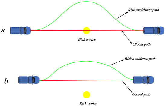
Figure 1.
Schematic diagram of risk avoidance path division. (a) The risk center is on the global path. (b) The risk center is on one side of the global path.
The proposed risk avoidance path planning aims to generate risk avoidance trajectories in the case of risk points in the environment and enable the vehicle to return to the global path. The avoidance trajectory is updated after the vehicle detects the risk point to handle any changes in the risk point location. At the same time, the feasibility of the path planning method is verified by simulation calculation. The entire proposed architecture is shown in Figure 2.
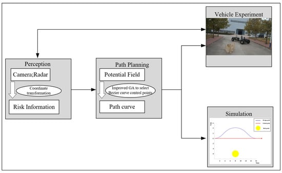
Figure 2.
Overall architecture of risk avoidance system.
As illustrated in Figure 2, the procedure for an autonomous vehicle to evade risk points encompasses the following steps: firstly, the information of risk points must be ascertained, including their location and type. Secondly, an artificial potential field model is constructed based on the risk point information. Utilizing an enhanced genetic algorithm, control points for a Bezier curve path are calculated, resulting in the generation of the path curve. Lastly, this computational process undergoes simulation verification initially on a computer software platform prior to validation in a real-world environment with an actual vehicle.
2.2. Coordinate Transformation Model
In order to facilitate the calculation of the risk avoidance path line, this study converted lon-o-lat (longitude and latitude coordinates) into X-O-Y coordinate system. O is the starting point of a vehicle’s path in the latitude and longitude space. The position of the vehicle at the start of the path line of vehicle risk avoidance (lon0, lat0) is set to the origin of the X-O-Y coordinate system. The driving direction of the global planned path is set to the X-axis direction, and the other vertical direction is set to the Y direction. The coordinate units of latitude and longitude are angles, which need to be converted into radians for calculation. P(lonp, latp) is an arbitrary point in the latitude and longitude space. We can use the following Formula (1) to calculate the coordinate P(xp, yp) of point P(lonp, latp) in the X-O-Y coordinate system:
where R indicates the ellipsoidal radius of the earth, a is major axis of earth, and b is the minor axis of earth. (x′0, y′0) is the position of the vehicle in the X-O-Y coordinate system, which is also the position of the vehicle when the path planning begins. (x′p, y′p) is the position of any point in the lon-o-lat coordinate system and converts latitude and longitude to right-angle coordinates. The θ is the global planned path heading angle of the vehicle, which is the angle between the direction of the X-axis in the X-O-Y coordinate system (the direction of the vehicle) and the direction of lon in the lon-o-lat coordinate system. The coordinate transformation principle is shown in Figure 3.
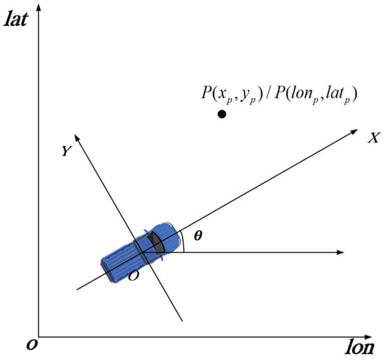
Figure 3.
Coordinate transformation principle.
2.3. Preliminary on Bezier Curve
The type of curve and the parameterization method of the curve have an important influence on path calculation. The Bezier curve was proposed in 1962 by French engineer Pierre Bezier. The Bezier curve is a continuous smooth curve with the characteristics of continuous curvature and simple control, which is very suitable for a geometric description of obstacle avoidance path curves. The set control points are P0, P1… Pn. The n-order Bezier curve of the Pn control can be expressed as
where u indicates the normalized variable. It is crucial to emphasize that in this study, u does not serve as a time parameter for the path curve, nor is it an independent variable that directly shapes the Bezier curve. Instead, the shape of the Bezier curve is governed by control points. In this paper, the coordinates of the control points of the Bezier curve are selected as the independent variables for controlling the shape of the curve. The value of u is used to determine the specific position of a point on the curve. As u varies from 0 to 1, it moves along the path of the curve from the starting point to the ending point. By adjusting the value of u, different points on the curve can be obtained; for example, when u = 0, it represents the initial point of the curve; when u = 0.5, it represents the midpoint of the curve; and when u = 1, it represents the ending point of the curve.
In a two-dimensional X-O-Y plane coordinate system, if the transverse coordinates (x) and longitudinal coordinates (y) of the curve are expressed as functions of the parameter (u), then the nth-order Bezier curve can be expressed as
where (xi, yi), i = 0, 2, 3, 4… n − 1 indicates the coordinate of each control point, x is the abscissa of the Bezier curve, and y is the ordinate of the Bezier curve. The Bezier curve diagram is shown in Figure 4.
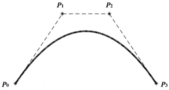
Figure 4.
Bezier curve.
The first and second derivatives of the Bezier curve are expressed as
In the X-O-Y coordinate system, the curvature of a Bezier curve using the curvature formula is calculated. The curvature of the Bezier curve can be expressed as
This is the method for calculating the curvature in Bezier curves. The relationship between path curvature and velocity is discussed in Section 3. In the process of transforming from a global path to a local avoidance path, the curvature of the path should remain continuous. The global path is a straight-line path, and the initial and final points of the obstacle avoidance curve coincide with the global path, so the value of the curvature of these two points should be 0.
The first and second derivatives of the Bezier curve at the initial point are calculated as
The curvature of the Bezier curve at its initial point (u = 0) is calculated as
In the analysis of Formula (10), in order to make the curvature of the initial point of the Bezier curve 0, the following conditions should be met:
According to Formula (11), it can be concluded that the condition that the initial point curvature of the Bezier curve is zero is that the first three control points (P0, P1, P2) are located on the same line. In addition, in the process of switching from the global path to local avoidance path, the derivative of the path curve should be continuous. Therefore, the derivative of the initial point of the Bezier curve is the same as the derivative of the global path. The derivative of the initial point of the Bezier curve is calculated as
From Formula (12), we can conclude that P0 and P1 are on the straight line of the global path. According to the above analysis, in order to satisfy the curvature continuity and derivative continuity of the path, the first three control points (P0, P1, P2) of the Bezier curve are located on the straight line of the global path. By the same analysis, the last three control points (Pn−3, Pn−2, Pn−1) of the Bezier curve are also on the straight line of the global path, as shown in Figure 5.
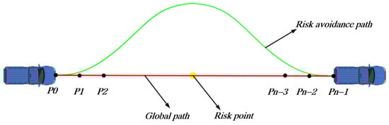
Figure 5.
Risk avoidance path model.
2.4. Path Curve Model for Vehicles
According to the conclusion in Section 2.3, the Bezier curve of the avoidance path has at least six control points located on the straight line of the global path. The number of control points determines the order of the Bezier curve. The higher the order, the more complicated the calculation of the Bezier curve. Under normal circumstances, the distribution of risks in the environment is evenly distributed from the risk point to the surrounding direction. Therefore, the risk avoidance path curve should be symmetrical on both sides of the risk center point. Therefore, in order to reduce the calculation of the path curve, two symmetric Bezier curves are adopted as the path curve of risk avoidance in this paper. The symmetric point of the two Bezier curves has the same horizontal coordinate as the risk center point. And the derivative and curvature of the path curve at the symmetric point should remain continuous. So, the derivatives and curvatures of two Bezier curves are 0 at the point of symmetry. Using a similar calculation procedure as described in Section 2.3, it can be determined that there are at least three control points on each Bezier curve on a line parallel to the X-axis direction. Based on the above analysis, the Bezier curve, as a risk avoidance path, should have at least six control points and be at least a fifth-order Bezier curve.
In this study, a structure splicing two symmetrical fifth-order Bezier curves is used as the path line of vehicle risk avoidance. The control points of the first Bezier curve are P0, P1, P2, P3, P4, and P5, the control points of the second Bezier curve are P5, P6, P7, P8, P9, and P10, and the symmetric line between the two Bezier curves is x = x5. The center of the risk point is also on the line x = x5, as shown in Figure 6. In order to ensure the stability of the vehicle and the smoothness of the path, the curvature of the curve should be kept continuous during the process of switching from the global path line to the risk avoidance path line. The global path advances in the direction of the X-axis, so the curvature of the Bezier curve used in the risk avoidance path line should be 0 at the P0 and P10. At the same time, in order to ensure the continuity of the curvature of the entire risk avoidance path line, the curvature at the junction point (P5) of the two symmetric Bezier curves should be 0, as shown in Figure 6. P1, P2, and P3 are located on the X-axis and have longitudinal coordinates of 0. Similarly, P3, P4, and P5 need to be on a line parallel to the X-axis, with P3 and P4 having the same ordinate as P5.
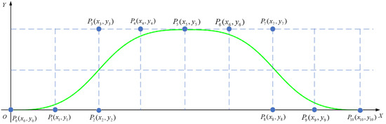
Figure 6.
Control points of the Bezier curve path.
Because the shape of Bezier curve is completely determined by the selected control point coordinates, the problem of ideal risk avoidance path planning based on a fifth-order Bezier curve is transformed into a mathematical optimization problem of seeking coordinates of the control points.
The coordinates of the control points P0(x0, y0), P1(x1, y1), P2(x2, y2), P3(x3, y3), P4(x4, y4), P5(x5, y5), P6(x6, y6), P7(x7, y7), P8(x8, y8), P9(x9, y9), and P10(x10, y10) of the fifth-order Bezier curve have the following relations:
where xrisk is the horizontal coordinate of the risk center point. In order to ensure the continuity of the driving path curve, the following relationship should be satisfied:
According to the above position relationship, different coordinate values are adjusted to obtain different curves, as shown in Figure 7.
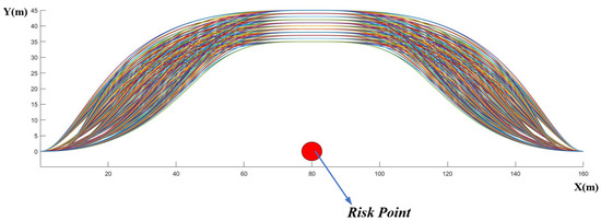
Figure 7.
Bezier curve path cluster.
As shown in Figure 7, multiple curved paths can be generated by adjusting the control points of the Bezier curves. Different paths are distinguished by different colors. However, not all of these curves fulfill the requirements for the desired path curvature variations. Therefore, during the curve optimization process outlined in Section 5, we incorporate these necessary conditions.
3. Vehicle Kinematic Model
To ensure that curved paths align with the driving characteristics of vehicles, this paper employs a vehicle kinematics model, leveraging geometric parameters to analyze the motion of autonomous vehicles. The vehicle dynamics model, being an accurate mathematical representation, enables the derivation of more precise constraints on vehicle operation. The kinematic model for autonomous vehicles is illustrated as referenced in Figure 8 [37,38]. The purpose of this section is to establish the relationship between speed and curvature so that in subsequent simulations and experiments, once the travel speed is set, the maximum limit value of the path curve’s curvature can be calculated.
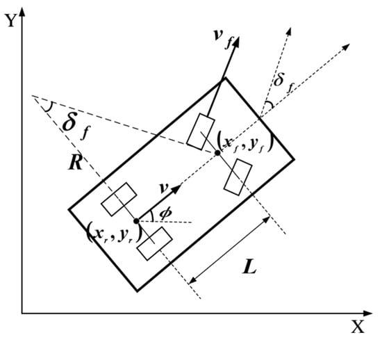
Figure 8.
Vehicle kinematic model.
(xf, yf) are the coordinates of the midpoint of the front axis, (xr, yr) are the coordinates of the midpoint of the rear axis, Ø is the heading angle of the vehicle at a point in time, and L is the wheelbase of the vehicle. vf and vr are the velocities of the midpoint of the front axle and the midpoint of the rear axle, respectively. According to the position relationship between the front and rear axles of the vehicle, the following can be obtained:
, and vr conform to the following relationship:
According to Ackermann’s mathematical geometry relationship, the motion constraints of the front axle and the rear axle of the vehicle are
where δf is the turning angle of the front wheel of the vehicle. By derivation of Formula (15), we can obtain
By calculating Formulas (16)–(18), the angular velocity ω of the vehicle can be obtained as follows:
In the two-degrees-of-freedom model, it is generally believed that the curvature radius of the vehicle trajectory is the same as the instantaneous steering radius when the vehicle begins to turn. The mathematical relationship between the vehicle turning radius and heading angle is as follows:
where R is the turning radius of the vehicle. In the process of driving, the relationship between the front wheel angle of the vehicle δf and the lateral acceleration of the vehicle a_y is
According to the vehicle performance, the maximum lateral acceleration a_ymax can be obtained, and then the minimum turning radius Rmin can be calculated according to the vehicle’s traveling speed. The relationship between the curvature of the path line and the turning radius is
Then, the maximum curvature kmax of the path line can be calculated.
In the process of risk avoidance path planning, the vehicle is assumed to be in a circle, the radius of which is RV, and the center of the danger point cannot appear in the circle. In addition, the maximum angle αmax between the curve and the original path does not exceed 45° [39,40], as shown in Figure 9.
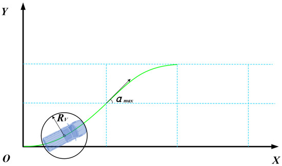
Figure 9.
Vehicle equivalent circle model.
4. Risk Point Model
There are many potential risk points in the environment, such as fire, smoke, land mines, and potential explosions, etc. After determining the location of the danger points, it is necessary to plan and design the obstacle avoidance path to keep a safe distance between the obstacle avoidance path and the risk point so as to avoid the risk point. The closer the vehicle is to the potential risk point, the higher the probability of danger, and the farther the vehicle is from the potential risk point, the lower the probability of danger. This distance-related relationship can be described by the artificial potential field theory.
In the traditional artificial potential field method, there is a repulsive force field and a gravitational field, and the target end point has a gravitational attraction to the vehicle, while the dangerous point repels the vehicle to approach and the vehicle moves under the action of the combined force so it can continue to approach the target. The model constructed in this study is a line of risk avoidance path, which does not need to analyze the influence of the gravitational field of the target points. Therefore, we only consider the repulsive effect of the risk point on the vehicle and generate a static risk point threat potential field to prevent the vehicle from being too close to the risk point.
There are many kinds of potential field functions in artificial potential fields. In this paper, two-dimensional Gaussian distribution is selected as the artificial potential field modeling function, which is suitable for potential risk areas such as explosion risk or land mines. The repulsive force function of the risk point that excludes the vehicle from approaching the risk point can be defined as
where Prisk represents risk value; A is a constant, representing the maximum value of risk. Typically, the value of A is set to one. α is also a constant, representing the attenuation rate; the size of α determines the influence range of the potential field according to the type of risk points in the environment to determine. K represents the distance from the current position to the risk point, where the distance is understood as the distance from the edge of the vehicle to the edge of the risk point not the distance between the center of mass.
For a risk point with known coordinate positions combined with the vehicle circular model in Section 3, the calculation expression of K is as follows:
where (x, y) represents the coordinates of any location on the map and (xrisk, yrisk) is the location of the center of the risk point, RV represents the radius of the vehicle, as shown in Figure 9. The distribution of the repulsion artificial potential field at a risk point is shown in Figure 10.
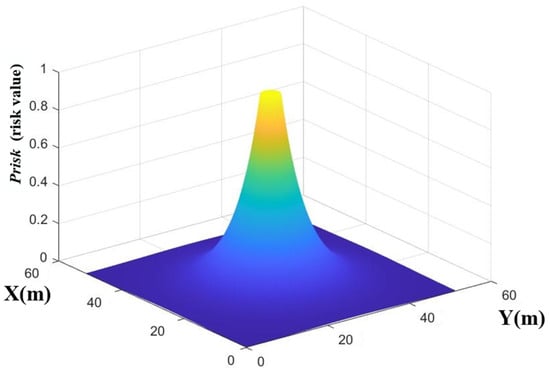
Figure 10.
Artificial potential field distribution model at risk point.
There are many types of risk points in the environment, and the value of α is judged according to the type of risk points. The greater the influence of risk points on the surrounding area, the greater the value of α. The less influence the risk point has on its surroundings, the smaller the value of α, as shown in Figure 11.
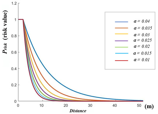
Figure 11.
Risk values with different α.
In order to keep a safe distance between the escape curve path and the risk point, the curve integral of the Bezier curve in the artificial potential field formed by the risk point is calculated, and the result is the sum of the risk value (Ppath) of the entire curve path.
where C is the Bezier curves risk avoidance path in Section 2.3, as shown in Figure 12.
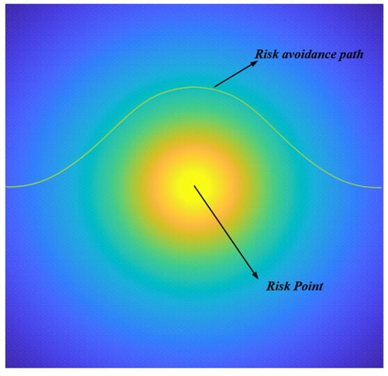
Figure 12.
Bezier curve path in risk point artificial potential field.
5. The Improved Genetic Algorithm
To determine the coordinates of the control points in the Bezier path curve model, this section proposes an improved genetic algorithm.
5.1. Genetic Algorithm
Genetic algorithms (GAs), first introduced by Professor Holland and his research team at Michigan University in 1975, constitute a comprehensive set of theories and methodologies. The GA is grounded in the biological evolution theory proposed by the British naturalist Charles Darwin, drawing inspiration from the natural selection and evolutionary mechanisms of “survival of the fittest” in nature to construct models for artificial systems [41,42,43].
The GA process commences with a population of potential solutions, comprising numerous individuals encoded into specific representations. Each individual, known as a chromosome, is an entity characterized by distinct features. Chromosomes, serving as carriers of genetic material, are collections of multiple genes. The combination of various genes within a chromosome (genotype or internal manifestation) determines the external mutations observed in the individual (phenotype or external manifestation).
The initial step in the GA involves the transformation from phenotype to genotype, a process known as encoding. Following encoding, an initial population is generated. This allows the algorithm to mimic the biological principles of “survival of the fittest” and “natural selection” to evolve solutions through generations. During each generation, individuals are selected based on their fitness values, and genetic operations such as crossover and mutation are employed to produce a new generation of solutions. This iterative process, resembling natural evolution, results in increasingly well-adapted populations that outperform their predecessors. Ultimately, the individuals of the final generation undergo decoding to yield approximate optimal solutions to the problem.
5.2. Improved Genetic Algorithm
In this study, we optimized the selection operator, crossover operator, and mutation operator of the traditional genetic algorithm and simultaneously designed a specialized fitness function to improve the algorithm’s efficiency and solution effectiveness. Below is a detailed introduction to each of these improvements.
5.2.1. Initialize Population
We can consider the avoidance path curve as a symmetric two-segment quintic Bezier curve that represents the phenotype of the path. The expected phenotype of this problem is the Bezier curve path with the lowest risk coefficient in the process of avoiding risk points by unmanned vehicles. Otherwise, we only need the control points to form the Bezier curve. Therefore, the set of control points can represent the chromosome of the path curve. According to the Bezier curve setting in Section 2.4, the starting point (P0) and risk point coordinates of the curve path are determined, and the coordinates of the end point (P10) are also determined according to the symmetry principle. The given starting and ending points are removed from the locus of control from the chromosome. The remaining control points (P1; P2; P3; P4; P5; P6; P7; P8; P9) in the chromosome are made into free control points. The coordinate value of each free control point (x1; y1; x2; y2; x3; y3; x4; y4; x5; y5; x6; y6; x7; y7; x8; y8; x9; y9) acts as a gene in the chromosome. We use the method of generating random numbers to generate the initial population, which can ensure the randomness of the initial population and provide wide diversity for the group.
5.2.2. Fitness Function
The function of fitness function is to calculate the individual values in the population and select the ideal control point coordinates according to the individual fitness values in each generation. In our case, the vehicle path constraints and risk distribution mentioned above are added to the fitness function. According to the vehicle kinematic model analysis in Section 3, the curvature limitation of the path curve can be obtained, so the curvature fitness function is as follows:
According to the limit of the maximum angle between the vehicle driving direction and the horizontal direction in Section 3 the fitness function can be obtained as follows:
According to the limitation that the center of the vehicle and the danger point in Section 3 is less than the radius of the design circle, the fitness function can be obtained as follows:
The fitness function obtained according to Formula (14) is
According to the description in Section 4, the sum of the risk factors of the path line in the artificial potential field is calculated, and the fitness function of the path risk factors is obtained as follows:
Each of the above fitness functions will have an impact on the search process. Therefore, by multiplying these five fitness functions together, we obtain a comprehensive fitness function for the improved genetic algorithm as follows:
This fitness function can satisfy various limitations of the path line and calculate the risk factor of the path. The parameters for minimizing the fitness function are the coordinates of the control points on the curve.
5.2.3. Improved Selection Operator
The purpose of the selection operator is to inherit the optimized individual directly to the next generation or to create a new individual and then to the next generation by pairing. Selection operations are usually based on fitness assessments of individuals in a population, and selection strategies determine whether individuals can be retained and continue to evolve.
Common selection strategies include roulette selection and elite selection. Roulette is a kind of proportional selection; the probability of an individual being selected is proportional to its fitness value. However, because this method is based on probability selection, it often produces large errors, and sometimes individuals with large fitness values cannot be selected. Compared with the roulette method, the elite selection strategy can retain the individuals with the best contemporary fitness value to continue evolution and can also retain the diversity of the population. The disadvantage is that the local optimal individuals are not easy to be eliminated. In view of the advantages and disadvantages of the two methods, this paper adopts the combination of elite selection strategy and roulette method to make individual selection. The specific operation steps are as follows:
- Step 1:
- Population individuals are arranged in ascending order according to non-zero fitness function values.
- Step 2:
- Select the top 25% of individuals from the permutation as the elite selection.
- Step 3:
- Calculate the roulette probability that the remaining entities are selected.
- Step 4:
- Apply roulette to the remaining individuals to select 25% of the total population.
- Step 5:
- Combine the individuals selected in Steps 2 and 4.
Using the above selection method, 50% of the total population can be selected as the elite group. The use of this improved selection operator is to utilize both the roulette wheel selection method to ensure the algorithm’s global search capability and the elitist selection method to ensure the convergence of the algorithm towards the optimal solution.
5.2.4. Improved Crossover Operator
The crossover operator is an important step in genetic algorithms, which simulates the crossover process in biological genetics. The crossover operation creates a new individual by exchanging the chromosomes of two individuals. In this study, the population whose number is 50% of the total population obtained by the selection strategy is calculated by the crossover operator. Each time, two individuals are selected as the mother chromosome and the father chromosome, and the first half of the mother chromosome is combined with the second half of the father chromosome to produce the chromosome of the first child. Combining the second half of the mother’s chromosome with the first half of the father’s chromosome produces the second child’s chromosome, so that each parent produces two children, and 50% of the number of populations produces a new population with the same total number of populations through the crossover operator.
The use of the crossover operator is to generate new individuals within the global scope, thereby enhancing the algorithm’s global search capability. By employing the crossover operator, the algorithm is able to explore new regions within the solution space, thereby increasing the diversity of the population.
5.2.5. Improved Mutation Operator
Mutation is to randomly change the value of some genes in an individual, which simulates the process of mutation in biological heredity. The mutation operation is to increase the diversity of the population. In this work, mutations are formed by a crossover process and then randomly reproduce a certain number of offspring. Because the mutation range of traditional random mutation operators is large, it is not conducive to the local optimization of the algorithm. According to the characteristics of the problem in this study, two mutation operators, global mutation, and local mutation, were proposed to adapt to each evolutionary stage of the population.
Global mutation (global search) is the random modification of a gene and then the random generation of a gene set for the selected offspring. This type of mutation helps genetic algorithms explore large areas, increasing the diversity of the population and helping to find viable solutions. However, the mutation range of the global mutation operator is large, which is not conducive to the local optimization of the algorithm.
Local mutation (local search): Local mutation is achieved by the random modification of each gene on the chromosome of the selected progeny in its local environment. The local environment is a bounded range defined by the gene centered at the selected point and the given radius as the local search range radius. This type of mutation facilitates local optimization, using the neighbors of the dominant individual to find the best new path, reducing the amount of test data computation.
The path with the highest fitness value in each generation is called the dominant individual. This optimal individual is preserved in the next generation, regardless of the mutation operator. If the optimal individual of successive generations is always changing, the fitness value of the optimal individual is also greatly reduced, and the optimal individual cannot remain unchanged for multiple generations, indicating that the diversity of the population is required at this time, so more global mutation is needed.
The optimal individual for many successive generations is not affected by the mutation until it is replaced by other dominant individuals with higher fitness values. When the diversity of a population is not best improved over many successive generations, it means that global mutations become computationally inefficient. In this case, more local mutation should be used to find the optimal solution and improve the efficiency of calculation.
The mutation operator of this paper is the combination of global mutation and local mutation. Firstly, the local search range radius of local mutation is set. When the historical optimal individual does not change for more than 20 generations and the fitness function value of the optimal individual decreases over 40% compared with that of the original individual, the probability of a local mutation is 60%. Otherwise, the probability of a global mutation is 60%.
The use of this improved mutation operator is to emphasize global search during the initial stages of the search process, enabling the algorithm to quickly locate the range of optimal solutions and then shift its focus to local search during the later stages, which facilitates the algorithm to find local optimal solutions more rapidly.
The flowchart of the improved genetic algorithm is shown in Figure 13.
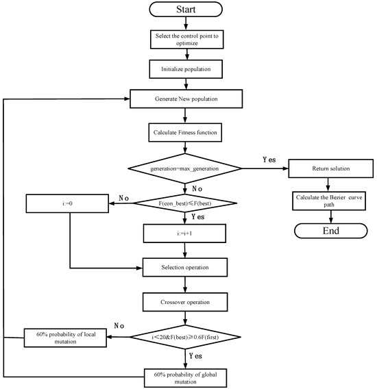
Figure 13.
Improved flowchart of genetic algorithm.
6. Simulation Results and Analysis
In this section, a new strategy combining a Bezier curve and the improved genetic algorithm is adopted to deal with the risk point avoidance path planning problem of the unmanned vehicle in Figure 1. The improved genetic algorithm is used to optimize the control point coordinates of the Bezier curve, and then the path of the Bezier curve is obtained. To verify the effectiveness of the algorithm, Windows 11 was used as the platform and Matlab2022 was used to simulate the programming condition. The emulation hardware platform is an Intel Core (TM) i7-8700 CPU@GHz processor with a clock speed of 3.20 GHz and 16 GB of RAM. Other parameters are described as follows:
- Vehicle parameters: If the wheelbase length L of the vehicle is 3 m, the maximum lateral acceleration of the vehicle (a_y) is 0.4 g, and the maximum driving speed of the vehicle during the risk avoidance period is 4 m/s, the maximum curvature (kmax) of the vehicle’s driving path line can be obtained as 0.31. In addition, the radius (RV) of the vehicle equivalent circle is set to 2.7 m.
- Genetic algorithm parameters: the population size was set to 100 and the local search range radius was set to 0.2 m.
In order to more intuitively represent the logic of the algorithm, the position parameters and geometric size parameters in this part of the simulation are set in the X-O-Y coordinate system, with the unit of length being meters (m).
6.1. Scenario 1
The direction of the global path is the positive direction of the X-axis. The risk point is set on the global path. The coordinates of the starting point of the risk avoidance path are set to (0, 0) and the coordinates of the risk point are set to as (10, 0). The maximum risk value A of the risk point is one, and the influence factor α of the risk point is 0.02. The simulation results show that the coordinates of the control points are P0(0, 0), P1(0.967, 0), P2(4.281, 0), P3(4.055, 5.227), P4(8.420, 5.227), P5(5, 5.227), P6(11.580, 5.227), P7(15.945, 5.227), P8(15.719, 0), P9(19.033, 0), and P10(20, 0), and the fitness function value of the optimal solution is 20.4684. The fitness function value of the genetic algorithm is shown in Figure 14.
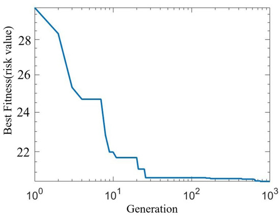
Figure 14.
Result diagram of population fitness value in scenario 1.
The literature [32] proposes an obstacle avoidance path planning algorithm that combines the genetic algorithm with cubic Bezier curves. We have chosen this algorithm to compare the performance with the algorithm presented in this paper. The result of the path planning is shown in Figure 15, which depicts three paths. The yellow circle represents the risk points, the global path is a red line, the path curve (path1) calculated by the algorithm in this paper is a blue line, and the path curve (path2) calculated by the algorithm in the literature [32] is a green line.
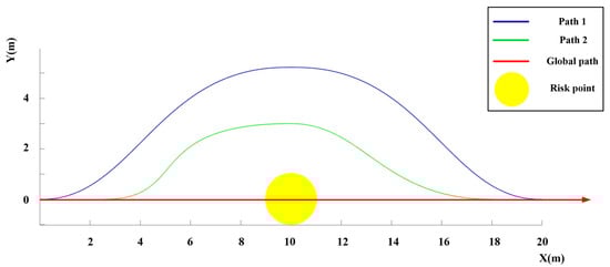
Figure 15.
Path planning results of different algorithms.
The curvature of the Bezier curve path is shown in Figure 16a, and the angle between it and the global path is shown in Figure 16b. Additionally, the curvature of path1 and path2 is shown in Figure 16a, while the angle between the path curve and the global path of path1 and path2 is shown in Figure 16b.
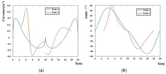
Figure 16.
(a) The curvature of the paths; (b) the angle of the paths.
By analyzing the simulation results of Figure 15 and Figure 16 and comparing the path (path2) obtained by the algorithm in reference [32] with the path (path1) derived from the algorithm in this paper, it is found that the length of path1 has increased by 6.3 m, while the path risk coefficient has decreased by 15%. Additionally, the maximum angle between the path curve and the global path has diminished by 4.9 degrees, and the maximum curvature of the path curve has reduced by 0.16. The travel time of the path (path1) obtained by the algorithm in this paper is 5.83 s, which is in line with the vehicle driving characteristics.
The simulation results from scenario 1 indicate that the fitness function in Figure 14 exhibits significant variations during the initial stage of the search process, with reduced variations in the later stages. This is attributed to the modification of the genetic algorithm’s operators, which directs the search towards a global exploration in the early phase and shifts towards a local search in the later phase. The path curve depicted in Figure 15 is a curved trajectory that intentionally keeps a safe distance from risk points, and this path is also characterized by its smoothness. In Figure 16, the curvature and angles of the path curve align with the dynamic characteristics of vehicles, which is a result of incorporating curvature and angle constraints into the fitness function of the genetic algorithm.
6.2. Scenario 2
The direction of the global path is also the positive direction of the X-axis. The risk point is set on the side of the global path. The coordinates of the starting point of the risk avoidance path are set to (0, 0) and the coordinates of the risk point are set to (8, −6). The maximum risk value A of the risk point is one, and the influence factor α of the risk point is 0.02.
The simulation results show that the coordinates of the control points are P0(0, 0), P1(0.5968, 0), P2(4.280, 0), P3(2.5176, 4.1640), P4(7.5544, 4.1640), P5(5, 4.1640), P6(8.4456, 4.1640), P7(13.4824, 4.1640), P8(11.72, 0), P9(15.4032, 0), and P10(16, 0), and the fitness function value of the optimal solution is 14.0443. The fitness function value of the genetic algorithm is shown in Figure 17.
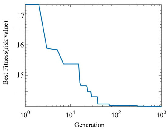
Figure 17.
Result diagram of population fitness value in Scenario 2.
The Bezier curve path results have been illustrated in Figure 18. In Figure 18, the yellow circle represents the risk points, the global path is a solid red line, and the designed risk avoidance path curve is a solid blue line.
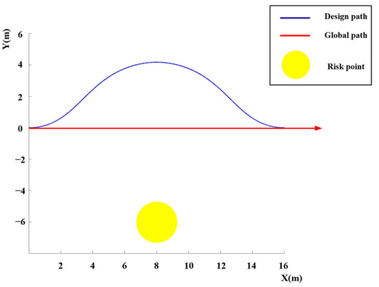
Figure 18.
The Bezier curve path in Scenario 2.
The curvature of the Bezier curve path is shown in Figure 19a, and the angle between it and the global path is shown in Figure 19b.
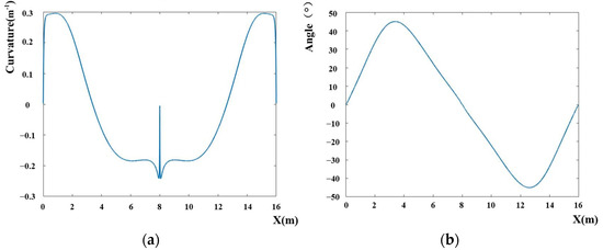
Figure 19.
(a) The curvature of the Bezier curve path; (b) the angle of the Bezier curve path.
Scenario 2 has also resulted in a smooth curved path that keeps a safe distance from risk points; the path length is 18.60 m and the travel time is 4.65 s.
Two examples Section 6.1 and Section 6.2 prove that the improved genetic algorithm can optimize the control points of the Bezier curve according to the kinematic constraints of the vehicle and the distribution of risk points in the environment. Then, the risk avoidance path curve can be calculated using the control points obtained. Two simulation results show that the proposed method can provide a feasible path for unmanned vehicles to avoid risk points. The curvature of the designed curved path is continuous, and the path is smooth, which can meet the driving conditions of the vehicle. The most important thing is that the curved path of this design can sufficiently remove the vehicle from the risk point. Furthermore, we have set up various vehicle types and different maps, and the simulation results have consistently yielded appropriate curved paths to avoid risk points, indicating that the algorithm presented in this paper exhibits excellent adaptability and robustness.
The operation time of scenario 1 is 2.167 s and that of scenario 2 is 2.496 s. The operation time includes both the optimization computation of the improved GA algorithm and the computation of the Bezier curve. After further optimization of the computing environment and vehicle configuration in the future, the calculation time can also be shortened to meet the real-time computing needs of autonomous vehicles.
In the two scenarios above, the improved genetic algorithm proposed in this paper is compared with several other optimization algorithms, including particle swarm optimization (PSO), simulated annealing (SA), and ant colony optimization (ACO). The comparison results are shown in Figure 20. It can be observed that the path results obtained using the improved genetic algorithm have the lowest risk value. Compared to PSO, it reduces the risk factor by approximately 25%; compared to SA, it reduces it by approximately 15%; and compared to ACO, it reduces it by approximately 20%.
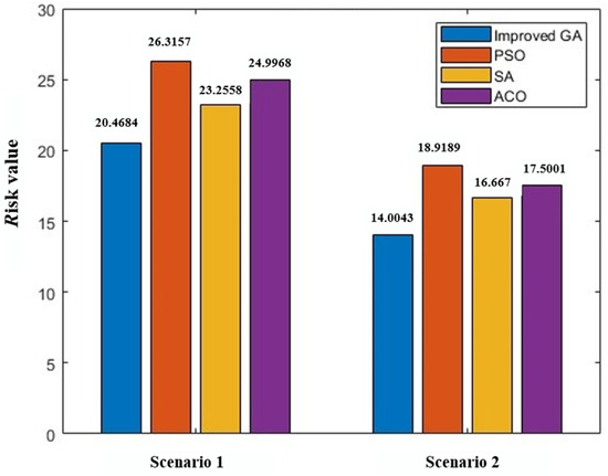
Figure 20.
Optimization results of different algorithms.
7. Actual Condition Verification
In this paper, a modified electric drive test vehicle with an automatic navigation function is used as the experimental platform, as shown in Figure 21. This test vehicle has remote control and positioning and navigation functions. It is equipped with an automatic steering system, remote control system, millimeter wave radar, visual measurement system, remote information transmission system, monitoring system, and other information and control systems. The specific parameters of the test vehicle are shown in Table 1. The experiment was conducted at a vehicle test site in Xianyang, Shaanxi Province, where there are closed internal roads where we can set up artificial risk points.
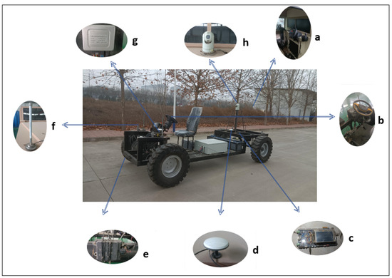
Figure 21.
(a) Navigation control terminal; (b) steering actuator; (c) positioning system processor; (d) Beidou positioning antenna; (e) vehicle-mounted millimeter wave radar; (f) data transmission antenna; (g) vehicle steering controller; (h) video capture device.

Table 1.
The parameters of the test vehicle.
On the experimental platform, an industrial computer running the Windows 10 operating system was installed. The software for the entire experimental system was developed using the MATLAB2022 programming language, while the hardware was controlled by a microcontroller. Data transmission between the software and hardware was facilitated through the CAN bus. The experiment was conducted in a closed facility in Xianyang, Shaanxi Province, where the internal roads were isolated from external influences, allowing us to set up simulated risk points along these roads. The unmanned vehicle was initially set to move in a straight direction towards the north. A risk point was placed on the vehicle’s original path. The starting coordinates of the curved path designed to avoid the risk point and the coordinates of the risk point itself are detailed in Table 2.
Table 2.
The coordinates of the starting point and the risk point.
During the avoidance period, the maximum speed of the vehicle is 4 m/s, and the maximum curvature of the vehicle path line (kmax) can be calculated as 0.34. The population of the improved genetic algorithm is set to 100, and the local search range radius is set to 0.1 m. Then, the parameters for the risk point are set; the maximum risk value A of the risk point is one and the influence factor α of the risk point is 0.03.
In Figure 22a, the vehicle is still on the global path, and the sensor device on the vehicle detects that there is a risk point on the current path and starts the risk avoidance operation. The process of risk avoidance operation is shown in Figure 22b–e. When the vehicle bypasses the risk point, the end of the Bezier curve returns the vehicle to the global path, as shown in Figure 22f.
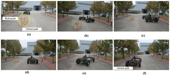
Figure 22.
Experimental platform and experimental site. (a) The vehicle was driving along the global path, identified the risk point and began path planning; (b–e) The vehicle was driving along the planned Bezier curve path; (f) The vehicle bypassed the risk point, it continued to follow the global path.
The computation results show that the coordinates of the control points are shown in Table 3, and the fitness function value of the optimal solution is 16.926. The fitness function value of genetic algorithm is shown in Figure 23.
Table 3.
The coordinates of the control points of the path curve.
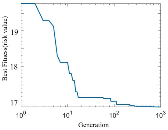
Figure 23.
Result diagram of population fitness value in experiment.
The results of the risk point avoidance path are shown in Figure 24.
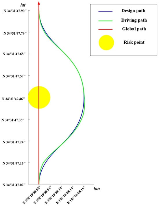
Figure 24.
The path curve for avoiding risks on the experimental platform.
As can be seen from Figure 24, the risk point avoidance path planned by the algorithm in this paper is a smooth curved path and can meet the driving conditions of vehicles. In summary, this paper provides a reliable path planning method for avoiding the risk points of unmanned vehicles.
8. Conclusions
The automatic identification of risk points and automatic avoidance of risk points are of great significance to the safe and efficient execution of tasks by unmanned vehicles. In this paper, a new path planning strategy for unmanned vehicles avoiding risk points is proposed, which combines a Bezier curve with an improved genetic algorithm. This new strategy includes several innovations. First, two symmetrical fifth-order Bessel curves are designed as the curves of the path. The strategy in this paper can keep the curvature of the path continuous when the vehicle is connecting between the global path and the risk avoidance path. Secondly, the artificial potential field model is used to describe the risk points. This is because the influence range of the risk point changes with the distance, and the risk value of the path can be expressed by calculating the integral of the path curve in the artificial potential field formed by the risk point. Thirdly, an improved genetic algorithm is proposed to optimize the control points of the Bezier curve. The maximum curvature limit, the maximum heading angle limit, and the risk value of the path are added to the fitness function of the genetic algorithm. At the same time, the selection operator and mutation operator of the algorithm are improved. A new selection operator is obtained by combining the elite selection strategy with a roulette. Mutation operators are divided into global mutation and local mutation. The improved genetic algorithm can find the optimal solution more efficiently.
The simulation results show that this method can calculate a risk point avoidance curve path with less risk under the premise of curvature limitation and angle limitation. Then, we carried out the actual working condition verification. The results show that the new strategy in this paper can provide an effective path planning scheme for unmanned vehicles to avoid risk points. The algorithm designed in this paper exhibits excellent computational accuracy. However, its application environment is confined to standard structured settings, and complex environmental factors have not been taken into consideration. Therefore, further enhancements are required to improve the robustness of the algorithm.
Regarding future work, our next research priorities encompass (1) further refining the computational strategy of the genetic algorithm to make the enhanced version more adept at optimizing the control points of Bezier curves and (2) applying the algorithm proposed in this paper to more complex environments.
Author Contributions
Conceptualization, L.F. and G.X.; methodology, L.F. and G.X.; software, G.X. and Y.L.; formal analysis, D.G. and Z.Q.; investigation, L.F. and G.X.; resources, X.S. and G.X.; writing—original draft preparation, G.X. and X.S.; writing—review and editing, G.X. and J.C.; project administration, L.F., G.X., and X.S. All authors have read and agreed to the published version of the manuscript.
Funding
This research received no external funding.
Data Availability Statement
The raw data supporting the conclusions of this article will be made available by the authors upon reasonable request.
Acknowledgments
The authors declare that they have no known competing financial interests or personal relationships that could have appeared to influence the work reported in this paper.
Conflicts of Interest
The authors declare no conflicts of interest.
References
- Wang, R.; Wan, J.; Ye, Q.; Ding, R. Path Tracking and Anti-Roll Control of Unmanned Mining Trucks on Mine Site Roads. World Electr. Veh. J. 2024, 15, 167. [Google Scholar] [CrossRef]
- Karma, S.; Zorba, E.; Pallis, G.C.; Statheropoulos, G.; Balta, I.; Mikedi, K.; Vamvakari, J.; Pappa, A.; Chalaris, M.; Xanthopoulos, G.; et al. Use of unmanned vehicles in search and rescue operations in forest fires: Advantages and limitations observed in a field trial. Int. J. Disaster Risk Reduct. 2015, 13, 307–312. [Google Scholar] [CrossRef]
- Zhao, X.; Lv, Z.; Qiu, Q.; Wu, Y. Designing two-level rescue depot location and dynamic rescue policies for unmanned vehicles. Reliab. Eng. Syst. Saf. 2023, 233, 109119. [Google Scholar] [CrossRef]
- Zhang, H.; Yang, X.; Liang, J.; Xu, X.; Sun, X. Gps path tracking control of military unmanned vehicle based on preview variable universe fuzzy sliding mode control. Machines 2021, 9, 304. [Google Scholar] [CrossRef]
- Wang, N.; Li, X.; Zhang, K. A survey on path planning for autonomous ground vehicles in unstructured environments. Machines 2024, 12, 31. [Google Scholar] [CrossRef]
- Dawid, W.; Pokonieczny, K. Methodology of using terrain possibility maps for planning the movement of troops and navigation of unmanned ground vehicles. Sensors 2021, 21, 4682. [Google Scholar] [CrossRef] [PubMed]
- Xu, L.; Cao, M.; Song, B. A new approach to smooth path planning of mobile robot based on quartic Bezier transition curve and improved PSO algorithm. Neurocomputing 2022, 473, 98–106. [Google Scholar] [CrossRef]
- Xie, L.; Xue, S.; Zhang, J. A path planning approach based on multi-direction A* algorithm for ships navigating within wind farm waters. Ocean. Eng. 2019, 184, 311–322. [Google Scholar] [CrossRef]
- Melchior, P.; Orsoni, B.; Lavialle, O.; Poty, A.; Oustaloup, A. Consideration of obstacle danger level in path planning using A* and fast-marching optimisation: Comparative study. Signal Process. 2003, 83, 2387–2396. [Google Scholar] [CrossRef]
- Ji, J.; Khajepour, A.; Melek, W.W.; Huang, Y. Path planning and tracking for vehicle collision avoidance based on model predictive control with multiconstraints. IEEE Trans. Veh. Technol. 2016, 66, 952–964. [Google Scholar] [CrossRef]
- Gasparetto, A.; Boscariol, P.; Lanzutti, A.; Vidoni, R. Path planning and trajectory planning algorithms: A general overview. Motion Oper. Plan. Robot. Syst. Backgr. Pract. Approaches 2015, 01, 3–27. [Google Scholar]
- Fang, Y.; Hu, J.; Liu, W.; Shao, Q.; Qi, J.; Peng, Y. Smooth and time-optimal S-curve trajectory planning for automated robots and machines. Mech. Mach. Theory 2019, 137, 127–153. [Google Scholar] [CrossRef]
- Wang, H.; Wang, H.; Huang, J.; Zhao, B.; Quan, L. Smooth point-to-point trajectory planning for industrial robots with kinematical constraints based on high-order polynomial curve. Mech. Mach. Theory 2019, 139, 284–293. [Google Scholar] [CrossRef]
- Li, W.; Wang, J.; Duan, J. Lane changing trajectory planning of intelligent vehicles based on polynomials. Comput. Eng. Appl. 2012, 48, 242–245. [Google Scholar]
- Berglund, T.; Brodnik, A.; Jonsson, H.; Staffanson, M.; Soderkvist, I. Planning smooth and obstacle-avoiding B-spline paths for autonomous mining vehicles. IEEE Trans. Autom. Sci. Eng. 2009, 7, 167–172. [Google Scholar] [CrossRef]
- Qu, P.; Li, L.; Ren, X.; Jing, L. B-spline Curve based Trajectory Planning for Autonomous Vehicles. Comput. Knowl. Technol. 2016, 26, 235–237. [Google Scholar]
- Brezak, M.; Petrović, I. Real-time approximation of clothoids with bounded error for path planning applications. IEEE Trans. Robot. 2013, 30, 507–515. [Google Scholar] [CrossRef]
- Piccinini, M.; Gottschalk, S.; Gerdts, M.; Biral, F. Computationally efficient minimum-time motion primitives for vehicle trajectory planning. IEEE Open J. Intell. Transp. Syst. 2024, 5, 642–655. [Google Scholar] [CrossRef]
- Zhang, C.; Zhang, X.; Yang, W.; Zhang, G.; Wan, J.; Lei, M.; Dong, D. Safe Path Planning Method Based on Collision Prediction for Robotic Roadheader in Narrow Tunnels. Mathematics 2025, 13, 522. [Google Scholar]
- Han, L.; Yashiro, H.; Nejad, H.T.N.; Do, Q.H.; Mita, S. Bezier curve based path planning for autonomous vehicle in urban environment. In Proceedings of the 2010 IEEE Intelligent Vehicles Symposium, La Jolla, CA, USA, 21–24 June 2010; pp. 1036–1042. [Google Scholar]
- Du, L.; Fan, Y.; Gui, M.; Zhao, D. A Multi-Regional Path-Planning Method for Rescue UAVs with Priority Constraints. Drones 2023, 7, 692. [Google Scholar] [CrossRef]
- Machmudah, A.; Shanmugavel, M.; Parman, S.; Manan, T.S.A.; Dutykh, D.; Beddu, S.; Rajabi, A. Flight trajectories optimization of fixed-wing UAV by bank-turn mechanism. Drones 2022, 6, 69. [Google Scholar] [CrossRef]
- Duraklı, Z.; Nabiyev, V. A new approach based on Bezier curves to solve path planning problems for mobile robots. J. Comput. Sci. 2022, 58, 101540. [Google Scholar] [CrossRef]
- Türkkol, B.Z.; Altuntaş, N.; Çekirdek Yavuz, S. A Smooth Global Path Planning Method for Unmanned Surface Vehicles Using a Novel Combination of Rapidly Exploring Random Tree and Bézier Curves. Sensors 2024, 24, 8145. [Google Scholar] [CrossRef] [PubMed]
- Ahn, S.; Oh, T.; Yoo, J. Collision Avoidance Path Planning for Automated Vehicles Using Prediction Information and Artificial Potential Field. Sensors 2024, 24, 7292. [Google Scholar] [CrossRef] [PubMed]
- Hassani, V.; Lande, S.V. Path planning for marine vehicles using Bézier curves. IFAC-Pap. 2018, 51, 305–310. [Google Scholar] [CrossRef]
- Ma, L.; Yang, J.; Zhang, M. A Two-Level Path Planning Method for On-Road Autonomous Driving. In Proceedings of the Second International Conference on Intelligent System Design and Engineering Application, Sanya, China, 6–7 January 2012; pp. 661–664. [Google Scholar]
- Choi, J.W.; Curry, R.; Elkaim, G. Piecewise bezier curves path planning with continuous curvature constraint for autonomous driving. Mach. Learn. Syst. Eng. 2010, 01, 31–45. [Google Scholar]
- Bae, I.; Moon, J.; Park, H.; Kim, J.H.; Kim, S. Path Generation and Tracking Based on a Bézier Curve for a Steering Rate Controller of Autonomous Vehicles. In Proceedings of the International IEEE Conference on Intelligent Transportation Systems, The Hague, The Netherlands, 6–9 October 2013; pp. 436–441. [Google Scholar]
- Tharwat, A.; Elhoseny, M.; Hassanien, A.E.; Gabel, T.; Kumar, A. Intelligent Bézier curve-based path planning model using Chaotic Particle Swarm Optimization algorithm. Clust. Comput. 2019, 22, 4745–4766. [Google Scholar] [CrossRef]
- Elhoseny, M.; Tharwat, A.; Hassanien, A.E. Bezier curve based path planning in a dynamic field using modified genetic algorithm. J. Comput. Sci. 2018, 25, 339–350. [Google Scholar] [CrossRef]
- Song, B.; Wang, Z.; Zou, L. An improved PSO algorithm for smooth path planning of mobile robots using continuous high-degree Bezier curve. Appl. Soft Comput. 2021, 100, 106960. [Google Scholar] [CrossRef]
- Song, B.; Wang, Z.; Sheng, L. A new genetic algorithm approach to smooth path planning for mobile robots. Assem. Autom. 2016, 36, 138–145. [Google Scholar] [CrossRef]
- Chen, H.; Xie, H.; Sun, L.; Shang, T. Research on Tractor Optimal Obstacle Avoidance Path Planning for Improving Navigation Accuracy and Avoiding Land Waste. Agriculture 2023, 13, 934. [Google Scholar] [CrossRef]
- Li, H.; Luo, Y.; Wu, J. Collision-free path planning for intelligent vehicles based on Bézier curve. IEEE Access 2019, 7, 123334–123340. [Google Scholar] [CrossRef]
- Luan, P.G.; Thinh, N.T. Hybrid genetic algorithm based smooth global-path planning for a mobile robot. Mech. Based Des. Struct. Mach. 2023, 51, 1758–1774. [Google Scholar] [CrossRef]
- Chen, J.; Xu, Y.; Zheng, Z. Neural Network and Extended State Observer-Based Model Predictive Control for Smooth Braking at Preset Points in Autonomous Vehicles. Drones 2024, 8, 273. [Google Scholar] [CrossRef]
- Feng, J.; Yang, Y.; Zhang, H.; Sun, S.; Xu, B. Path Planning and Trajectory Tracking for Autonomous Obstacle Avoidance in Automated Guided Vehicles at Automated Terminals. Axioms 2023, 13, 27. [Google Scholar] [CrossRef]
- Korzeniowski, D.; Ślaski, G. Method of planning a reference trajectory of a single lane change manoeuver with Bezier curve[C]//IOP Conference Series: Materials Science and Engineering. IOP Publ. 2016, 148, 012012. [Google Scholar]
- Ren, D.; Zhang, G.; Wu, H. Reference Modelof Desired Yaw Anglefor Automated Lane Changing Behavior of Vehicle. J. Harbin Inst. Technol 2016, 23, 23–33. [Google Scholar]
- Yu, X.; Gao, X.; Wang, L.; Wang, X.; Ding, Y.; Lu, C.; Zhang, S. Cooperative multi-UAV task assignment in cross-regional joint operations considering ammunition inventory. Drones 2022, 6, 77. [Google Scholar] [CrossRef]
- Tang, J.; Liu, D.; Wang, Q.; Li, J.; Sun, J. Probabilistic Chain-Enhanced Parallel Genetic Algorithm for UAV Reconnaissance Task Assignment. Drones 2024, 8, 213. [Google Scholar] [CrossRef]
- Chen, G.; Zhao, C.; Gong, H.; Zhang, S.; Wang, X. Formation Transformation Based on Improved Genetic Algorithm and Distributed Model Predictive Control. Drones 2023, 7, 527. [Google Scholar] [CrossRef]
Disclaimer/Publisher’s Note: The statements, opinions and data contained in all publications are solely those of the individual author(s) and contributor(s) and not of MDPI and/or the editor(s). MDPI and/or the editor(s) disclaim responsibility for any injury to people or property resulting from any ideas, methods, instructions or products referred to in the content. |
© 2025 by the authors. Licensee MDPI, Basel, Switzerland. This article is an open access article distributed under the terms and conditions of the Creative Commons Attribution (CC BY) license (https://creativecommons.org/licenses/by/4.0/).