1. Introduction
In the last few years, owing to advancements in sensor technology and wireless communication technology, technologies related to UAVs have grown progressively mature and widely applied in various fields [
1]. Compared to manned aircraft, UAVs avoid constraints such as pilot casualties and the need for pilot training, allowing more efficient task execution. Benefiting from advantages such as small size, low cost, and high maneuverability, UAVs demonstrate great potential in both military and civilian domains [
2].
However, as task requirements become increasingly complex, the limitations of single UAV in anti-interference capability and perception range have become more pronounced. The focus of research has shifted toward the collaboration of multi-UAV to execute tasks.
In the field of multi-UAV collaboration, target searching is fundamental and critical. It requires that the UAV swarm be able to efficiently find specific targets in unknown and complex environments. Most existing UAV systems rely on pre-programmed algorithms or real-time control by ground operators, and these methods often exhibit clear limitations in dealing with dynamic environment changes and complex tasks [
3]. Faced with unknown terrains or emergency situations, the adaptability of preset programs is insufficient, while manual remote control is constrained by communication delays and the operator experience.
In this context, the dynamic path planning technology for searching becomes particularly important. It enables UAVs to adapt in real time to changes in their environment and optimize their choices, ensuring they can flexibly complete tasks in complex search environments. To improve the efficiency of target searches, Deep Reinforcement Learning (DRL) demonstrates unique advantages as a machine learning method. DRL allows agents to learn an optimal strategy through interaction with the environment, enabling machines to possess autonomous decision-making capabilities through continuous iteration. Thus, enabling multi-UAV to independently process environment information and make appropriate decisions during task execution through DRL has become a major challenge in the current research field.
During the application process, several difficulties have emerged. On one hand, DRL requires extensive exploration and trial-and-error processes, which can be prohibitively costly in real-world environments. Based on this situation, many studies build simulation environments in a lightweight way. However, these simulation environments often involve multiple agents and targets, resulting in complex state space and action space that complicate modeling and resolution [
4]. On the other hand, the input of DRL algorithm should be the state information of the environment. But UAVs cannot directly observe the comprehensive search environment, which leads to biased evaluations of the action. Therefore, improving DRL algorithms for partially observable problems is an essential consideration for researchers [
5].
To this end, this paper proposes a multi-UAV collaborative work framework, which utilizes physical force field, value reinforcement learning, and multi-agent theory to achieve multi-UAV collaborative target search in partially observable environments. The main contributions are listed as follows.
The Markov Decision Process (MDP) model of the UAV target search problem is established with the proper action space, state space, and reward function that contains various conditions. This model lays the foundation for algorithm design and simulation experiment construction, providing a framework and direction for modeling similar problems in the future.
A novel value-based deep reinforcement learning model, Patricianly Observable Deep Q-Network (PODQN), is proposed based on the Deep Q-Network (DQN) algorithm. The PODQN algorithm can maintains historical observations to understand the whole environment in partially observable scenarios without relying on global state information. Furthermore, it achieves more accurate evaluations of each action through optimizations such as target network and dueling architecture.
The PODQN model is extended to a multi-agent framework for partially observable problems, allowing each agent to use its own experience to train a general network, thus accelerating model convergence.
This paper is organized as follows.
Section 2 reviews the related research on UAV target search.
Section 3 discusses the MDP model established for the problem.
Section 4 presents the proposed PODQN model.
Section 5 describes the simulation experiments and compares the model with other algorithms.
Section 6 shows the conclusions and future work.
2. Related Work
In the field of target search, conventional solutions rely on geometric search algorithms to find all targets by maximizing the coverage of the assigned area [
6]. In multi-UAV search tasks, breadth-first search is widely used. UAVs progressively explore along the boundary according to the detection range of the sensor in the designated search area [
7]. In addition, spiral searches let UAVs move in a circular path around a center and gradually reduce the circle’s radius, which achieves a comprehensive search of the assigned task area [
8,
9]. However, as an exhaustive strategy, the application of geometric search algorithms is limited in practice. This is particularly the case when facing dynamic targets, where the lack of robustness in these algorithms is significant. The movement of dynamic targets may result in ineffective tracking, especially from unexplored to explored areas [
10,
11,
12,
13]. In sparse search environments with few targets, exhaustive searches lead to unnecessary time and resource consumption. Solutions to this problem include partitioning the task area into multiple sub-areas and effectively distributing UAVs using task allocation algorithms.
Currently, the grid partitioning and Voronoi diagram-based partitioning are two prevalent methods for partitioning areas. Vinh et al. used the uniform grid partitioning to address issues in convex polygonal areas [
14]. They divided the area into several equal-area rectangles based on the UAVs’ flight time and speed, achieving collaborative search by assigning different sections to various UAVs. Xing et al. recursively divided the area into multiple sub-polygons using sweep lines [
15]. These sweep lines are used to perform equal-area cuts to preserve the right angles of the original area, which can improve the efficiency of search coverage. Chen et al. employed the weighted balanced graph to partition the entire environment into responsibility areas for each UAV [
16]. By updating the labels of each region based on neighboring regions, it can select a connected area for each UAVs through a defined function. However, in non-uniformly distributed scenarios, the grid partitioning may waste a lot of computational resources in data-sparse areas [
17]. In contrast, the Voronoi diagram partitioning can automatically adjust according to the distribution of point sets. Huang et al. mapped unknown domains into Voronoi diagrams for collaborative search based on the measurement matrix and measurement noise, not only preventing collisions between UAVs but also reducing the computational complexity to linear [
18].
In the search methods described above, the task region is partitioned into several sub-regions and assigned to each UAV [
19]. While this approach is relatively simple, it lacks collaboration among UAVs [
20]. Heuristic algorithms, particularly those that simulate the intelligent behaviors of biological swarms in nature, offer an idea to address this issue. The inspiration for these algorithms comes from the collective behaviors of biological entities in nature, such as flocks of birds and colonies of ants, showcasing impressive collaboration and self-organization [
21]. It is able to efficiently accomplish complex tasks without centralized control, similarly to collaborative searches by UAV swarms [
22]. Kashino et al. set the target appearance probability and search environment confidence as optimization objectives, employing genetic algorithms to make the optimal search [
23]. Zhang and Chen transformed the collaborative search problem into a multi-factor optimization problem, including reconnaissance gains, flight consumption, and flight time [
24]. They improved the Harmony Search Algorithm for multi-UAV collaborative reconnaissance result in faster convergence and greater benefits. Considering that genetic algorithms are susceptible to local optima, Yang et al. integrated repulsive forces simulated by artificial potential fields into the heuristic function of ant colony algorithms [
25]. Moreover, they introduced an adaptive pheromone evaporation factor to dynamically update the pheromone volatility coefficient, gradually diminishing it to the minimum. Compared to traditional ant colony algorithms, the improved algorithm can generate shorter trajectory lengths.
Collaborative target searching based on heuristic algorithms abstracts the search process as an optimization problem and seeks its optimal solution to achieve target search. The computational load of this method would significantly increase with the complexity of the environment. On the other hand, DRL has attracted extensive research interest for its ability to enable UAVs to dynamically adjust their strategies based on real-time feedback. Deng et al. discretized the task area into a grid and used the Double DQN algorithm to train the UAV, demonstrating the effectiveness of this algorithm for search problems [
26]. Wu et al. solved the problem of limited observation range of UAVs by dividing the area into sub-areas [
27]. They combined the sub-domain search algorithm with the Q-learning algorithm, segmenting the environment into sub-regions containing target points to reduce the exploration in invalid areas. Jiang et al. introduced an ε–inspired exploration strategy to enhance the Dueling DQN algorithm’s environmental perception capabilities, utilizing a grid map to construct the simulation environment and comparing it with baseline algorithms [
28]. Boulares et al. divided the sea area into grids and set the center of each part as the navigation node [
29]. They achieved multi-UAV collaborative search by assigning these nodes to UAVs trained by the DQN algorithm.
Although these methods have yielded positive results, many still focus on decomposing multi-agent search problem into single-agent path planning or partial task allocation, leaving the challenges of multi-agent coordination and partial observability underexplored. In target search area, it operates with limited sensing range that each agent only has an incomplete view of the overall search space. Therefore, an algorithm that can handle partially observable states while facilitating effective UAV collaboration is indispensable. Motivated by these considerations, our work proposes the PODQN approach is proposed to address this central challenge.
3. MDP Model
As the theoretical basis of reinforcement learning, the MDP is used to describe how an agent makes decisions in an uncertain environment. To apply DRL technology to solve practical problems, it must be abstracted and modeled as a MDP model. In the real world, the flight motion of the UAV is a three-dimensional physical model. However, considering that the advanced sensors equipped with the UAV can adjust the focal length to clearly observe the environment without changing the flight altitude, this study builds a two-dimensional simulation environment to verify the effectiveness of the proposed algorithm. In this environment, each UAV and each target is regarded as a particle. Subsequently, the key elements of the MDP model would be described and DRL would use these elements to model the interaction between the agent and the environment.
3.1. Action Space
The common way to discretize the action space is to use instructions in various directions. However, the movement of UAVs in reality requires precise control. If simple direction instructions are used as the movements of the UAV, the direction of the UAV movement would suddenly change, which is inconsistent with the actual situation. In real-world UAV applications, the yaw angle is a key parameter to describe the orientation of the UAV. It defines the rotation angle of the UAV in the horizontal plane. Small adjustments to the yaw angle can achieve more detailed control. Compared with directly commanding the UAV to move left or right, adjusting the yaw angle is a more natural control method that conforms to its physical characteristics. To let the UAV move continuously and smoothly in the environment, the action space is defined as the different changes in yaw angle. The updated coordinates are calculated by decomposing the yaw angle in the x and y axes and the speed of the UAV.
During the actual search process of a UAV, the control system needs to make decisions and execute them frequently based on the current environment. To reflect the maneuverability of the UAV, as shown in
Figure 1, the size of the action space
is set as 3, including a constant yaw angle, a clockwise rotation of 10 degrees, and a counterclockwise rotation of 10 degrees. The expression of the action space is given by Equation (1):
Moderate angle changes allow the UAV to flexibly adjust its search route for different situations.
3.2. State Space
When the agent performs an action, the environment would be updated to another state in the state space. To provide enough information for training, the state space is defined by both UAVs and targets. For each UAV, the necessary information is the location and orientation. The position of a UAV is primarily represented by its
and
coordinates. The orientation is represented by the cosine and sine functions of the yaw angle
, which can avoid the discontinuity of special angles at boundary values and simplify the calculation when the UAV updates its position. The status information of the UAV is shown in Equation (2):
For each target, its location and whether this target is searched are required. A Boolean flag
is used to store the search status of this target. This flag is False if the target was not found, True otherwise. The target’s status information is shown in Equation (3):
The accumulated status information of all UAVs and targets at the current moment is the global status information. The dimensions of the state space are determined by the number of UAVs and the number of targets. Specifically, for
UAVs and
targets, the dimension of the state space will be
. Referring to Equation (4), the state space can be expressed as
3.3. Reward Function
The reward function is a standard for measuring the actions performed by an agent in a certain state. The reward function provides a numerical signal to the agent, guiding whether the current action approaches the goal. The agent can judge whether its action selection is correct through the reward function. When designing the reward function, the agent should be promoted to get as close to the expected goal as possible, so that the benefits of each action taken by the agent are maximized. Additionally, the reward function should be stable enough and should not have extreme rewards or penalties. Combined with the actual target search application, the reward function is divided into four parts.
First, the core of target search is that the UAV needs to find the set target. Each time a target is discovered, the UAV receives a reward to encourage active exploration and maximizing targets detection. If the UAV finds all targets, it should receive an additional reward for the comprehensive search. This additional reward should be much greater than the reward for finding one target, encouraging them to complete the whole mission. The reward for the search target is shown in Equation (5):
In practical applications, the UAV flight is subject to multiple restrictions on the environment and cost. For example, if there is wind in the sky that is opposite to the direction of flight, the UAV needs to consume more fuel or electricity to maintain the predetermined flight speed. To improve the UAV search efficiency and simplify the search path, a penalty should be imposed on the UAV’s movement. This movement penalty should be much smaller than the reward for discovering the target, preventing the UAV from giving up searching for the target because of the high cost of movement. Specifically, moving cost is defined in Equation (6):
During the search mission, the UAV must operate within the set search range. If the UAV deviates from these boundaries, it not only wastes time on the mission, but also causes more serious safety impacts. In military activities, the risk of exposure increases significantly if the UAV enters areas that are not allowed. Therefore, boundary penalties are introduced to ensure that UAVs operate within authorized flight areas. When a UAV crosses a boundary, it should immediately receive a negative reward that is greater than the movement penalty and less than the reward for finding the target. This setting strikes a balance by imposing a penalty severe enough to deter UAVs from straying outside the boundaries, while still allowing them to explore flexibly. The boundary penalty is defined in Equation (7):
Although the airspace is generally more expansive compared to ground environments, UAVs may still collide with aerial obstacles such as flocks of birds. In multi-UAV search tasks, the risk of collision between UAVs would increase with the size of the swarm and their mobility. To reduce the risk of collision, a collision penalty is imposed immediately once the distance between a UAV and other UAVs or obstacles falls below a safe threshold. The value of this penalty should be significantly higher than the general movement penalty to ensure that the agent can prioritize collision avoidance during the training process. Its collision penalty can be expressed in Equation (8):
Considering the above four components, the reward function is defined in Equation (9). Among them,
,
,
,
are the weights of the corresponding rewards in the total rewards.
When setting each weight, it is essential to analyze the specific application scenario for search. For instance, boundary violations often carry the risk of information leaks and serious safety hazards in military applications, which is advisable to appropriately increase the weight of boundary penalty . Generally, lies between the weight of movement penalty and the search reward to ensure the agent remains inclined to explore within an acceptable range, avoiding invalid searches beyond the boundary and wasting time. Collisions between UAVs may cause significant losses or even directly lead to mission failure. Increasing can enhance the operational safety. The main purpose of the movement weight is to guide UAVs to continuously optimize the search path. But a high value of would lead to overly cautious or idle behavior, which affects the search efficiency. Lastly, finding targets is the core objective of the search task, so sufficient weight should be placed on the target search reward to encourage UAVs to find the target actively. Nevertheless, the excessive expansion of would also lead the agent to ignore the risk of collision or crossing boundary, resulting in instability or even failure of the overall strategy. By reasonably adjusting the ratio between the above weights, an effective balance between search efficiency and safety can be achieved under different environments and safety requirements.
4. Methodology
The PODQN algorithm is proposed for the UAV search task based on the DQN algorithm. The core concept of the PODQN algorithm is to use GRU layer to enhance the model’s memory capabilities, enabling it to continuously improve its understanding of the environment based on past observations to increase the search efficiency. It integrates target network and dueling network to optimize the model architecture, allowing for more accurate evaluation of the relative values of different actions. The working principle of the PODQN algorithm is illustrated in
Figure 2. The collected data of the interaction between the agent and the environment are stored in the experience replay pool. During each training iteration, the information observed by the UAV is fed into the PODQN algorithm, which estimates the action-value function (Q-value) for each action in the current state and selects the action with the highest Q-value for execution. By minimizing the Mean Squared Error (MSE) loss function between the estimated Q-values from the current network and the target Q-values computed by the target network, the algorithm iteratively updates the network parameters.
4.1. Target Network
The core objective of DQN is to approximate the optimal action-value function, enabling the agent to achieve the maximum expected return by performing the action with the highest value. During the training process of the neural network, random noise or errors with a mean of zero may occur. While the values outputted by DQN are unbiased estimations of the actual values, DQN overestimates the true value of each action during maximization efforts. During training, the DQN algorithm would randomly select experience replay arrays from the experience replay pool as training data. Since different actions occur at different frequencies in the experience replay pool, the degree of overestimation for each action’s value also varies. This could lead to the continual amplification of overestimated action values, eventually causing biases in the agent’s choice of actions. As defined in Equation (10), the formula of the DQN algorithm for calculating the target action-value
is as follow:
In Equation (10), denotes the current moment’s reward, γ signifies the discount factor and represents the estimated action-value of the agent acting a in state by the network w.
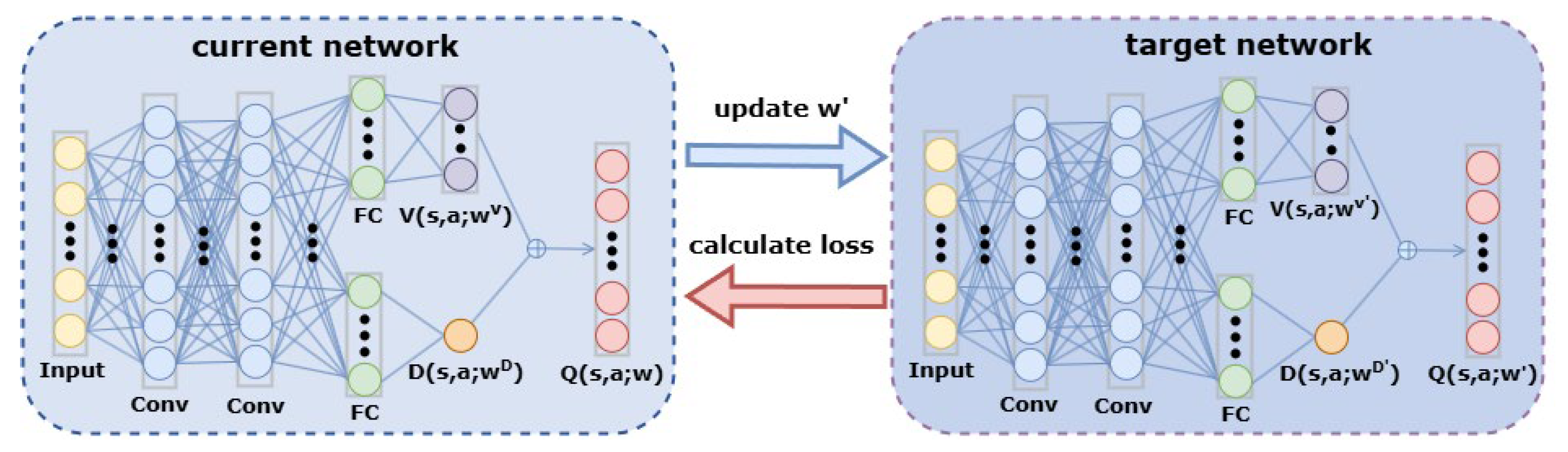
As shown in
Figure 3, the PODQN algorithm introduces a target network to address the overestimation issue. It does not solely rely on the estimated value of the current network to select actions and calculate their values.
First, the action
with the highest action-value is selected by the current network
, as shown in Equation (11):
Then, the target action-value
is calculated using the target network. The neural network structure of the target network is identical to that of DQN, but it has different parameters
. The calculation formula is given by Equation (12):
In contrast, the PODQN algorithm uses two networks for action selection and evaluation, reducing the positive bias caused by estimating the maximum return using the same network. Since the update process alternates between two networks, even if either network overestimates the value of an action, the effect of this overestimation will be corrected through the update of the other network, reducing the cumulative error caused by overestimation.
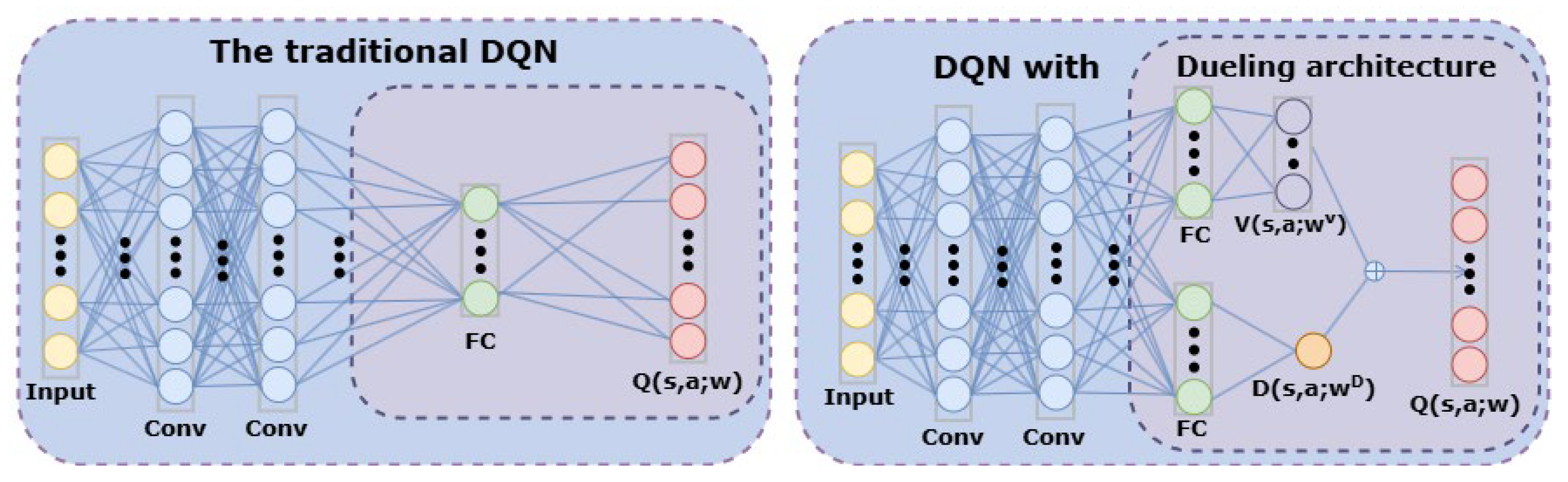
4.2. Dueling Network
Algorithms of the DQN type require calculating the action-value Q for each action. However, only the maximum action-value Q is needed for most states. The PODQN algorithm addresses this issue by decomposing the action-value function into the state value function and the advantage function. Without altering the input and output of the network, the architecture is optimized to better understand the value of states and the advantages of different actions, achieving more stable and efficient learning.
Figure 4 illustrates the changes if dueling architecture is introduced. The formula of advantage function
is expressed in Equation (13):
where
represents the action-value for state
and action
as calculated by the policy function
.
represents the state-value for state
if the policy function is
, which also represents the average of
across all actions.
Therefore, the advantage function illustrates the advantage of a specific action in comparison to the average value. If the advantage value of an action is the greatest, it signifies that the return obtained by performing this action will be higher than others. Although the actual values of the advantage function and the action-value function differ, the optimal action can be obtained through the advantage function only, resulting in reduced computation. By transforming the previous expression, Equation (14) shows the action-value function output by the PODQN algorithm:
In the PODQN algorithm, two neural networks
and
are used to approximate the optimal advantage function and the optimal state-value function respectively. By substituting
and
in the previous formula with the corresponding neural networks, the optimal action-value function Q is approximated according to Equation (15):
Nonetheless, these networks exhibit non-identifiability.
and
can vary freely without altering the output Q value, leading to unstable parameters during training and ineffective convergence. To promote the stable training without changing the output, a constant zero term
is added. As defined in Equation (16), the expression for the action-value function output by the PODQN algorithm is updated to:
where
represents the action space of this environment. The reasoning process for
being constantly zero is shown in Equation (17):
In practical applications, employing the average value for calculations often results in a more stable model than using the maximum value. As defined in Equation (18), the formula for computing Q-values is:
4.3. Gated Recurrent Unit
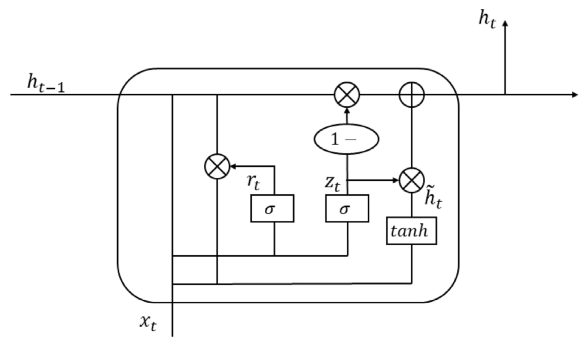
Since the sensors carried by UAVs have fixed sensing ranges and capabilities, each UAV can only collect information within the coverage range of its sensors. Collaboration of multi-UAV also typically covers only a small portion of the search area. This limitation makes it impossible to accurately evaluate the value of each action based only on a small part of the whole status. To overcome this problem, a feasible strategy is to let UAVs memorize past observation data and utilize all available information to make decisions. It can gradually enhance the overall understanding of the environmental state and make policy more rational. Recurrent Neural Network (RNN) is introduced to remember previously observation information.
Among RNN and its variants, Gated Recurrent Unit (GRU) is adopted for below advantages. Compared with traditional RNNs, GRU offers improved gradient flow mechanisms which can alleviate the gradient vanishing problem in long-term data sequences. While Long Short-Term Memory (LSTM) is commonly used to address vanishing or exploding gradients, GRU merges the forget gate and the input gate into an update gate, offering a simpler structure with fewer parameters, resulting in reduced computational costs and faster training. This property is beneficial for real-time UAV target search tasks, where both rapid evaluation and time-sensitive responses are crucial.
Furthermore, the dimension of GRU’s hidden layer is set to 64 based on preliminary experiments balancing representation capability and computational efficiency. Smaller hidden size is insufficient to capture complex spatiotemporal relationships in UAV search scenarios, whereas significantly larger dimensions increased model complexity and training times without yielding substantial improvements in accuracy or stability. Hence, the 64-dimensional hidden layer reflects a well-founded tradeoff between performance and resource constraints. The architecture of GRU is shown in
Figure 5.
The GRU layer adopts a gating mechanism to manage the long-term memory and short-term updating of information. It mainly contains update gate and reset gate. Update gate is used to control the extent to which the hidden state from previous timestep is retained at the current timestep, preserving long-term dependencies within the sequence. Its expression is shown in Equation (19):
where
and
are the weight and bias terms of the update gate.
represents the sigmoid activation function.
is the hidden state of the previous timestep.
is the input for the current timestep.
The reset gate is used to combine the latest input information with the observation information from the previous timestep, capturing short-term dependencies in the sequence. Its expression is shown in Equation (20):
Among them, and are the weight and bias terms of the reset gate. GRU regulates the flow of information through update gates and reset gates so the model can effectively learn useful information from the sequence of observation data and maintain the memory of past behaviors.
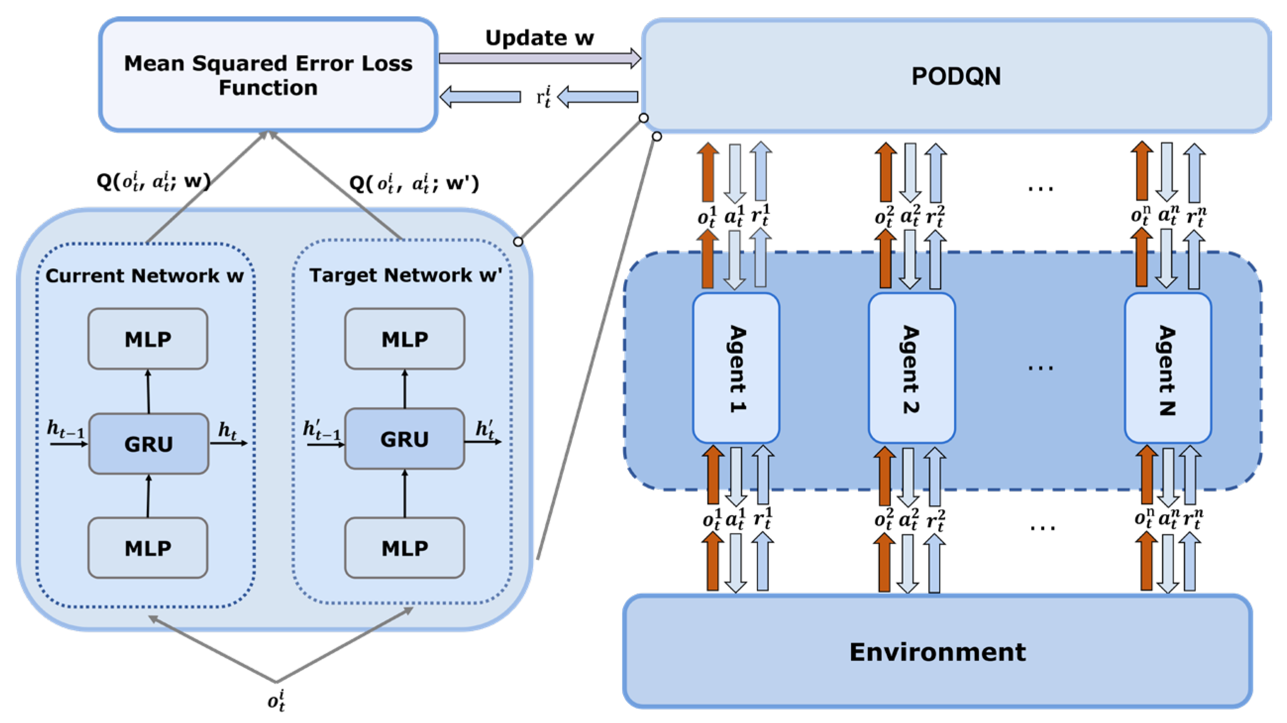
4.4. Multi-Agent Framework for the PODQN Algorithm
To implement the cooperation of UAVs in target search missions, a shared network is used to train all UAVs. Each UAV inputs its interaction information with the environment into the shared network and selects its action based on the output. The behaviors and learning experiences of all UAVs are fed back to the same network, allowing each UAV to further optimize the policy based on the behaviors of other UAVs and promoting the collaborative efficiency of the entire swarm. In addition, all UAVs sharing the same network can eliminate the need for independent tuning of each agent during the training process, reducing the overall number of parameters and accelerating the learning process of the system.
Figure 6 clearly depicts the relationship between each agent and the shared network. Each UAV transmits real-time data to the shared network. The network analyzes the observation data and returns corresponding actions to guide the UAV in its search. Then, the UAV provides the reward obtained by performing the selected action to the system for updating the network parameters. Through this method, the UAV swarm can achieve close collaborative search while maintaining autonomy, significantly improving search efficiency and accuracy.
Based on the above method, the hierarchical structure of the PODQN algorithm is shown in
Figure 7. In this structure, two convolutional layers with the ReLU activation layer extract features from the input observation state. Two linear layers map the feature vector to the input dimensions of the GRU layer, solving the problem of insufficient information caused by incomplete observations. The subsequent linear layer integrates the time-dependent features output by the GRU layer into a fixed-size vector, which serves as the input of the State Value stream and Action Advantage stream in the dueling architecture.
The State Value stream outputs a real number, indicating the state’s expected return. The Action Advantage stream outputs a vector with the same dimensions as the action space. Each dimension represents the advantage value of the corresponding action. By adding the outputs of two streams, the value of each action in this state can be calculated. Next, the model would choose an action through the action selection strategy.
4.5. Action Selection Strategy
During the network training process, always choosing the action with the greatest value to perform will lead the approximated value function to fall into local optimum if collected sample is biased. The ε-greedy strategy is used to balance whether the UAV should explore or use known information to select actions. There is a hyperparameter
that determines the balance between exploration and exploitation
In the later stages of training, the model has approximated the optimal policy through extensive trials so it can accurately evaluate the potential value of each action. Continuing random exploration at this stage may cause the model to deviate from the efficient policy that has been found. So, the annealing strategy is used to gradually decrease the value of
as the training epochs increase. The decay function is defined in Equation (20).
where
is the lowest limit to which
can decay and
is the decay speed of
. In the early stages of training, model needs to try unknown actions to explore the environment. As training progresses, model can evaluate the rewards of different behaviors to gradually approximate the optimal policy.
is also appropriately decreased. To prevent the model from prematurely converging to the local optimum and ignoring other potentially useful states,
ensures the model retains some exploratory capability in the later stages of training.
4.6. Artificial Potential Field
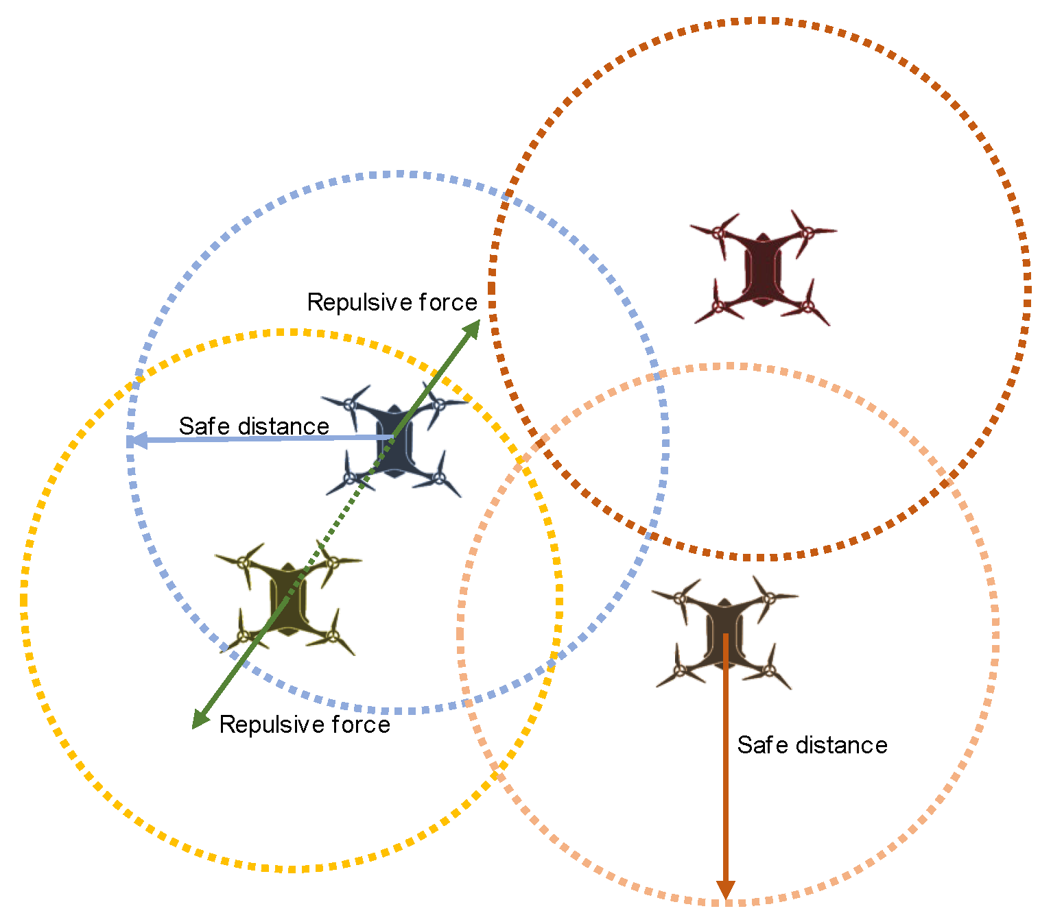
In unknown search environments, each UAV needs to dynamically adjust its flight path based on real-time information about the surrounding environment to avoid other UAVs. The artificial potential field method is a collision avoidance method based on physical mechanics. It treats each UAV as a particle subject to potential forces exerted to it. Each UAV calculates the vector superposition of all the forces it receives in the potential field, and it moves under the effect of the resultant force, achieving the autonomous movement with collision avoidance.
Figure 8 presents the repulsive force between UAVs.
In the repulsive potential field, the repulsive potential is emitted from each UAV and the potential force can be divided into two parts. If the distance between UAVs is longer than the prescribed safe distance
, the potential force would be 0. As the UAVs continue to fly, the repulsive force is inversely proportional to the distance if the distance between two UAVs is less than
. At each moment, all repulsive forces experienced by each UAV are calculated and resolved into x and y axes to update the UAV’s position. The distance between UAVs is calculated by the Euclidean distance and Equation (23) shows the potential field function.
In this formula, represents potential force factor and represents the flight speed of the UAV. In practical applications, the configuration of hyperparameters needs to be adjusted according to the needs of specific application scenarios. is the key factor in determining the threshold for triggering repulsive forces. In the case of high flight speed and large size of the UAV, appropriately increasing can extend the reaction time to avoid collision. Conversely, can be appropriately lower if the UAV is equipped with sensors with wide detection ranges and high accuracy. Its excellent perception ability enables it to detect obstacles in advance and avoid them in time.
In addition, is used to adjust the intensity of the repulsive force. In scenarios where perception accuracy is lower or communication latency exists, a higher is required to avoid collisions. However, excessively large may result in unnecessary deviations in flight paths, leading to additional search distance and energy consumption. For non-emergency tasks, reducing can enhance the stability and continuity of the flight path.
4.7. Algorithm Process
The pseudocode of this algorithm is shown in Algorithm 1 and the following are the steps for running the PODQN algorithm:
- (1)
Initialization: Before starting training, the parameters of the current network, the parameters of the target network, and the experience replay buffer should be initialized. The experience replay buffer is used to store observations, actions and rewards. Then, jump to the start state of environment and store the information in the experience replay buffer.
- (2)
Select action : At each moment, each agent can select the action based on the ε-greedy strategy.
- (3)
Obtain environmental feedback: After the action is executed, the UAV would receive the new state and the reward .
- (4)
Update the experience replay buffer: store the experience replay array (, , , ) into the experience replay buffer. If the experience replay buffer overflows, the latest experience will be used to replace the initially stored experience.
- (5)
Update the current network parameters: randomly sample a batch of samples from the experience replay buffer and calculate the TD error
:
Among them,
represents discount factor.
- (6)
Backpropagation: Calculate the gradient
and use the gradient descent method to update the parameters of the current network
. Equation (25) presents the formula for updating parameters:
where
represents the learning rate.
- (7)
Update target network parameters
: To enhance the stability during the training process, the soft update method is used to make the parameters of the target network slightly closer to the parameters of the current network each time it is updated. The soft update formula is given by Equation (26):
where
represents the soft update factor.
- (8)
Iteration: Repeat steps 2–7 until the maximum training epoch is reached.
| Algorithm 1: The pseudocode for the training process of the PODQN algorithm. |
| Input: Training parameters: learning rate , discount factor , experience replay buffer D, training period , soft update factor |
| Output: Action-value |
1. Initialize the parameters w, w′ of the current network Q(o, a; w) and the target network Q′(o, a; w′)
2. Initialize the experience replay buffer D and the parameter ε for annealing ε-greedy strategy
3. For episode 1 to do
4. Reset the environment and observe the initial state o1
5. While observation ot is not the terminal do
6. Calculates the action with the highest Q-value in action space based on the observation ot by the current network
7. Select an action at using the annealing ϵ-greedy strategy
8. Execute action at, obtain reward rt and observe the new state 0t+1
9. Store (ot, at, rt, ot+1) into experience replay buffer D
10. Randomly sample experience data from experience replay buffer D
11. Calculate the target action-value
12. Calculate the Mean-Square Error loss function
13. Calculate gradient
14. Update the parameters of the current network w to minimize the loss function:
15. Update the parameters of the target network by soft updating:
16. End while
17. End for |
5. Experiments and Discussions
RL requires agents to interact with the environment to obtain training data instead of using pre-prepared datasets. To verify the effect of the approach, a simulation environment is established to simulate realistic search scenarios.
Table 1 details the hyperparameter settings of the PODQN model. The configuration of each hyperparameter should comprehensively consider the computational complexity, feature extraction capabilities, and model convergence performance to ensure that the model has good adaptability and robustness in multi-UAV collaborative search tasks. Parameter configurations are determined based on tuning experience and preliminary experiments to balance the model performance with computational cost.
Through multiple preliminary experiments results, it was found that the convolution layers with given hyperparameters can effectively capture the input environmental information. Further changing the convolution size would significantly increase the training time while the improvement in searching is relatively limited. The current settings of network sufficiently meet the need of feature extraction. Further adjustments on it may lead to redundant calculations and even introduce the overfitting problem. The 64-dimensional hidden layer is able to ensure the accurate policy while achieving fast training convergence speed and low memory consumption. It can capture effective temporal features without excessively increasing model complexity. The parameters of the ϵ-greedy strategy were also validated through experiments, ensuring the agent maintains broad exploration in the early stages and gradually shifts to exploiting accumulated experience as training progresses. The learning rate and soft update factor showed good convergence stability in preliminary experiments.
The simulation environment is a limited search area based on a search map with a size of 50 × 50. All UAVs are assumed to search at the same altitude and at a constant speed. The direction of the UAV is determined by changing the yaw angle by executing actions in the action space. When the distance between the UAVs falls below the effective range of the repulsive field, the resulting repulsive force would compel each UAV to move in the direction opposite to the other UAV’s position. The observation data collected by each UA consist of its coordinates, yaw angle, and the number of targets within its observation range. The condition for a target to be successfully found is that the distance between the target and the UAV is less than the observation range. To prevent unbounded search, a fixed search time limit is set in the experiment. Each episode would terminate once all UAVs reach this time limit or once all targets have been found.
Table 2 presents the hyperparameters configured for the experiment.
The number of targets is set to 15 and the position of each target will be appropriately adjusted according to its determinacy for simulating the situation in which the target position is biased or updated late in reality. The coordinates of the determined target will be imported directly from the specified file. For undetermined targets, their coordinates will change randomly based on the provided fuzzy position to simulate possible position deviations.
Table 3 lists the certainty of the targets and the corresponding coordinates mapped to the map in detail.
Three, four, and five UAVs are selected as experimental objects to reflect the collaboration of multi-UAV. Each evaluation matrix is obtained by randomly generating 20 rounds in each training cycle and taking the average, reducing the impact of randomness in one round and reflecting the performance reliably.
5.1. Scenario I: Three UAVs
Figure 9a,b show the training process of the proposed PODQN algorithm, DQN, Double DQN, Dueling DQN, Value Decomposition Network (VDN), QMIX and random policy. As can be seen from curves, the reward of random search algorithm is kept near a low value, indicating it is difficult to optimize according to the feedback from the environment. The number of targets found by the DQN algorithm fluctuates significantly over time. Although it can occasionally find more targets, the overall performance lacks consistency and the found targets is close to zero in some training stages. Similarly, the corresponding reward curve frequently experiences reward declines and intervals of negative rewards with the overall trend failing to demonstrate a continuous increase. For Double DQN, the average number of targets found is higher than 10 during most of the training period, while the reward curve experiences sharp fluctuations many times throughout the training process and more than half of the reward values are below 0. The overall performance fluctuation of the Dueling DQN algorithm is the largest and there is a large performance gap even between adjacent training epochs. When training to about 54,000 epochs, its reward value stabilizes at about −1800, indicating that the algorithm has not found an effective search strategy. The performance of VDN is not stable during the learning process. Although it can find more targets sometimes, the overall stability is poor and the curve fluctuates significantly, which indicates that VDN is easily affected by environmental changes. In contrast, QMIX found more targets than the previous algorithms. However, it can be seen from its reward curve that most of the reward values are still below 0. Even if some targets are successfully found, the search path still needs to be further optimized. Compared with other algorithms, the PODQN algorithm can find more targets in most periods with obvious peak values and small changes, showing best performance. A more intuitive comparison can be obtained from
Table 4.
5.2. Scenario II: Four UAVs
Figure 9c,d show the training process of different algorithms under four UAVs. The random policy shows significant performance deficiencies. Its reward value hovers in the negative area in most cases and fluctuate around −470. While higher rewards may occasionally be obtained, this is an accidental result of randomness rather than a stable performance of the algorithm. The DQN algorithm is capable of finding more than 10 targets in certain stages, but it would abruptly decline to a low level or even drop to 0. Meanwhile, its reward curve exhibits repeated fluctuations over time with a significant improvement around 80,000 epochs followed by a decrease back to approximately −3000. This oscillatory behavior between high and low performance indicates that the policy is not yet stable and has not achieved steady convergence. The Double DQN algorithm remained relatively stable until the last 20,000 epochs. Its reward curve showed a downward trend from nearly 1000 to around −900 and never recovered to a positive value. The Dueling DQN algorithm was able to find 12 to 13 targets before training to approximately 32,000 epochs. But its search policy changed rapidly, resulting in it only being able to find 1 target in subsequent training. Although it occasionally recovered to the level of finding 12 targets, this phenomenon was not sustained, and it would return to the poor performance in the following epoch. The VDN algorithm once found all the targets. However, its reward fluctuates around −260 in most training epochs. This may be because it fell into a local optimal solution and there was no further strategy adjustment. The QMIX algorithm is highly volatile throughout the training process and does not have an obvious upward or downward trend. The number of discovered targets and the reward frequently alternate between peaks and troughs, indicating its erratic performance. Only the PODQN algorithm has an overall upward trend. Even though it fluctuates in some stages, it would recover quickly and remain at a high level in most stages, showing the excellent overall performance.
5.3. Scenario III: Five UAVs
Figure 9e,f show the training process under five UAVs. The random policy is relatively flat and has a small fluctuation range. The reward keeps fluctuating around 0 throughout the training process, staying at a low level. The DQN algorithm has obvious stage peaks with the number of targets consistently maintained between 8 and 12 in specific training intervals such as 20,000 to 30,000 epochs. Then, it would decline to a low number of targets and a negative reward range of approximately −3000 to −3500. DQN has learned some high-value action sequences under the current training settings, but it lacks continuous reinforcement of this policy. The Dueling DQN algorithm shows the largest fluctuations in the curve of found targets, demonstrating significant performance differences between two close epochs. Additionally, the reward curve generally shows a declining trend, occasionally spike briefly before quickly dropping below −3000. In contrast, the Double DQN algorithm shows strong search performance initially. But it experiences a steep decline at about 68,000 epochs with the reward falling below −700. After this turning point, curves rise a little but the reward remains stable at less than 0. The VDN algorithm is similar to the Double DQN algorithm. Although the number of targets found in the later stage is stable around 14, its rewards show that its search path needs to be further optimized. The performance of the QMIX algorithm seems to be relatively stronger from
Figure 9e. But the reward exhibits fluctuations exceeding 2000 starting from 21,000 epochs. The PODQN algorithm has similar performance and small fluctuation most of the time. However, its peak value is larger and has stabilized in the last 10,000 epochs, indicating the most reliable performance.
Combined with the above analysis, it is not difficult to conclude that the proposed PODQN algorithm displays stable performance and remarkable convergence. When extended to multi-agents, its performance is also better than various DQN-based algorithms and commonly used algorithms, which can maintain stable performance gains even as the number of agents increases.
5.4. Multi-UAV Collaborative Analysis
Figure 10a,b present the performance of the PODQN algorithm under three different numbers of UAVs. It can be observed that the PODQN algorithm shows significant performance and convergence on evaluation metrics as the number of UAVs increases. When the number of agents is 3, the PODQN algorithm demonstrates a rapid convergence speed and a high cumulative reward, indicating that it can quickly find effective collaborative strategies in smaller-scale multi-agent systems. When the number of UAVs increased to four and five, despite large fluctuations in the early stages of training due to policy adjustments brought resulting from environmental exploration, its convergence speed still maintains a high level and the number of found targets also maintains a stable and gradual increase, highlighting the robust adaptability and scalability involving a greater number of UAVs. Additionally, the stability of the strategy is not largely affected as the number of UAVs increases, indicating that the PODQN algorithm can effectively mitigate policy oscillations in multi-UAV collaboration tasks and improve the efficiency.
However, this study only addresses cases involving three, four, and five UAVs. When the scale of UAVs further expands to dozens or hundreds, the linear or even exponential growth of state space and action space caused by the increase in the number of agents will lead to a significant increase in the complexity of policy optimization. In this context, the performance may level off or even cause bottlenecks in some cases. To reduce the computational cost of the PODQN algorithm and speed up the convergence speed in large-scale UAV systems, a hierarchical learning framework can be introduced based on the existing shared network framework to divide the large-scale UAV swarm into several sub-groups. Each subgroup independently learns policies within its local scope and makes collaboration among subgroups through the global level. Furthermore, deploying a distributed framework can accelerate training by distributing the processing of large-scale training data across different nodes. Each UAV can independently interact with the environment and sample experience. This distributed mechanism can not only train networks of different modules at the same time to improve the convergence speed but also enhance the scalability of the algorithm in more complex task environments.
6. Conclusions
In general, this paper aims to achieve dynamic and adaptive target search for UAVs through reinforcement learning. Considering the limitations of UAVs in observing the environment, this paper proposes the PODQN algorithm to solve its partially observable problem in practical applications. First, the target search task is modeled as a partially observable Markov Decision Process and an innovative reward function is designed for different search scenarios. Subsequently, the network architecture of the PODQN algorithm is introduced in detail and extended to multi-agent systems. Through experiments in simulation environments and comparative analysis with other algorithms, the PODQN algorithm shows stronger stability and better performance under different numbers of UAV configurations.
Although the constructed simulation environment has accounted for as many real-world factors as possible, it cannot fully replicate the complexity and random disturbances of real-world scenarios. For this reason, future work would focus on introducing practical factors such as noise caused by sensor errors and communication delays. Additional consideration would be given to uncontrollable environmental disturbances, including wind field perturbations and terrain interference. By deploying and testing the algorithm on more realistic UAV platforms, the robustness and feasibility of the system can be further evaluated under more complex perception and communication conditions, which would contribute to providing a more comprehensive solution for the deployment of multi-UAV cooperative search in real-world scenarios.


