Distributed Constrained Optimization Algorithms for Drones

Abstract

The present study addresses a critical issue within the realm of drones: the challenge of distributed constrained optimization. Our research delves into an optimization scenario where the decision variable is confined to a closed convex set. The primary objective is to develop a distributed algorithm capable of tackling this optimization problem. To achieve this, we have crafted distributed algorithms for both balanced graphs and unbalanced graphs, with the method of feasible direction employed to address the considered constraint, and the method of estimating left eigenvector to address the unbalance, incorporating momentum elements. We have demonstrated that the algorithms exhibit linear convergence when the local objective functions are both smooth and strongly convex, and when the step-sizes are appropriately chosen. Additionally, the simulation outcomes validate the efficacy of our distributed algorithms.

1. Introduction

Recently, distributed optimization has emerged as a significant research area in drones, leading to substantial advances. During past years, although several attempts were made to employ distributed optimization algorithms to address the decision problems involved in drones (see [1,2]), their usage in multi-robot systems is still limited to only a handful of examples, as discussed in [3]. On the other hand, it is also mentioned in [3] that many problems, including multi-robot target tracking, cooperative estimation, distributed simultaneous localization and mapping, and collaborative motion planning in multi-robot coordination and collaboration, can be formulated and solved within the framework of distributed optimization. Therefore, in this paper, we focus on designing novel distributed optimization algorithms and explore their potential applications in drones.

Recently, numerous influential results of distributed optimization have been achieved in this domain, encompassing both continuous-time distributed optimization algorithms (see [4,5,6,7,8,9,10,11]) and discrete-time distributed optimization algorithms (see [12,13,14,15,16,17,18,19,20,21,22,23,24,25,26,27,28,29,30]). Notably, significant attention has been attracted by distributed constrained optimization, particularly with discrete-time algorithms designed for closed convex set constraints.

Initially, research primarily centered on distributed optimization algorithms that employed nonnegative decaying step-sizes, leading to algorithms with sub-linear convergence rates. The earliest studies addressed unconstrained optimization problems, with distributed algorithms over balanced graphs developed in [12]. Subsequent work expanded these methods to include closed convex set constraints in [13] and global general constraints in [14]. When fixed unbalanced graphs were considered, distributed algorithms were developed to handle optimization problems with N non-identical set constraints in [15] and those with additional equality and inequality constraints in [16]. Under time-varying unbalanced graph sequences, the Push-sum framework facilitated the design of distributed algorithms for unconstrained optimization in [17], while an improved push–pull framework enabled solutions to problems with equality constraints and set constraints in [18].

More recent efforts have emphasized the design of distributed optimization algorithms achieving linear convergence rates. In [19], a distributed algorithm over balanced graphs was developed for unconstrained optimization, while further studies addressed the case of fixed unbalanced graphs in [20,21,22]. For time-varying unbalanced graphs, the Push-DIGing algorithm and a push–pull-based algorithm were proposed in [23,24]. These methods, however, are limited to solving unconstrained optimization problems. For constrained cases, an algorithm over a fixed unbalanced graph was developed for problems with a closed convex set constraint in [25].

Then, for further accelerating the convergence of the designed algorithms, the momentum terms were introduced in the proposed distributed optimization algorithms in [27,28,29], where only the unconstrained optimization problems were studied. Moreover, the approach of employing momentum terms was later extended in the case with a global closed convex set constraint in [30]. Although the momentum-based algorithm in [30] achieves linear convergence, its use of dual iterative scales adds computational complexity. Thus, this paper aims to design novel distributed optimization algorithms for solving the constrained optimization problem with only one iterative scale and thus with lower computational complexity.

This paper’s main contribution lies in proposing the distributed optimization algorithms with linear convergence and momentum terms for problems with a global closed convex set constraint. Utilizing the method of feasible directions to handle the constraint, this approach eliminates the need for the dual iterative scales used in [30], thus reducing computational complexity.

We structure the remainder of the paper as follows. Section 2 introduces the relevant notations, graph theory, and matrix theory. Section 3 presents the decision problem of drones, the proposed distributed algorithm, the main theorem, and a detailed convergence analysis. In Section 4 and Section 5, the results of simulation and conclusions are given, respectively.

2. Preliminaries

2.1. Notations

In this paper, the n-dimensional real vectors set is denoted by the ${\mathbb{R}}^n$. Especially, $\mathbf{1}$ denotes the vectors with a proper dimension and all entries being 1. Let $x\in {\mathbb{R}}^n$ be a vector; $x^i$ denotes its i-th entry, and $x^T$ denotes its transpose. Moreover, $\parallel x\parallel$ stands for its 2-norm. Especially, if all $x^i$, $i=1,2,\cdots ,n$ are positive (non-negative), x is called positive (non-negative). Moreover, ${\mathbf{e}}_i$ stands for the vectors with a proper dimension and with its i-th entry being 1 and other entries being 0. Additionally, for a function $f\left(y\right)$ defined on ${\mathbb{R}}^n$, $\nabla f\left(x\right)$ represents the gradient of f at x. Let ${\mathbb{R}}^{m\times n}$ denote the $m\times n$-dimensional real matrices set. Especially, $I_N$ denotes the real identity matrix with a proper dimension. Let $M\in {\mathbb{R}}^{m\times n}$ be a matrix; its transpose and the 2-norm induced matrix norm are, respectively, denoted by $\parallel M\parallel$ and $M^T$. Moreover, its $ij$-th is denoted by $M_{ij}$. Especially, if all $M_{ij}$, $i=1,2,\cdots ,m$, $i=1,2,\cdots ,j$ are positive (non-negative), M is called positive (non-negative). Moreover, for a closed convex set $X_0\subseteq {\mathbb{R}}^n$ and a vector w, $P_{{\Omega }_0}\left(w\right)$ denotes the projection of w on $X_0$.

2.2. Graph Theory

In this paper, the notations and definitions associated with the graph are the same as those described in [25] and thus are omitted here.

2.3. Matrix Theory

This subsection gives the definition of doubly stochastic matrices and the significant results of doubly stochastic matrices and non-negative matrices.

Definition 1.

Let $A\in {\mathbb{R}}^{N\times N}$ be a non-negative matrix. A is called a non-negative stochastic matrix if $A\mathbf{1}=\mathbf{1}$. Moreover, A is called a non-negative doubly stochastic matrix if $A\mathbf{1}=\mathbf{1}$ and ${\mathbf{1}}^{T}A={\mathbf{1}}^T$.

Lemma 1

([31,32]). Let $A\in {\mathbb{R}}^{N\times N}$ be a non-negative doubly stochastic matrix associated with the strongly connected directed graph $\mathcal{G}$. Especially, for all $1\le i\le N$, suppose that $A_{ii}>0$ are positive. Then, we have $\parallel A-{\displaystyle \frac{1}{N}}\mathbf{1}{\mathbf{1}}^T\parallel \le \rho$, with $0<\rho <1$ being a constant.

Lemma 2

([32]). For a non-negative matrix $G\in {\mathbb{R}}^{n\times n}$, if $G\delta <\theta \delta$ holds for a positive constant θ and a positive vector $\delta \in {\mathbb{R}}^n$, then $\parallel G\parallel <\theta$.

3. Main Results

We will give the decision problem of drones, the proposed distributed algorithm and main theorem, and the convergence analysis in this section.

3.1. Decision Problem of Drones

In recent years, drones have seen significant application across various practical fields such as the military, terrain exploration, and power grid fault detection. As multi-scenario tasks become more complex, task completion often requires the coordination of multiple drones. Due to the lengthy time required and the lack of robustness in solving large-scale optimization problems, centralized optimal decision-making methods cannot meet the intelligent demands of multi-drone clusters for handling complex tasks. Consequently, distributed optimization algorithms are increasingly employed to enable efficient autonomous decision-making in multi-drone clusters. For instance, in terrain exploration tasks, the influence of complex terrain requires that multi-drone clusters consider not only their inherent optimization objectives but also the impact of terrain constraints on drone actions. Therefore, the autonomous decision-making problem for multi-drone clusters can be formulated as the following mathematical model:

$$\begin{array}{c}\hfill \underset{k}{min}h\left(k\right)={\displaystyle \frac{1}{N}}\sum _{i=1}^N{h}_i\left(k\right)\mathrm{s}.\mathrm{t}.k\in K_0,\end{array}$$

(1)

where $h_i:{\mathbb{R}}^m\to \mathbb{R}$ is the convex function representing the optimization objectives of drones and $K_0\subseteq {\mathbb{R}}^m$ is a set being convex and closed standing for the constraint observed by drones. As discussed in [25], for a optimal solution $k^{*}$ to problem Equation (1), it holds that

$$k^{*}=P_{K_0}(k^{*}-{\nu }_0\nabla h\left(k^{*}\right)),$$

(2)

with ${\nu }_0$ being an arbitrary positive constant. Especially, let $m=1$ in the subsequent analyses for convenience, and the case with $m>1$ has been discussed in detail in [25].

In the following, we first give a necessary assumption for problem Equation (1), which is standard and usually introduced in the works researching the distributed optimization algorithms having linear convergence.

Assumption 1.

All $h_i$ are L-smooth and α-strongly convex on ${\mathbb{R}}^m$, where α and L are positive constants.

3.2. Proposed Distributed Algorithm and Main Theorem

In this subsection, the distributed optimization algorithm is designed on the strongly connected balanced graph $\mathcal{G}$, and the main theorem about the proposed algorithm owing linear convergence is given.

Especially, motivated by [26,30], the discrete-time distributed algorithm is designed as in Algorithm 1, where $k_i\left(a\right)\in {\mathbb{R}}^m$ is the estimation on the optimal solution of node i at a; A is the weighted matrix associated with $\mathcal{G}$, which is assumed to be non-negative doubly stochastic; $l_i\left(a\right)\in {\mathbb{R}}^m$ is the estimation on the gradient of h of node i at a; and $\alpha$, $\beta$, and $\eta >0$ are fixed step-sizes. Especially, $k_i\left(0\right)$ can be arbitrarily selected in ${\mathbb{R}}^n$ and $l_i\left(0\right)=\nabla h_i\left(k_i\left(0\right)\right)$.

Algorithm 1: Distributed Algorithm over Balanced Graph

I: Input: $\alpha >0$, $\beta >0$, $\eta >0$, N, A;  II: Initialize: For all i, $k_i\left(0\right)=k_i(-1)\in {\Re }^m$, $r_i\left(0\right)=\nabla h_i\left(k_i\left(0\right)\right)\in {\Re }^m$;  III: Iteration rule: $$k_i(a+1)=\sum _{j=1}^N{A}_{ij}{k}_j\left(a\right)+\eta e_i\left(a\right)+\beta d_i\left(a\right),$$ (3) $$l_i(a+1)=\sum _{j=1}^N{A}_{ij}{l}_j\left(a\right)+r_i\left(a\right),$$ (4)  with $$\begin{array}{cc}\hfill e_i\left(a\right)& =k_i\left(a\right)-k_i(a-1),\hfill \\ \hfill d_i\left(a\right)& =P_{B_0}\left(k_i\left(a\right)-{\displaystyle \frac{\alpha }{\beta }}{l}_i\left(a\right)\right)-k_i\left(a\right),\hfill \\ \hfill r_i\left(a\right)& =\nabla h_i\left(k_i(a+1)\right)-\nabla h_i\left(k_i\left(a\right)\right).\hfill \end{array}$$  VI: Output

For rewriting Equation (3) in compact form and thus the convenience in the subsequent analysis, we introduce the following variable:

$$\begin{array}{cc}\hfill \mathbf{k}\left(a\right)& ={(k_1\left(a\right),k_2\left(a\right),\cdots ,k_N\left(a\right))}^T,\hfill \\ \hfill \mathbf{l}\left(a\right)& ={(l_1\left(a\right),l_2\left(a\right),\cdots ,l_N\left(a\right))}^T,\hfill \\ \hfill \mathbf{d}\left(a\right)& ={(d_1\left(a\right),d_2\left(a\right),\cdots ,d_N\left(a\right))}^T,\hfill \\ \hfill \mathbf{e}\left(a\right)& ={(e_1\left(a\right),e_2\left(a\right),\cdots ,e_N\left(a\right))}^T,\hfill \\ \hfill \nabla \mathbf{H}\left(\mathbf{k}\right(a\left)\right)& ={(\nabla h_1\left(k_1\left(a\right)\right),\cdots ,\nabla h_N\left(k_N\left(a\right)\right))}^T,\hfill \end{array}$$

and $K=K_0^N$. Then, we can rewrite Equation (3) as

$$\begin{array}{cc}\hfill \mathbf{k}(a+1)& =A\mathbf{k}\left(a\right)+\eta \mathbf{e}\left(a\right)+\beta \mathbf{d}\left(a\right),\hfill \end{array}$$

(5a)

$$\begin{array}{cc}\hfill \mathbf{l}(a+1)& =A\mathbf{l}\left(a\right)+\nabla \mathbf{H}\left(\mathbf{k}\right(a+1\left)\right)-\nabla \mathbf{H}\left(\mathbf{k}\right(a\left)\right).\hfill \end{array}$$

(5b)

Theorem 1.

With the feasible step-sizes α, β, and η, whose feasible regions are detailedly defined in the subsequent convergence analysis, for all $i,$ $k_i\left(a\right)$ under Algorithm 1 converge to the unique optimal solution to problem Equation (1) linearly under Assumption 1.

Proof. 

See Section 3.3 for the detailed proof. □

3.3. Convergence Analysis for Algorithm 1

The detailed convergence analysis of Algorithm 1 is shown in this subsection, with the strict proof of Theorem 1 given.

Moreover, we introduce several variables necessarily involved in the subsequent convergence analysis, which are defined as

$$\overline{k}\left(a\right)={\displaystyle \frac{1}{N}}{\mathbf{1}}^T\mathbf{k}\left(a\right),\overline{l}\left(a\right)={\displaystyle \frac{1}{N}}{\mathbf{1}}^T\mathbf{l}\left(a\right).$$

Lemma 3.

For Algorithm 1, one has

$$\begin{array}{cc}\hfill \overline{k}(a+1)& =\overline{k}\left(a\right)+{\displaystyle \frac{1}{N}}\eta \mathbf{e}\left(a\right)+{\displaystyle \frac{1}{N}}\beta \mathbf{d}\left(a\right),\hfill \end{array}$$

(6a)

$$\begin{array}{cc}\hfill \overline{l}(a+1)& ={\displaystyle \frac{1}{N}}{\mathbf{1}}^T\nabla \mathrm{H}\left(\mathbf{k}(a+1)\right)={\displaystyle \frac{1}{N}}\sum _{i=1}^N\nabla h_i\left(k_i(a+1)\right).\hfill \end{array}$$

(6b)

Proof. 

This proof is omitted here since it can be easily completed based on the proof of ([25] [Lemma 6]). □

Next, by introducing the variable as

$$\mathbf{x}\left(q\right)=\left(\begin{array}{c}\parallel \mathbf{k}\left(a\right)-\mathbf{1}\overline{k}\left(a\right)\parallel \\ \sqrt{N}\parallel \overline{k}\left(a\right)-b^{*}\parallel \\ \parallel \mathbf{e}\left(a\right)\parallel \\ \parallel \mathbf{l}\left(a\right)-\mathbf{1}\overline{l}\left(a\right)\parallel \end{array}\right),$$

we give a key lemma for establishing the linear convergence property of Algorithm 1.

Lemma 4.

Under Assumption 1 and when $0<{\displaystyle \frac{\alpha }{\beta }}<{\displaystyle \frac{2}{L}}$, there holds

$$\begin{array}{c}\hfill \mathbf{x}(a+1)\le G\mathbf{x}\left(a\right),\end{array}$$

(7)

where

$$\begin{array}{c}\hfill G=\left(\begin{array}{cccc}\rho +3\beta & 0& 2\eta & 2\alpha \\ \beta +\alpha L& \gamma & \eta & \alpha \\ 2+2\beta +\alpha L& 2\beta +\alpha L& \eta & \alpha \\ 2L(2+2\beta +\alpha L)& 2L(2\beta +\alpha L)& 2L\eta & \rho +2L\alpha \end{array}\right).\end{array}$$

Proof. 

See Appendix A for the detailed proof. □

In the following, the detailed proof of Theorem 1 is prepared.

Proof of Theorem 1.

Clearly, it is sufficient for completing the proof to select the feasible step-sizes $\alpha$, $\beta$, $\eta$ in order to make $\rho \left(G\right)<1$. Considering $0<{\displaystyle \frac{\alpha }{\beta }}<{\displaystyle \frac{2}{L}}$, we can select $\beta =2L\alpha$. Furthermore, noting Lemma 2, we can complete the proof by proving that there is a positive vector $\delta =[{\delta }^1,{\delta }^2,{\delta }^3,{\delta }^4]$ satisfying $G\delta <\delta$, i.e.,

$$\begin{array}{cc}\hfill {\delta }^1>& (\rho +3\beta ){\delta }^1+2\eta {\delta }^3+2\alpha {\delta }^4,\hfill \\ \hfill {\delta }^2>& (\beta +\alpha L){\delta }^1+\gamma {\delta }^2+\eta {\delta }^3+\alpha {\delta }^4,\hfill \\ \hfill {\delta }^3>& (2+2\beta +\alpha L){\delta }^1+(2\beta +\alpha L){\delta }^2+\eta {\delta }^3+\alpha {\delta }^4,\hfill \\ \hfill {\delta }^4>& 2L(2+2\beta +\alpha L){\delta }^1+2L(2\beta +\alpha L){\delta }^2+2\eta L{\delta }^3+(\rho +2\alpha L){\delta }^4.\hfill \end{array}$$

(8)

Then, substituting $\beta =2\alpha L$ into Equation (8), we can obtain

$$\begin{array}{cc}\hfill {\delta }^1>& (\rho +6\alpha L){\delta }^1+2\eta {\delta }^3+2\alpha {\delta }^4,\hfill \\ \hfill {\delta }^2>& 3\alpha L{\delta }^1+\gamma {\delta }^2+\eta {\delta }^3+\alpha {\delta }^4,\hfill \\ \hfill {\delta }^3>& (2+7\alpha L){\delta }^1+7\alpha L{\delta }^2+\eta {\delta }^3+\alpha {\delta }^4,\hfill \\ \hfill {\delta }^4>& 2L(2+7\alpha L){\delta }^1+14\alpha L^2{\delta }^2+2\eta L{\delta }^3+(\rho +2\alpha L){\delta }^4,\hfill \end{array}$$

(9)

which is equivalent to

$$\begin{array}{cc}\hfill 2\eta {\delta }^3<& (1-\rho -6\alpha L){\delta }^1-2\alpha {\delta }^4,\hfill \\ \hfill \eta {\delta }^3<& -3\alpha L{\delta }^1+(1-\gamma ){\delta }^2-\alpha {\delta }^4,\hfill \\ \hfill \eta {\delta }^3<& -(2+7\alpha L){\delta }^1-7\alpha L{\delta }^2+{\delta }^3-\alpha {\delta }^4,\hfill \\ \hfill 2\eta L{\delta }^3<& -2L(2+7\alpha L){\delta }^1-14\alpha L^2{\delta }^2+(1-\rho -2\alpha L){\delta }^4.\hfill \end{array}$$

(10)

Since $\eta$, ${\delta }^3$, and L are positive, if ${\delta }^1$, ${\delta }^2$, ${\delta }^4$, $\alpha$, and $\eta$ exist, which are positive constants, such that

$$\begin{array}{cc}\hfill 0<& (1-\rho -6\alpha L){\delta }^1-2\alpha {\delta }^4,\hfill \\ \hfill 0<& -3\alpha L{\delta }^1+(1-\gamma ){\delta }^2-\alpha {\delta }^4,\hfill \\ \hfill 0<& -(2+7\alpha L){\delta }^1-7\alpha L{\delta }^2+{\delta }^3-\alpha {\delta }^4,\hfill \\ \hfill 0<& -2L(2+7\alpha L){\delta }^1-14\alpha L^2{\delta }^2+(1-\rho -2\alpha L){\delta }^4,\hfill \end{array}$$

(11)

holds, positive constants ${\delta }^1$, ${\delta }^2$, ${\delta }^3$, ${\delta }^4$, $\alpha$, and $\eta$ exist such that Equation (10) holds. For arbitrary positive constant ${\delta }^3$, considering $\gamma =1-\mu \alpha$ with $\beta =2L\alpha$, we select ${\delta }^1=q_1{\delta }^3$, ${\delta }^2=q_2{\delta }^3$, and ${\delta }^3=q_3{\delta }^3$, with $q_1={\displaystyle \frac{1}{4}}$, $q_2={\displaystyle \frac{9}{4\mu (1-\rho )}}$, and $q_3={\displaystyle \frac{3}{2(1-\rho )}}$. Then, when

$$\begin{array}{c}\hfill \alpha <max\{{\displaystyle \frac{1-\rho }{6L+2q_3}},{\displaystyle \frac{1-2q_1}{7L{q}_1+7L{q}_2+q_3}},{\displaystyle \frac{L}{28L^2{q}_1+28L^2{q}_2+4L{q}_3}}\},\end{array}$$

(12)

Equation (11) holds. Then, with the selected $\alpha$, we can select

$$\begin{array}{cc}\hfill \eta <max\{& {\displaystyle \frac{(1-\rho )q_1-(6L+2q_3)\alpha }{2}},(-3L{q}_1+\mu q_2-q_3)\alpha ,\hfill \\ & (1-2q_1)-(7L{q}_1+7L{q}_2+q_3)\alpha ,\hfill \\ & {\displaystyle \frac{[(1-\rho )q_3-4L{q}_1]}{2L}},-{\displaystyle \frac{(14L^2{q}_1+14L^2{q}_2+2L{q}_3)\alpha }{2L}}\},\hfill \end{array}$$

(13)

to let Equation (10) hold. Therefore, the proof has been completed. □

3.4. Distributed Algorithm on Unbalanced Graph

It can be noted that in Section 3.2, we only consider the case that the communication graph between all drones is balanced, which means that any two directly connected drones (agents) can exchange information bidirectionally. However, in many cases that require privacy protection, the information exchange between two directly connected drones (agents) is unidirectional, which implies that the communication graph between all drones is unbalanced. Furthermore, it is difficult to design a nonnegative doubly stochastic matrix for an unbalanced graph, and a nonnegative stochastic matrix is always employed in the distributed optimization algorithms for cases involving the unbalanced graphs.

Accordingly, when matrix A is only the stochastic matrix, Algorithm 1 is ineffective to address the problem in Equation (1), and we will take the case without the constraint and without the momentum terms $e_i\left(a\right)$, for example, to explain the detailed reason. When the constraint and the momentum terms $e_i\left(a\right)$ are omitted, Algorithm 1 can be rewritten as

$$\begin{array}{cc}\hfill k_i(a+1)& =\sum _{j=1}^N{A}_{ij}{k}_j\left(a\right)-\alpha l_i\left(a\right),\hfill \end{array}$$

(14a)

$$\begin{array}{cc}\hfill l_i(a+1)& =\sum _{j=1}^N{A}_{ij}{l}_j\left(a\right)+r_i\left(a\right),\hfill \end{array}$$

(14b)

with the definition of $r_i\left(a\right)$ being the same as that in Section 3.2.

It is worth noting from Lemma 3 that $\overline{l}\left(a\right)$ can be approximatively seen as the gradient of the global objective function h at $\overline{x}\left(t\right)$ upon all $x_i\left(t\right)$ achieving consensus. Moreover, from the property of the non-negative doubly stochastic matrix as given in Lemma 2, we can obtain that all $x_i\left(t\right)$ achieve consensus linearly. Furthermore, for the consensus state $\overline{k}\left(t\right)$, we have

$$\begin{array}{cc}\hfill \overline{k}(a+1)& =\overline{k}\left(a\right)-\alpha \overline{l}\left(a\right),\hfill \end{array}$$

(15)

which can be approximatively seen as the classical gradient-decent iteration for obtaining the minimum of $h\left(k\right)$. Therefore, all $k_i\left(a\right)$ under Algorithm 1 will converge to the minimum of $h\left(k\right)$.

However, as discussed in [25], when A is only a non-negative doubly stochastic matrix, the result in Lemma 2 will become $\parallel A-{\displaystyle \frac{1}{N}}\mathbf{1}{\pi }^T\parallel \le \rho$ where $\pi$ is a nonnegative left eigenvector of A with respect to the eigenvalue 1, satisfying ${\mathbf{1}}^T\pi =N$. Then, we should re-define $\overline{k}\left(a\right)$ and $\overline{l}\left(a\right)$ as

$$\overline{k}\left(a\right)={\displaystyle \frac{1}{N}}{\pi }^T\mathbf{k}\left(a\right),\overline{l}\left(a\right)={\displaystyle \frac{1}{N}}{\pi }^T\mathbf{l}\left(a\right),$$

and can obtain that all $l_i\left(a\right)$ will converge to the consensus state $\overline{l}\left(a\right)$ and $\overline{l}\left(a\right)={\displaystyle \frac{1}{N}}{\pi }^T\nabla \mathrm{H}\left(\mathbf{k}(a+1)\right)={\displaystyle \frac{1}{N}}{\displaystyle \sum _{i=1}^N}{\pi }^i\nabla h_i\left(k_i(a+1)\right)$. Therefore, $l_i\left(a\right)$ can only be approximatively seen as the gradient of ${\pi }^i{\displaystyle \frac{1}{N^2}}{\displaystyle \sum _{i=1}^N}{\pi }^i{h}_i\left(k\right)$ rather than $h\left(k\right)$, and thus Algorithm 1 will not converge to the minimum of the $h\left(k\right)$.

Clearly, if the detailed information of ${\pi }^i$ can be exactly obtained, the terms $r_i\left(a\right)$ in Algorithm 1 can be modified as

$$\begin{array}{cc}\hfill r_i\left(a\right)& ={\displaystyle \frac{\nabla h_i\left(k_i(a+1)\right)}{{\pi }^i}}-{\displaystyle \frac{\nabla h_i\left(k_i\left(a\right)\right)}{{\pi }^i}},\hfill \end{array}$$

to ensure that Algorithm 1 is still effective, with A being the only non-negative stochastic. However, it is difficult to exactly obtain the detailed information of $\pi$ in most cases, and thus the iteration

$$\begin{array}{cc}\hfill x_i(a+1)& =\sum _{j=1}^N{A}_{ij}{x}_j\left(a\right),\hfill \end{array}$$

(16)

with all $x_i\left(0\right)={\mathbf{e}}_i\in {\mathbb{R}}^N$, is designed to estimate $\pi$. Furthermore, as discussed in [25], all $x_i\left(a\right)$ will converge to $\pi$ linearly, and thus $x_i^i\left(a\right)$ will converge to ${\pi }^i$ linearly. Finally, with the idea of estimating $\pi$, we can modify the term $r_i\left(a\right)$ in Algorithm 1 as

$$\begin{array}{cc}\hfill r_i\left(a\right)& ={\displaystyle \frac{\nabla h_i\left(k_i(a+1)\right)}{x_i^i(a+1)}}-{\displaystyle \frac{\nabla h_i\left(k_i\left(a\right)\right)}{x_i^i\left(a\right)}},\hfill \end{array}$$

to ensure that Algorithm 1 is still effective, with A being only non-negative stochastic.

Finally, motivated by [26,30], the distributed algorithm over the unbalanced graph is designed as in Algorithm 2.

Algorithm 2: Distributed Algorithm over Unbalanced Graph

I: Input: $\alpha >0$, $\beta >0$, $\eta >0$, N, A;  II: Initialize: For all i, $k_i\left(0\right)=k_i(-1)\in {\Re }^m$, $r_i\left(0\right)=\nabla h_i\left(k_i\left(0\right)\right)\in {\Re }^m$, $x_i\left(0\right)={\mathbf{e}}_i\in {\mathbb{R}}^N$;  III: Iteration rule: $$\begin{array}{cc}\hfill k_i(a+1)& =\sum _{j=1}^N{A}_{ij}{k}_j\left(a\right)+\eta e_i\left(a\right)+\beta d_i\left(a\right),\hfill \end{array}$$ (17a) $$\begin{array}{cc}\hfill l_i(a+1)& =\sum _{j=1}^N{A}_{ij}{l}_j\left(a\right)+r_i\left(a\right),\hfill \end{array}$$ (17b) $$\begin{array}{cc}\hfill x_i(a+1)& =\sum _{j=1}^N{A}_{ij}{x}_j\left(a\right),\hfill \end{array}$$ (17c)  with $$\begin{array}{cc}\hfill e_i\left(a\right)& =k_i\left(a\right)-k_i(a-1),\hfill \\ \hfill d_i\left(a\right)& =P_{B_0}\left(k_i\left(a\right)-{\displaystyle \frac{\alpha }{\beta }}{l}_i\left(a\right)\right)-k_i\left(a\right),\hfill \\ \hfill r_i\left(a\right)& ={\displaystyle \frac{\nabla h_i\left(k_i(a+1)\right)}{x_i^i(a+1)}}-{\displaystyle \frac{\nabla h_i\left(k_i\left(a\right)\right)}{x_i^i\left(a\right)}}.\hfill \end{array}$$  VI: Output

Let

$$\mathbf{W}\left(\mathbf{k}\left(\mathbf{a}\right)\right)={\left({\displaystyle \frac{\nabla h_1\left(k_1\left(a\right)\right)}{x_1^1\left(a\right)}},\cdots ,{\displaystyle \frac{\nabla h_N\left(k_N\left(a\right)\right)}{x_N^N\left(a\right)}}\right)}^T,$$

we can rewrite Equation (17) with the unbalanced graph as

$$\begin{array}{cc}\hfill \mathbf{k}(a+1)& =A\mathbf{k}\left(a\right)+\eta \mathbf{e}\left(a\right)+\beta \mathbf{d}\left(a\right),\hfill \end{array}$$

(18a)

$$\begin{array}{cc}\hfill \mathbf{l}(a+1)& =A\mathbf{l}\left(a\right)+\nabla \mathbf{W}\left(\mathbf{k}\right(a+1\left)\right)-\nabla \mathbf{W}\left(\mathbf{k}\right(a\left)\right).\hfill \end{array}$$

(18b)

Theorem 2.

With the feasible step-sizes α and η, for all $i,$ $k_i\left(a\right)$ under Algorithm 2 converge to the unique optimal solution to problem Equation (1) linearly under Assumption 1.

Proof. 

See Section 3.5 for the detailed proof. □

3.5. Convergence Analysis for Algorithm 2

Now, we can establish the convergence properties of Algorithm 2.

Lemma 5.

With the given initial values, one has

$$\begin{array}{cc}\hfill \overline{k}(a+1)& =\overline{k}\left(a\right)+{\displaystyle \frac{1}{N}}{\pi }^T\eta \mathbf{e}\left(a\right)+{\displaystyle \frac{1}{N}}{\pi }^T\beta \mathbf{d}\left(a\right),\hfill \end{array}$$

(19a)

$$\begin{array}{cc}\hfill \overline{l}(a+1)& ={\displaystyle \frac{1}{N}}{\pi }^T\nabla \mathbf{W}\left(k(a+1)\right)\hfill \end{array}$$

(19b)

$$\begin{array}{cc}& ={\displaystyle \frac{1}{N}}\sum _{i=1}^N{\displaystyle \frac{{\pi }^i}{x_i^i(a+1)}}\nabla h_i\left(k_i(a+1)\right).\hfill \end{array}$$

(19c)

Let $X\left(a\right)=\mathrm{diag}\{{\left(x_1^1\left(a\right)\right)}^{-1},{\left(x_2^2\left(a\right)\right)}^{-1},\cdots ,{\left(x_N^N\left(a\right)\right)}^{-1}\}$.

Proof. 

This proof is omitted here as it can be readily accomplished based on the proof of ([25] [Lemma 8]). □

Next, define the following variable as

$$\mathbf{x}\left(q\right)=\left(\begin{array}{c}\parallel \mathbf{k}\left(a\right)-\mathbf{1}\overline{k}\left(a\right)\parallel \\ \sqrt{N}\parallel \overline{k}\left(a\right)-k^{*}\parallel \\ \parallel \mathbf{e}\left(a\right)\parallel \\ \parallel \mathbf{l}\left(a\right)-\mathbf{1}\overline{l}\left(a\right)\parallel \end{array}\right),$$

Lemma 6.

Under Assumption 1 and when $0<{\displaystyle \frac{\alpha }{\beta }}<{\displaystyle \frac{2}{L}}$, there holds

$$\begin{array}{c}\hfill \mathbf{x}(a+1)\le G\mathbf{x}\left(a\right)+\varphi \left(a\right),\end{array}$$

(20)

where $G=G_1(\alpha ,\beta )+G_2$ and $\varphi \left(a\right)$ are defined as

$$\begin{array}{cc}\hfill G_1(\alpha ,\beta )=& \left(\begin{array}{cccc}3\beta & 0& 0& 2\alpha \\ \beta +\alpha BL& 0& 0& \alpha \\ 2\beta +\alpha BL& 2\beta +\alpha L& 0& \alpha \\ 2BL(2\beta +\alpha BL)& 2BL(2\beta +\alpha L)& 0& 2BL\alpha \end{array}\right),\hfill \end{array}$$

$$G_2=\left(\begin{array}{cccc}\rho & 0& 2\eta & 0\\ 0& \gamma & \eta & 0\\ 2& 0& \eta & 0\\ 4BL& 0& 2BL\eta & \rho \end{array}\right),$$

$$\varphi \left(a\right)=\left(\begin{array}{c}0\\ \sqrt{N}{\varphi }_1\left(a\right)\\ \sqrt{N}{\varphi }_1\left(a\right)\\ 2BL\sqrt{N}{\varphi }_1\left(a\right)+2{\varphi }_2\left(a\right)\end{array}\right).$$

Proof. 

See Appendix A for the detailed proof. □

With Lemma 6, the proof of Theorem 2 can be similarly completed based on the proof of Theorem 1; therefore, we omit it.

Remark 1.

It can be obtained from the proof of Theorem 1 that with the desired step-sizes α, β, and η, the optimal error satisfies

$$\parallel k_i\left(a\right)-k^{*}\parallel \le C_0{\rho }^a\left(G_1\right),$$

where $C_0$ is a positive constant. Therefore, for an arbitrarily small positive constant ϵ, it is necessary to execute Algorithm 1 at least ${\displaystyle \frac{lnϵ}{ln\rho \left(G_1\right)}}-{\displaystyle \frac{ln{C}_0}{ln\rho \left(G_1\right)}}$ times to ensure that $\parallel k_i\left(a\right)-k^{*}\parallel \le ϵ$, while $(M+1)({\displaystyle \frac{lnϵ}{ln\rho \left(G_1\right)}}-{\displaystyle \frac{ln{C}_0}{ln\rho \left(G_1\right)}})$ times are needed for Algorithm 1 in [30], where M is a positive constant satisfying $M>{\displaystyle \frac{ln\frac{1}{2}}{ln{\rho }^{\prime }}}$ with $0<{\rho }^{\prime }<1$ being a constant. Clearly, Algorithm 2 in this paper and Algorithm 2 in [30] have the similar case with respect to the computational complexity.

4. Simulations

Here, a simulation example is shown to verify the theoretical results developed in this paper. Especially, the multi-drones target tracking problem is considered for the simulation in this paper, which was also discussed in [3] and can be simplistically formulated as

$$\begin{array}{c}\hfill \underset{k_t\in K_{0,t}}{min}\sum _{i=1}^N\sum _{t=1}^T{\parallel y_{i,t}-k_t\parallel }^2,\end{array}$$

where N represents the number of drones for tracking the moving target; T represents the number of moving steps of the target; and $y_{i,t}=k_t^{*}+u_{i,t}$, with $k_t^{*}$ being the real state of the target at step t and $u_{i,t}$ being the sampling value at step t of the random variable $u_i$ introduced to represent the measurement noise of the drone i. The aim of this task is employing N drones to track the real target trajectory $k_1^{*}$, $k_2^{*}$, ⋯, $k_T^{*}$. Especially, in this simulation, N is selected as 8, T is set as 5, $k^{*}={(k_1^{*},\cdots ,k_5^{*})}^T={(-2,-1,0,1,2)}^T$, and $u_i$ takes values in $[-0.1,0.1]$ randomly and uniformly. For convenience, all values of the parameters involved in this simulation are collected in

Table 1. Values of parameters.

Parameters	N	T	$\mathit{\alpha }$	$\mathit{\beta }$	$\mathit{\eta }$
Values	8	5	$0.01$	$0.2$	$0.1$

.

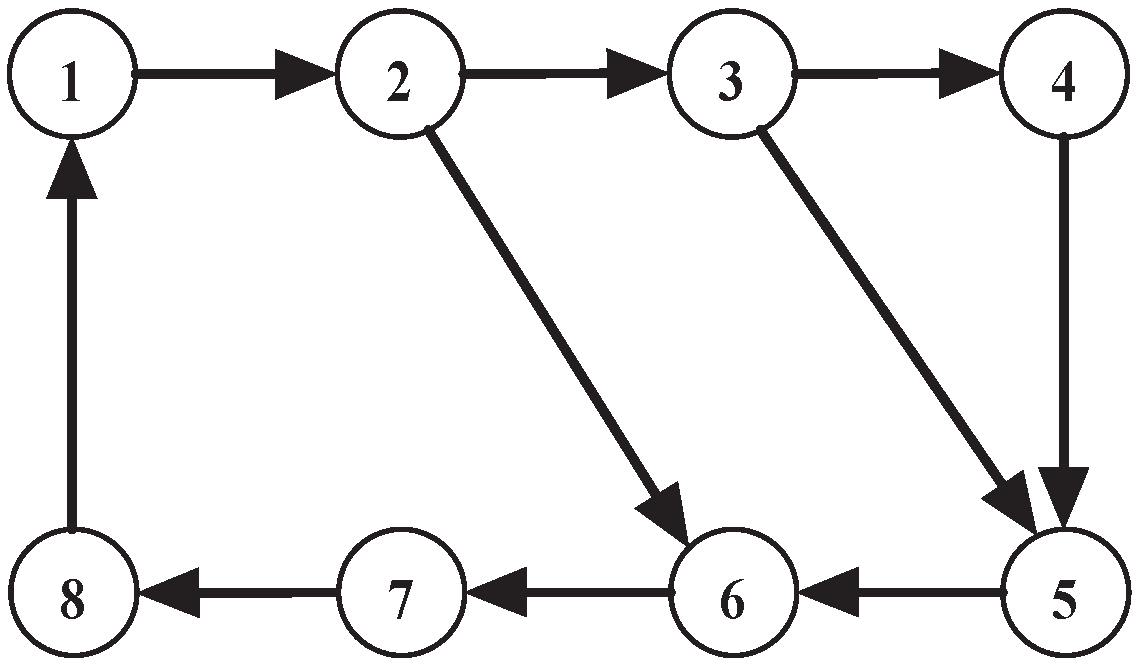
Moreover, it is assumed that the state of the moving target at the step t is contained in $K_{0,t}$, which is selected as $[-2,2]$ for all $t=1,2,3,4,5$. Additionally, the balanced communication graph necessarily involved in the distributed Algorithm 1 is depicted as in Figure 1. Accordingly, we selected the weighted matrix A as

$$\left(\begin{array}{cccccccc}1/3& 1/3& 0& 0& 0& 0& 0& 1/3\\ 1/3& 1/3& 1/3& 0& 0& 0& 0& 0\\ 0& 1/3& 1/3& 1/3& 0& 0& 0& 0\\ 0& 0& 1/3& 1/3& 1/3& 0& 0& 0\\ 0& 0& 0& 1/3& 1/3& 1/3& 0& 0\\ 0& 0& 0& 0& 1/3& 1/3& 1/3& 0\\ 0& 0& 0& 0& 0& 1/3& 1/3& 1/3\\ 1/3& 0& 0& 0& 0& 0& 1/3& 1/3\end{array}\right)$$

Moreover, the step-sizes are selected as $\alpha =0.01$, $\beta =0.2$, and $\eta =0.1$ in this simulation, respectively. Especially, in Figure 2, the transient behaviors of all $k_{i,t}\left(a\right)$ under Algorithm 1 are shown, which shows that all $k_{i,t}\left(a\right)$ under Algorithm 1 converge to the unique optimal solution $k^{*}={(-2,-1,0,1,2)}^T$.

Furthermore, with the same settings except that the unbalanced communication graph necessarily involved in the distributed algorithm (18) is depicted as in Figure 3 and the weighted matrix A is selected as

$$\left(\begin{array}{cccccccc}1/2& 0& 0& 0& 0& 0& 0& 1/2\\ 1/2& 1/2& 0& 0& 0& 0& 0& 0\\ 0& 1/2& 1/2& 0& 0& 0& 0& 0\\ 0& 0& 1/2& 1/2& 0& 0& 0& 0\\ 0& 0& 1/3& 1/3& 1/3& 0& 0& 0\\ 0& 1/3& 0& 0& 1/3& 1/3& 0& 0\\ 0& 0& 0& 0& 0& 1/2& 1/2& 0\\ 0& 0& 0& 0& 0& 0& 1/2& 1/2\end{array}\right),$$

the transient behaviors of all $k_{i,t}\left(a\right)$ under Algorithm 2 are shown in Figure 4, which shows that all $k_{i,t}\left(a\right)$ under Algorithm 2 converge to the unique optimal solution $k^{*}={(-2,-1,0,1,2)}^T$.

Moreover, in order to highlight the good performance at reducing the computational complexity compared to Algorithm 1 in [30], the simulations of Algorithm 1 in this paper and Algorithm 1 in [30] under the same settings are further made. Especially, we introduce the convergence index (CI) as

$$\mathrm{CI}={\displaystyle \frac{\parallel \frac{1}{N}{\displaystyle \sum _{i=1}^N}{k}_i\left(a\right)-k^{*}\parallel }{\parallel k^{*}\parallel }},$$

with $k_i\left(a\right)={(k_{i,1}\left(a\right),k_{i,2}\left(a\right),\cdots ,k_{i,N}\left(a\right))}^T$ and show the transient behaviors of CI under two Algorithms in Figure 5 for comparison. It can be seen from Figure 5 that two distinct Algorithms share a similar convergence rate. On the other hand, the operating time of GPU with different Algorithms is recoded during the simulations, which shows that for obtaining the similar convergence performance, $0.079$ s is required for Algorithm 1 in this paper, while $0.240$ s is needed for Algorithm 1 in [30].

Additionally, in order to explore how the momentum parameters affect the convergence rate, the simulations of Algorithm 1 with different momentum parameters are further made under the same other settings. Furthermore, the transient behaviors of CI under Algorithm 1 with different momentum parameters are shown in Figure 6 for comparison, which shows that the convergence rates in terms of the CI under Algorithm 1 with bigger momentum parameters are faster than that with smaller momentum parameters, and Algorithm 1 is nonconvergent when the momentum parameter is too big ($\eta \ge 1$).

Remark 2.

It is worth mentioning that although the definitions of the upper bound of the desired α, β, and η are given in Equations (12) and (13), it is still difficult to exactly give the explicit bounds of the desired α, β, and η since the global information L, μ, and ρ are necessarily involved in the definitions. On the other hand, it can also be noted from Equations (12) and (13) that the proposed Algorithms would be convergent when α, β, and η are sufficient small. Therefore, when carrying out the simulation for the proposed Algorithms, arbitrarily positive constants can be selected for the step-sizes first. Then, if the Algorithms with the selected step-sizes are nonconvergent, the smaller positive constants could be selected for the step-sizes until the Algorithms converge.

5. Conclusions

This paper has examined a constrained optimization problem within a closed convex set and designed a distributed algorithm incorporating momentum terms. Especially, the method of feasible direction and the method of estimating the left eigenvector have been employed to address the considered constraint and the unbalance, respectively. The algorithm’s linear convergence has been demonstrated with carefully chosen step-sizes, and the optimal ranges for these step-sizes are clearly defined. Compared to the existing algorithms designed in [30], the algorithm proposed in this paper has lower computational complexity. Simulation results have confirmed the algorithm’s effectiveness. Future research will explore the impact of time-varying graph sequences and more complex constraints. Furthermore, further research will also explore overcoming the limitation of the increased complexity with respect to operating the designed algorithms in large-scale drone networks, accompanied with the momentum terms. Additionally, further research will also explore the sensitivity analysis on step-size settings and momentum parameters.