UAV Autonomous Navigation Based on Deep Reinforcement Learning in Highly Dynamic and High-Density Environments

Abstract

Autonomous navigation of Unmanned Aerial Vehicles (UAVs) based on deep reinforcement learning (DRL) has made great progress. However, most studies assume relatively simple task scenarios and do not consider the impact of complex task scenarios on UAV flight performance. This paper proposes a DRL-based autonomous navigation algorithm for UAVs, which enables autonomous path planning for UAVs in high-density and highly dynamic environments. This algorithm proposes a state space representation method that contains position information and angle information by analyzing the impact of UAV position changes and angle changes on navigation performance in complex environments. In addition, a dynamic reward function is constructed based on a non-sparse reward function to balance the agent’s conservative behavior and exploratory behavior during the model training process. The results of multiple comparative experiments show that the proposed algorithm not only has the best autonomous navigation performance but also has the optimal flight efficiency in complex environments.

1. Introduction

Thanks to the rapid development of control algorithms and computing platforms, research on unmanned aerial vehicles has made a series of progress [1,2,3]. Due to their high efficiency, portability, and economy, Unmanned Aerial Vehicles (UAVs) are widely used in many fields, such as remote rescue [4,5], logistics delivery [6,7], environmental monitoring [8,9], and smart agriculture [10,11]. In most tasks performed by UAVs, their core role can be defined as the mission of flying between two points, and during this process the UAV can achieve automatic navigation and obstacle avoidance [12]. However, in real-life scenarios, high-density and highly dynamic working environments such as woods and pedestrians pose great challenges to the autonomous planning and navigation of UAVs, which requires the UAV to be able to effectively identify obstacles and respond in a timely manner [13,14]. Therefore, how to improve the autonomous flight performance of UAVs in complex environments has become a core issue for scholars and industry.

UAVs usually need to choose a reasonable path to the target point by evaluating perceived environmental information. In recent years, the development of deep reinforcement learning (DRL) has provided new solutions and ideas for autonomous UAV navigation, which learns and optimizes strategies through continuous trial and error [15,16,17,18]. Many classic DRL algorithms have been applied in the field of autonomous navigation of unmanned systems and deployed on real machines [19,20,21,22]. In actual research, Guo et al. [23] divided the autonomous navigation of a UAV into two subtasks, navigation and obstacle avoidance, and proposed a targeted distributed DRL framework. This method can achieve the navigation task of a UAV in a highly dynamic environment without prior knowledge. Liu et al. [24] proposed a hierarchical network architecture to improve the algorithm performance by introducing a temporal attention mechanism and verified it in real and simulated scenarios, but the test environment of the algorithm is relatively simple. In order to improve the interpretability of the model, Shao et al. [25] proposed a UAV collision avoidance scheme based on DRL, which improved the training speed of the model by introducing the idea of curriculum learning to achieve autonomous flight in a restricted closed environment. In response to the distribution differences between the simulated training environment and actual application environment of the DRL algorithm, reference [26] built a random environment generation platform to train the DRL model, and improved the stability of the model deployed on the real machine through dynamic training. Reference [27] uses light detection and ranging (LiDAR) measurement data as input and proposes an end-to-end autonomous navigation algorithm, which uses a fast stochastic gradient algorithm to solve the constraint model and realize autonomous navigation in complex 3D unknown environments. To improve the perception and tracking accuracy of UAVs, reference [28] combines the improved differential amplification method with the DRL algorithm. Compared with the traditional motion control method, the proposed DRL algorithm has stronger flexibility and better performance.

Although the effectiveness of DRL-based UAV autonomous navigation solutions has been proven by many studies, most algorithms are only tested in simulation environments with few obstacles and simple scenes, making it difficult to evaluate their application effects in complex environments with high-density and highly dynamic obstacles. In addition, there are several issues in current research that need further study: (1) Sparse rewards: The agent will only be rewarded when it reaches the goal point during model training. This typically makes it more difficult for the agent to effectively learn the correct behavior strategy during the exploration process, which causes the trained model to converge slowly or not at all [29,30]; (2) Exploration and utilization: The exploration of an agent means trying new behaviors to discover possible high-reward states, while utilization means selecting the current optimal behavior based on known information, which corresponds to the conservative and radical behavior of the UAV [31,32]; (3) State space: The choice of state space is crucial to the DRL model. Most agents only make decisions based on the information at the current moment, ignoring the dynamic changing trends of the agent (such as the translation and rotation of the UAV) [12,33].

Researchers have conducted targeted research on the above problems. Wang et al. [34] generated actions for the agent to interact with the environment by combining current strategies and prior strategies, and gradually improved the agent performance under sparse rewards by setting dynamic learning goals. However, higher complexity and constraints limit the further promotion of this algorithm. Wang et al. [33] built a two-stream Q network to process the temporal information and spatial information extracted from the UAV’s current moment state and the previous moment state, respectively. This algorithm provides a new idea for the selection of state space, but when using observation changes, it only considers the position changes caused by the translation of the UAV and ignores the angle changes caused by its rotation. Based on this, Zhang et al. [35] developed a two-stream Actor-Critic architecture by combining a two-stream network and TD3, and constructed a non-sparse reward function that can balance the exploration behavior and radical behavior of UAVs. This algorithm also ignores the angle information of the UAV, and essentially its reward function remains fixed during the entire training process.

Based on the above analysis, this paper proposes an improved UAV autonomous navigation algorithm based on SAC in view of the current status of UAV autonomous navigation based on DRL in complex environments. By analyzing the continuous maneuvering mechanism of UAVs in complex environments, a more reasonable state space is constructed; the comprehensive performance of the intelligent agent is improved by designing a dynamic reward function. Based on the proposed method, this paper realizes autonomous path planning of UAVs in high-density and highly dynamic environments. The main contributions are as follows:

(1)

The impact of UAV position changes and angle changes on navigation performance in complex scenarios was analyzed, and angle change information was introduced as input to the DRL model to expand ideas for research on LiDAR-based navigation algorithms;

(2)

A dynamic reward function is constructed based on a non-sparse reward function to balance the conservative behavior and exploratory behavior of the agent during the model training process, and improve the flight efficiency while improving the success rate of UAV navigation;

(3)

Flight simulation scenarios with high-density and highly dynamic obstacles were constructed, respectively, to verify the effectiveness and reliability of the proposed navigation algorithm.

The structure of subsequent chapters of this article is as follows: Section 2 introduces the theoretical background related to DRL. Section 3 formulates the DRL-based UAV navigation problem. Section 4 describes the algorithm proposed in this paper. Section 5 presents the experimental details and discusses the results. The last section summarizes this article and gives future work plans.

2. Background

2.1. Markov Decision Process (MDP)

MDP is a model decision framework based on Markov properties, consisting of five elements $\langle S,A,P,R,\gamma \rangle$, where $S$ represents the set of various states of the agent; $A$ represents the set of actions that the agent can choose; $P(s^{\prime }|s,a)$ describes the transition probability of the state; $R(s,a)$ is used to evaluate the reward obtained by the agent for taking a certain action; $\gamma \in [0,1]$ is used to measure the importance of future rewards.

In MDP, policy refers to the mapping from states and actions to action selection probabilities, which can be expressed as $\pi (a|s)=P(A_t=a|S_t=s)$. It is essentially the probability distribution of selecting action a when given state $s$. The policy $\pi (a|s)$ can be evaluated by the state value function $V^{\pi }(s)$ and the state-action value function $Q^{\pi }(s,a)$, where $V^{\pi }(s)$ is used to determine the future expected return that the agent will obtain starting from $s$ under the policy $\pi$, which is expressed as:

$$V^{\pi }(s)={\mathbb{E}}^{\pi }[G_t|S_t=s]$$

(1)

where $G_t$ represents the sum of all discount rewards from time $t$ onwards, which is expressed as:

$$G_t=R_t+\gamma R_{t+1}+{\gamma }^2{R}_{t+2}+\cdots ={\displaystyle \sum _{k=0}^{\infty }{\gamma }^k{R}_{t+k}}$$

(2)

Therefore, Equation (1) can be expressed as:

$$V^{\pi }(s)={\mathbb{E}}^{\pi }\left({\displaystyle \sum _{k=0}^{\infty }{\gamma }^k{R}_{t+k}|S_t=s}\right)$$

(3)

The state-action value function $Q^{\pi }(s,a)$ is used to indicate the future expected reward obtained after executing action $a$ in state $s$ when following policy π, which is expressed as:

$$Q^{\pi }(s,a)={\mathbb{E}}^{\pi }[G_t|S_t=s,A_t=a]$$

(4)

Similarly, Equation (4) can be further expressed as:

$$Q^{\pi }(s,a)={\mathbb{E}}^{\pi }\left({\displaystyle \sum _{k=0}^{\infty }{\gamma }^k{R}_{t+k}|S_t=s,A_t=a}\right)$$

(5)

The optimal value in the above equation represents the best performance of the agent in MDP problems.

2.2. SAC

The SAC algorithm combines the actor-critic method and the concept of entropy in RL. The core idea is to maximize the expected return while maintaining the randomness of the strategy, as follows:

$${\pi }^{\ast }=\arg \underset{\pi }{\max }{\displaystyle \sum _t{\mathbb{E}}_{(s_t,a_t)\sim {\rho }_{\pi }}\left[r\left(s_t,a_t\right)+\alpha \mathcal{H}\left(\pi \left(·|s_t\right)\right)\right]}$$

(6)

where $\alpha$ is the temperature parameter, which determines the relative importance of the entropy term relative to the reward, thus controlling the randomness of the optimal strategy.

In the maximum entropy RL framework, soft Q-value calculation iterates the mapping from state $S$ to action $A$ to reward $R$, and repeatedly corrects the Bellman operator. The Bellman equation and state value function can be further described as:

$$Q\left(s_t,a_t\right)\triangleq r\left(s_t,a_t\right)+\gamma {\mathbb{E}}_{s_{t+1}\sim \rho }\left[V\left(s_{t+1}\right)\right]$$

(7)

$$V\left(s_t\right)={\mathbb{E}}_{a_t\sim \pi }\left[Q\left(s_t,a_t\right)-\alpha \log \pi \left(a_t|s_t\right)\right]$$

(8)

Then, the strategy can be improved according to the following formula:

$${\pi }_{new}=\arg \underset{{\pi }^{\prime }}{\min }{D}_{KL}\left({\pi }^{\prime }\left(·|s_t\right),{\displaystyle \frac{\exp \left(\frac{1}{\alpha }{Q}^{{\pi }_{old}}\left(s_t,·\right)\right)}{Z^{{\pi }_{old}}\left(s_t,·\right)}}\right)$$

(9)

where $D_{KL}$ represents Kullback–Leibler (KL) divergence. The above formula can be used to improve the strategy in discrete space. In continuous spaces, it is necessary to approximate such iterations through parameterized functions and strategies. The detailed theory on this part can be found in [36].

3. Problem Formulation

3.1. Scenario Description

The tasks of UAVs are complex and diverse, especially in high-density and highly dynamic environments, which require excellent navigational performance. In order to facilitate modeling analysis, this article assumes that the UAV flies at a fixed altitude. As shown in Figure 1, the flight mission of the UAV can be represented as point-to-point flight, and the UAV needs to automatically identify and avoid obstacles during this process. Furthermore, we hope that the UAV will be able to finish the flight mission in the shortest possible path.

This paper generates UAV flight decisions based on the DRL algorithm to achieve autonomous flight and obstacle avoidance. The UAV senses environmental information based on LiDAR during flight. The current status information of the UAV is composed of environmental information, flight information, and target information. It is used as the input of the DRL model to obtain the next flight control command of the UAV, and the UAV will obtain new status information and rewards after executing the command. By constantly interacting with the environment, the UAV can continuously optimize its behavior and improve its ability to navigate and avoid obstacles autonomously.

3.2. Environment Perception Model

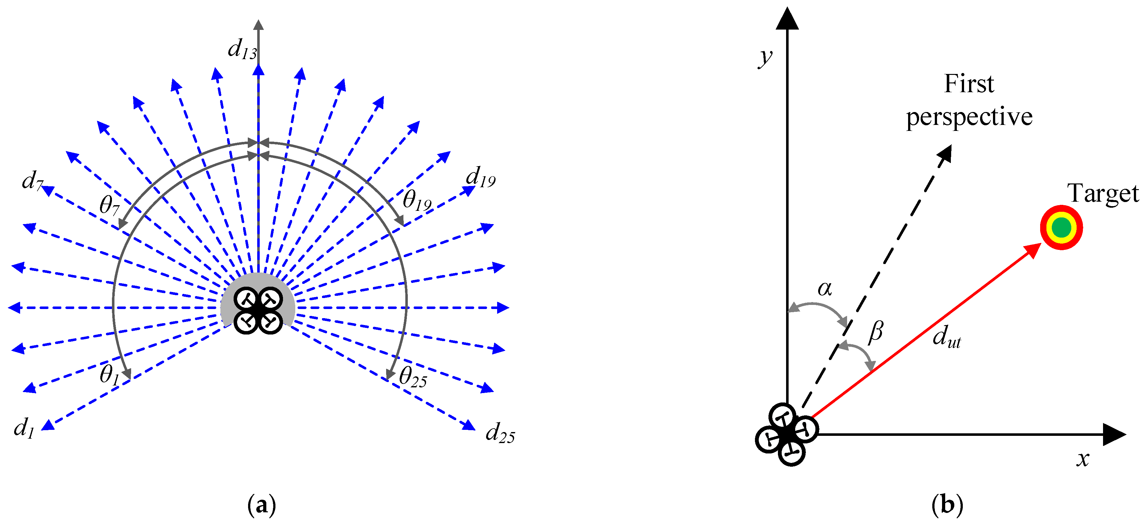
The airborne LiDAR model used in this article is shown in Figure 2a. The UAV measures the distance of surrounding obstacles through laser beams [37]. The field of view of LiDAR is $4\pi /3$ and the angular resolution is $\pi /18$. It can measure 25 sets of data in different directions at the same time. The measurement data at different times can be expressed as:

$$o_t=[d_1^t,\cdots d_i^t,\cdots ,d_{25}^t]$$

(10)

where $0.14\le d_i\le 3.5$ represents the measurement range of LiDAR; $\theta =[{\theta }_1,\cdots {\theta }_i,\cdots ,{\theta }_{25}]$ represents the angle corresponding to each laser beam. As mentioned in Section 3.1, in order to realize autonomous flight in complex environments, in addition to observation information, information about the UAV itself and target information are also needed. The UAV information available in this article includes linear velocity $v_{lin}$, yaw angular velocity $v_{yaw}$, linear acceleration $a_{lin}$, and yaw angular acceleration $a_{yaw}$. In addition, to ensure that the UAV moves toward the target point, we use relative coordinates to represent the positional relationship between the UAV and the target point. As shown in Figure 2b, $d_{ut}$ represents the relative distance between the UAV and the target point, $\alpha$ represents the yaw angle, and $\beta$ represents the angle between the UAV’s first perspective and the line connecting the UAV and the target point. Therefore, the state of the UAV can be described as:

$$s_u=\left[v_{lin},v_{yaw},a_{lin},a_{yaw},d_{ut},\beta \right]$$

(11)

As mentioned before, in order to obtain richer environmental information, references [33,35] constructed observation information containing static and dynamic changes in the environment based on LiDAR measurement data. The static information $o_t$ represents the observation data at the current moment, and the dynamic information $\Delta o_t$ can be expressed as:

$$\begin{array}{cc}\hfill \Delta o_t& =o_t-o_{t-1}\hfill \\ & =[d_1^t-d_1^{t-1},\cdots ,d_i^t-d_i^{t-1},\cdots ,d_{25}^t-d_{25}^{t-1}]\hfill \end{array}$$

(12)

Dynamic information can provide the movement trend of the UAV relative to obstacles and help optimize the flight decision of the UAV.

3.3. DRL-Based Navigation Model

The UAV autonomous navigation model based on DRL mainly involves the UAV’s state space, action space, reward function, and network structure and other elements.

State space s is the basis for the DRL model to make UAV flight decisions, and it is crucial for UAV navigation. As mentioned in Section 3.2, the state space mainly includes environmental information and the UAV’s own information, which can be expressed as:

$$\begin{array}{cc}\hfill s_t& =\left[o_t,s_u^t\right]\hfill \\ & =\left[d_1^t,\cdots d_i^t,\cdots ,d_{25}^t,v_{lin}^t,v_{yaw}^t,a_{lin}^t,a_{yaw}^t,d_{ut}^t,{\beta }^t\right]\hfill \end{array}$$

(13)

According to Equation (13), the dimension of the UAV’s state space s is 31. In addition, in order to accelerate the convergence of the method, the state space s will be normalized before inputting to the model.

The action space a is made up of its linear velocity $v_{lin}$ and yaw angular velocity $v_{yaw}$, since it flies at a predetermined height. In addition, to ensure the stability of the UAV, the actual flight speed of the UAV will be limited as follows:

$$v_{lin}\in [0,0.5],v_{yaw}\in [-1,1]$$

(14)

After obtaining the action command, the UAV updates its attitude and position by adjusting the motor speed to execute the command.

The main function of the reward function is to convey the goal to the agent, that is, to maximize the expected probability value of the cumulative sum of reward signals received by the agent. The agent will receive a corresponding reward after performing an action, so the design of the reward function directly determines the performance evaluation of the agent on a specific action, which in turn affects the performance and convergence speed of the DRL method. The reward function described in this article is as follows [26]:

$$\begin{array}{cc}\hfill R& =r_{dis}+r_{arr}+r_{cra}\hfill \\ & +r_{laser}+r_{step}+r_{lin}+r_{yaw}\hfill \end{array}$$

(15)

where $r_{dis}$ represents the distance reward, $r_{arr}$ represents the reward for reaching the target, $r_{cra}$ represents the reward for hitting the obstacle, $r_{laser}$ represents the free space reward, $r_{step}$ represents the step reward, $r_{lin}$ and $r_{yaw}$ represent the linear acceleration and yaw angular acceleration rewards, respectively, and their specific expressions are as follows:

$$r_{dis}={\epsilon }_1\left(d_{ut}^t-d_{ut}^{t-1}\right)$$

(16)

$$r_{arr}=\{\begin{array}{c}100, \mathrm{if} d_{ut}\le 0.4\hfill \\ 0,\mathrm{else}\hfill \end{array}$$

(17)

$$r_{cra}={\epsilon }_2\{\begin{array}{c}-10, 0.5\le \min (o)<0.7\hfill \\ -25, 0.25\le \min (o)<0.5\hfill \\ -100, \min (o)<0.25\hfill \end{array}$$

(18)

$$r_{laser}=-{{\displaystyle {\sum }_i\left(1-d_i/\max \left(o\right)\right)}}^4$$

(19)

$$r_{step}=-{\epsilon }_3\ast N_{step}$$

(20)

$$r_{lin}=-{\epsilon }_4\ast \left|a_{lin}\right|$$

(21)

$$r_{yaw}=-{\epsilon }_5\ast \left|a_{yaw}\right|$$

(22)

where $N_{step}$ represents the number of steps performed by the drone, and ${\epsilon }_1$ to ${\epsilon }_5$ usually represent fixed constants.

4. Proposed Approach

4.1. State Space Representation Method

As mentioned in Section 3, the state space is crucial to the performance of DRL models. In autonomous UAV navigation tasks based on LiDAR, most studies directly use the LiDAR-measured data shown in Equation (10) as observation information. Reference [33] proves that the flight performance of the UAV is further improved after adding dynamic information as observation information, but the impact of changes in the angle of the UAV is not considered.

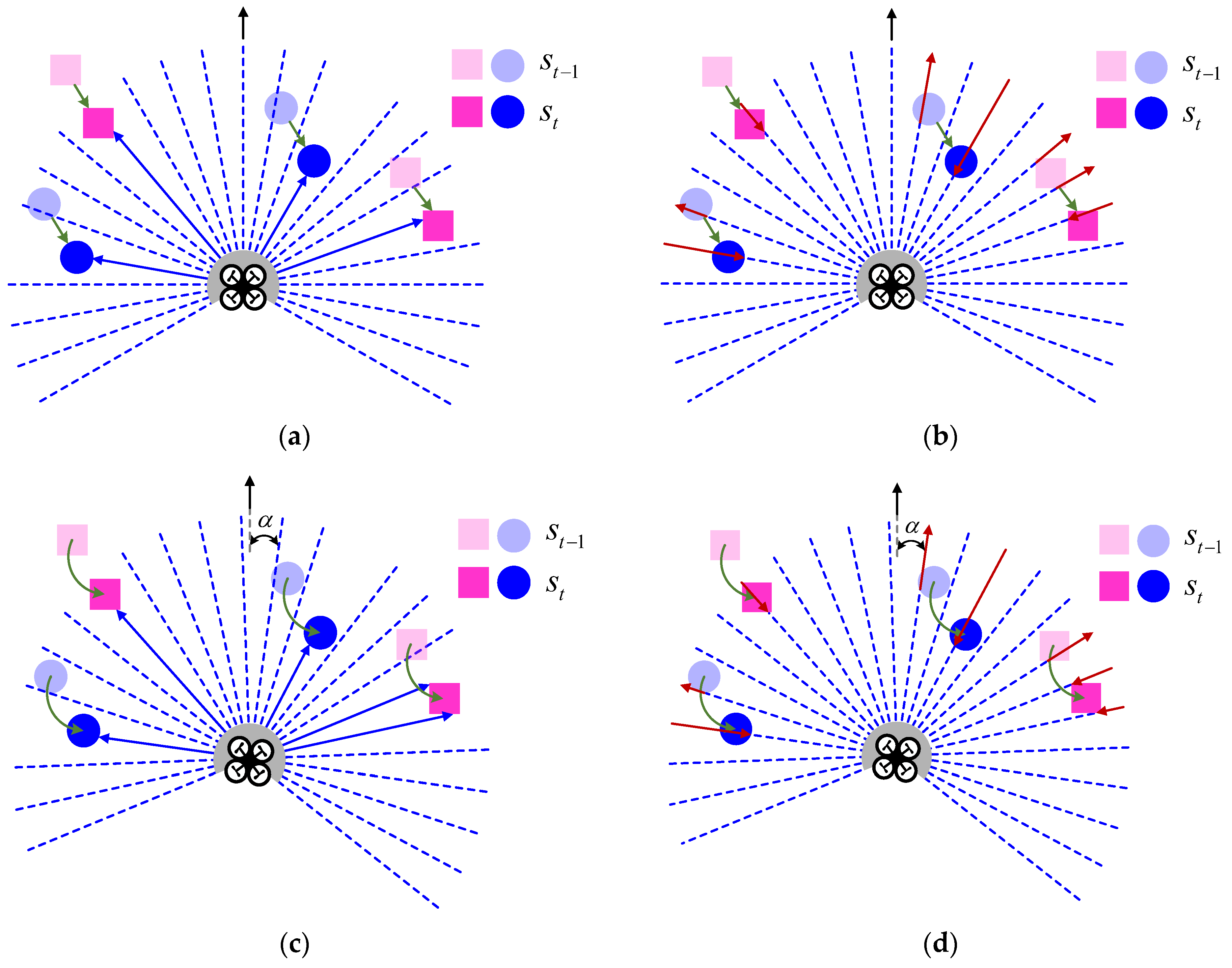
As shown in Figure 3a,b, LiDAR can obtain a set of measurement data at time t, and the UAV can estimate the distance and distribution of surrounding obstacles based on $o_t$. Compared with time t-1, the position of the UAV relative to the obstacle has changed, and the change value $\Delta o_t$ of the measurement data at adjacent moments can provide the movement trend of the UAV relative to the obstacle. As shown in Figure 3c,d, the attitude changes of the UAV during actual flight include not only changes in position but also changes in flight angle.

Based on the above analysis, this paper proposes a state space representation method that considers angle change information. First, add the angle information corresponding to the laser beam when obtaining the LiDAR measurement data $o_t$, as shown below:

$$o_t=[d_1^t,{\theta }_1,\cdots ,d_i^t,{\theta }_i,\cdots ,d_{25}^t,{\theta }_{25},{\alpha }^t]$$

(23)

Furthermore, according to Equation (12), the dynamic information $\Delta o_t$ at adjacent moments after adding angle information can be expressed as:

$$\begin{array}{cc}\hfill \Delta o_t& =o_t-o_{t-1}\hfill \\ & =[d_1^t-d_1^{t-1},0,\cdots ,d_i^t-d_i^{t-1},0,\cdots ,d_{25}^t-d_{25}^{t-1},0,{\alpha }^t-{\alpha }^{t-1}]\hfill \end{array}$$

(24)

Since the corresponding angle ${\theta }_i$ of the laser beam is fixed, Equation (24) can be further simplified as follows:

$$\begin{array}{cc}\hfill \Delta o_t& =[d_1^t-d_1^{t-1},\cdots ,d_i^t-d_i^{t-1},\cdots ,d_{25}^t-d_{25}^{t-1},{\alpha }^t-{\alpha }^{t-1}]\hfill \\ & =[\Delta d_1^t,\cdots ,\Delta d_i^t,\cdots ,\Delta d_{25}^t,\Delta {\alpha }^t]\hfill \end{array}$$

(25)

where $\Delta {\alpha }^t$ represents the change value of yaw angle. As shown in Figure 4, when the obstacles in the flight environment are stationary or the density is relatively sparse, the impact of changes in flight angle is not obvious. However, when the UAV flies in a highly dynamic or high-density complex environment, the angle change of the UAV can be expressed as:

$$\Delta {\alpha }^t=v_{yaw}^{t-1}·\Delta t+0.5a_{yaw}^{t-1}·\Delta t^2$$

(26)

The above formula shows that when the time interval is $\Delta t$, the yaw angle of the UAV changes, and the impact of this change on the UAV’s flight decision-making in a complex environment cannot be ignored.

Based on the above analysis, the DRL model state space determined in this article is as follows:

$$s_t=\left[o_t,\Delta o_t,s_u^t\right]$$

(27)

According to the Equations (14) and (27), the dimension of the state space in this paper is 83, the action space dimension is 2, and the network architecture adopted by the algorithm is shown in Figure 5.

4.2. Dynamic Reward Function

During the training process of the agent, how to balance the conservative and radical behavior of the agent is the focus that needs to be paid attention to. For UAVs, conservative means that the UAV is as safe as possible to avoid suffering larger penalties, while radical means that the UAV is more inclined to receive larger rewards and perform risky behaviors. If the agent obtains a larger reward after executing action a, it means that the action is more conducive to achieving the goal. Therefore, when the strategy is updated, the agent is more likely to subsequently choose to perform this action.

The non-sparse reward function designed in the current study usually remains unchanged during the training process of the agent. In fact, we hope that in the early stages of model training, the agent can be more radical to explore more possibilities. With the training of the model, the agent gradually tends to be conservative after it has the basic ability to complete tasks, thereby encouraging the agent to improve its own performance on the basis of ensuring its own safety.

Based on the above analysis, this paper proposes a dynamically changing reward function. By adjusting the distance reward $r_{dis}$, step reward $r_{step}$, and collision reward $r_{cra}$, the agent is given gradually changing guidance at different stages of training to improve its overall performance. They can be expressed as:

$$\begin{array}{l}{r}_{dis}={\epsilon }_1\left(d_{ut}^t-d_{ut}^{t-1}\right)\\ s.t.{\epsilon }_1=\{\begin{array}{c}{r}_1+{\displaystyle \frac{E_{step}}{2}},E_{step}\le 0.5E_{\max }\hfill \\ r_2,E_{step}>0.5E_{\max }\hfill \end{array}\end{array}$$

(28)

$$\begin{array}{l}{r}_{cra}={\epsilon }_2\{\begin{array}{c}-10, 0.5\le \min (o)<0.7\hfill \\ -25, 0.25\le \min (o)<0.5\hfill \\ -100, \min (o)<0.25\hfill \end{array}\\ s.t.{\epsilon }_2=\{\begin{array}{c}0.5+{\displaystyle \frac{E_{step}}{E_{\max }}},E_{step}\le 0.5E_{\max }\hfill \\ 1,E_{step}>0.5E_{\max }\hfill \end{array}\end{array}$$

(29)

$$\begin{array}{l}{r}_{step}=-{\epsilon }_3\ast N_{step}\\ s.t.{\epsilon }_3=\{\begin{array}{c}1-{\displaystyle \frac{E_{step}}{E_{\max }}},E_{step}\le 0.5E_{\max }\hfill \\ 0.5,E_{step}>0.5E_{\max }\hfill \end{array}\end{array}$$

(30)

where $E_{step}$ represents the current number of training rounds; $E_{\max }$ represents the set maximum number of rounds; $r_1$ and $r_2$ are constants set according to the task.

By changing the parameters ${\epsilon }_1$, ${\epsilon }_2$, and ${\epsilon }_3$, the reward function is dynamically adjusted in different training stages. In the initial stage of training, the agent is encouraged to explore the environment by giving smaller distance rewards and collision penalties. As training proceeds, the distance reward and collision penalty are increased while the step penalty is decreased to encourage the agent to stay away from obstacles.

5. Experiment and Discussion

5.1. Experimental Settings

In order to verify the algorithm proposed in this article, simulation scenarios of high-density and highly dynamic obstacles were built based on gazebo. The training scene for algorithms is shown in Figure 6, where there are 75 cylindrical obstacles with a radius of 0.15 and 75 cuboid obstacles with a side length of 0.2 in a 20 × 20 rectangular field. In each episode training, the coordinates of all obstacles are randomly generated and the target point is randomly selected among [0, 7], [0, −7], [7, 0], and [−7, 0]. The flight mission of the UAV is defined as flying from the origin to the destination within a specified number of steps, and the criteria for the end of each episode include: (1) the UAV successfully reaches the destination; (2) the UAV collides with an obstacle; (3) the UAV neither reaches the target nor collides within the maximum number of steps.

In order to verify the advantages of the method proposed in this article, DDPG, TD3, and SAC are used for comparison. All three algorithms use fixed reward functions and traditional state space expressions. In addition, in order to objectively evaluate the performance of the algorithm, we choose the following five quantitative indicators to measure the completion of the task.

(1)

Success rate $R_s$: the proportion of the number of times the UAV completes the navigation task to the total number of trials;

(2)

Collision rate $R_c$: the proportion of the number of times the UAV encountered obstacles to the total number of trials;

(3)

Loss rate $R_l$: the proportion of the number of times the UAV neither reaches the target point nor collides within the specified number of steps to the total number of trials;

(4)

Average flight distance $L_{dis}$: the average distance flown by the UAV when it successfully completes its mission;

(5)

Average number of flight steps $N_{step}$: the average number of steps required for the UAV to successfully complete the mission.

Among the above indicators, the larger $R_s$ is, the better the autonomous navigation performance of the UAV is. The smaller $L_{dis}$ and  are, the higher the flight efficiency of the UAV is.

5.2. Training Results

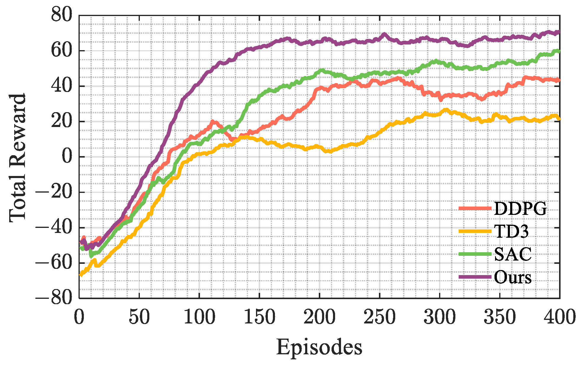
The proposed method and the three comparison algorithms are deployed on the hardware platform of Intel Core i5-11400F CPU @2.6 GHz × 12 and NVIDIA GTX 1650. For objective comparison, the training settings of the four algorithms are consistent, with the replay buffer size of 10,000, the network discount rate of 0.99, the batch size of 512, and the same network structure. In addition, the parameters of the reward function in Section 4.2 are set to $r_1=200$, $r_2=300$, and $E_{\max }=400$, respectively. The results of the cumulative rewards of different algorithms changing with the number of training episodes are shown in Figure 7. All data in the figure have been smoothed.

According to Figure 7, the proposed algorithm has faster convergence speed and higher reward than the other three algorithms, among which our algorithm starts to converge around the 150th episode, SAC and DDPG start to converge around the 200th episode, while TD3 starts to converge around the 300th episode and has the lowest reward. Therefore, the training results show that the proposed algorithm has better convergence.

5.3. Experiment I: High-Density Scene Verification

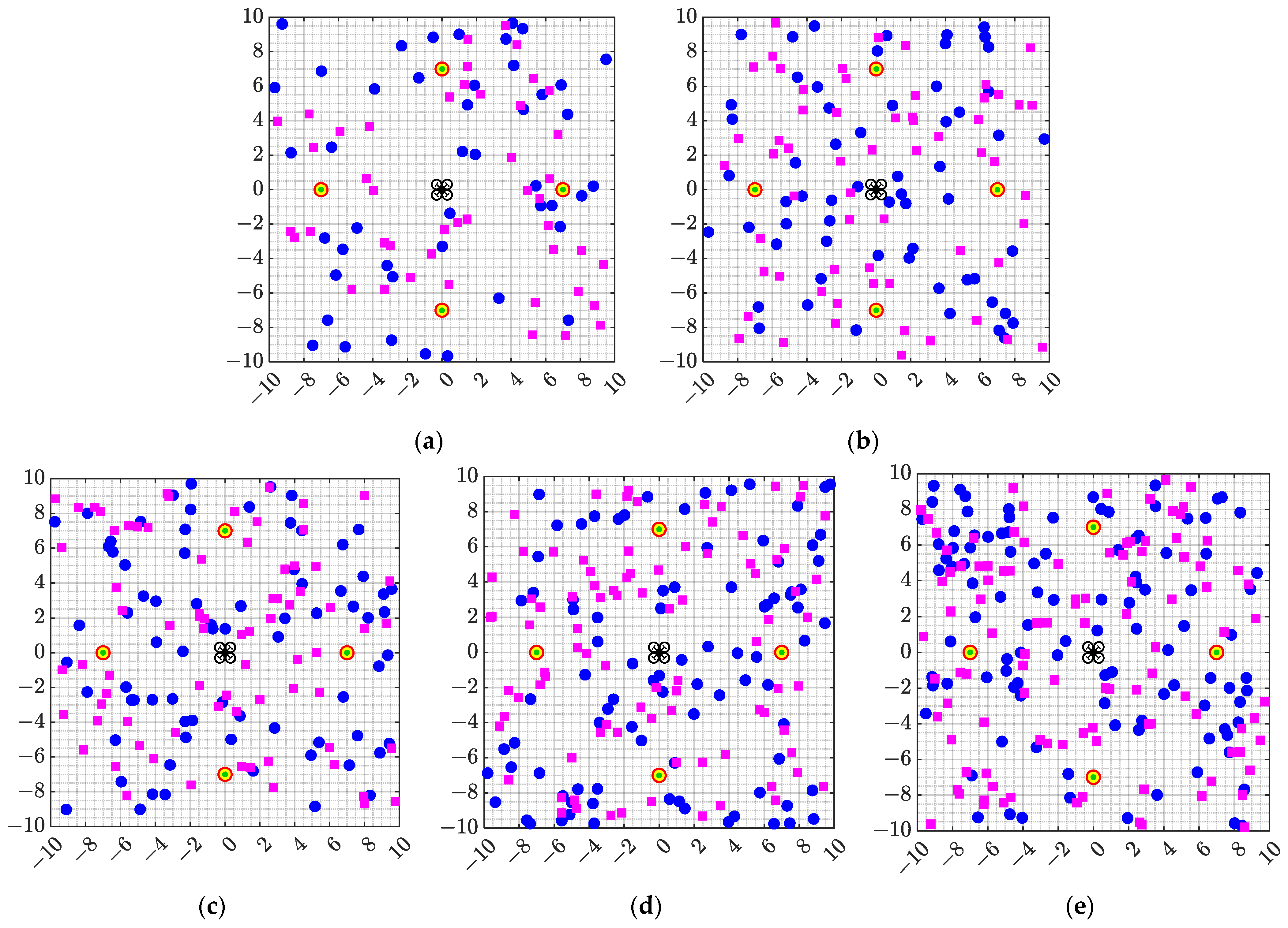
In order to verify the effect of the proposed algorithm, the DRL model trained in Section 5.2 was tested in simulation scenarios with different numbers of obstacles. The test scene is shown in Figure 8, where $N_{obs}$ represents the number of obstacles, and ρ represents the obstacle density, which is used to measure the density of obstacles present per unit area.

The UAV based on the four algorithms performed 100 navigation missions in five scenarios with different obstacle densities. Similar to the training process, the location of the obstacles was re-randomly generated and the target point was re-selected after each flight mission.

The navigation success rate $R_s$, collision rate $R_c$, and loss rate $R_l$ of the four algorithms under different obstacle densities are shown in

Table 1. Experimental results under different density scenarios.

Algorithm	Scene 1			Scene 2			Scene 3			Scene 4			Scene 5
	Rs	Rc	Rl	Rs	Rc	Rl	Rs	Rc	Rl	Rs	Rc	Rl	Rs	Rc	Rl
DDPG	87	12	1	81	18	1	65	34	1	64	36	0	59	41	0
TD3	73	27	0	59	41	0	49	51	0	32	68	0	25	75	0
SAC	94	6	0	93	7	0	87	13	0	73	27	0	65	35	0
Ours	97	3	0	96	4	0	93	7	0	86	14	0	79	21	0

. As can be seen from the table, the proposed algorithm achieved the highest navigation success rate and the lowest collision rate in all five scenarios, and the navigation performance of the SAC algorithm is better than DDPG and TD3. Due to the high density of obstacles in the experimental scene, only DDPG experienced flight loss. Comparing the experimental results of scene 1 and scene 5, it can be seen that with the substantial increase in obstacle density, the success rate of our algorithm is only reduced by 18%, while the success rates of the other three algorithms are reduced by 28%, 48%, and 29%, which further demonstrates the stability of our algorithm.

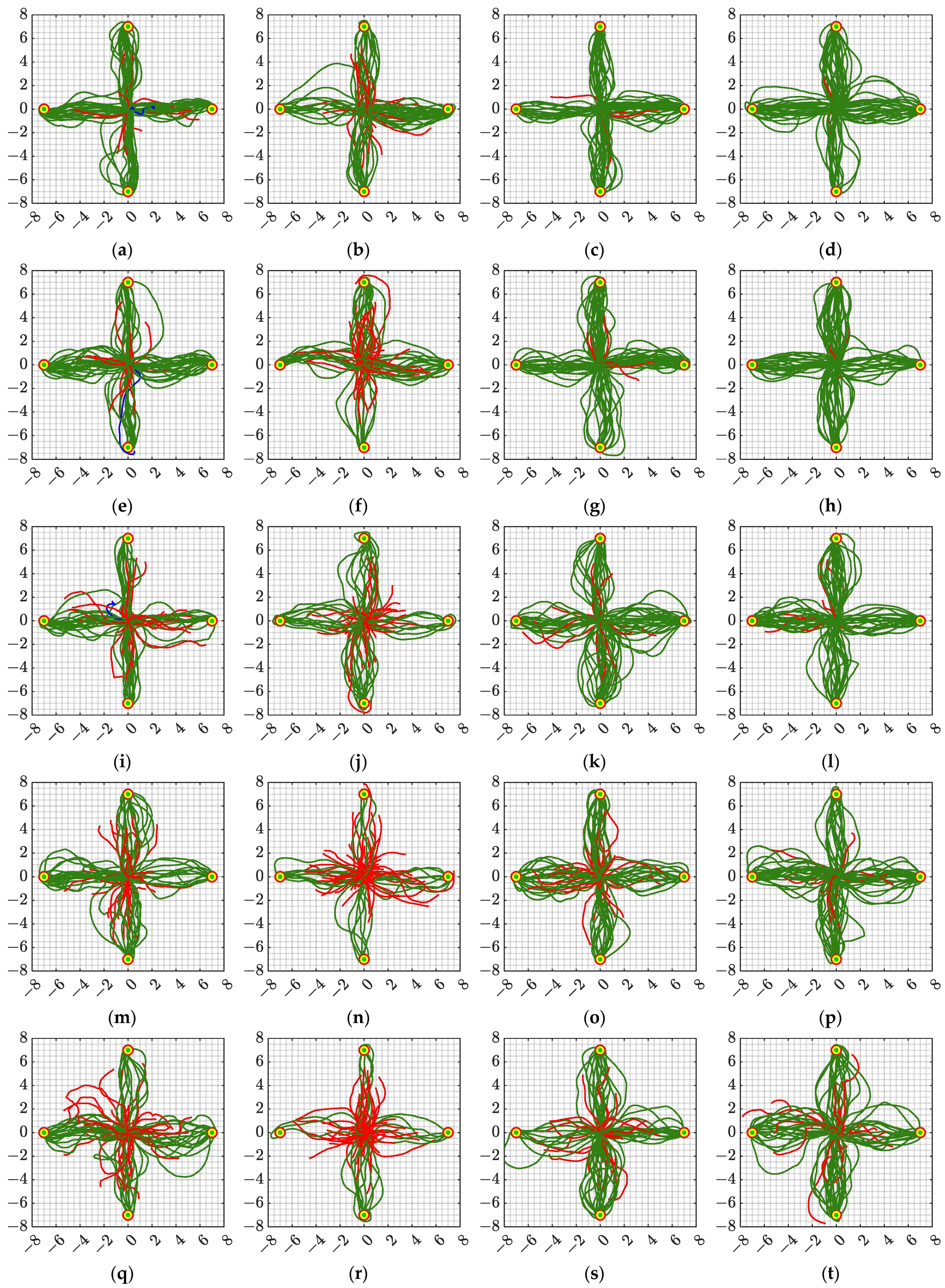
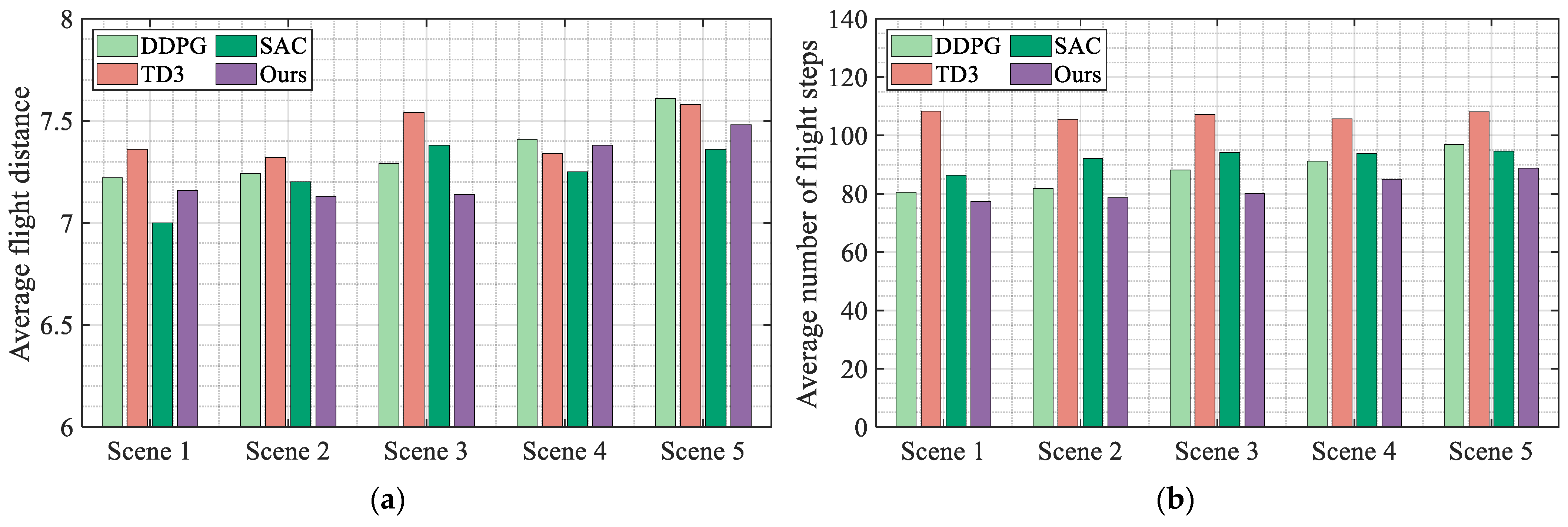
The flight trajectories of the UAV in all tests are shown in Figure 9. As can be seen from the figure, the algorithm proposed in this article has the most successful flight trajectories in all scenarios. In addition, as the density of obstacles increases, the flight path of the UAV becomes more complex. Based on the flight trajectory data, the average flight distance and average number of flight steps for all experiments were calculated, as shown in Figure 10.

According to Figure 10a, the proposed algorithm has the shortest average flight distance in scenarios 2 and 3, and has an average flight distance only larger than SAC in scenarios 1 and 5. According to Figure 10b, the proposed algorithm requires the minimum average number of flight steps in all five scenarios. Therefore, based on the above analysis, it can be seen that compared with the other three classic algorithms, the algorithm proposed in this article not only has the highest navigation success rate and stability but also has the optimal flight efficiency in high-density flight environments.

5.4. Experiment II: Highly Dynamic Scene Verification

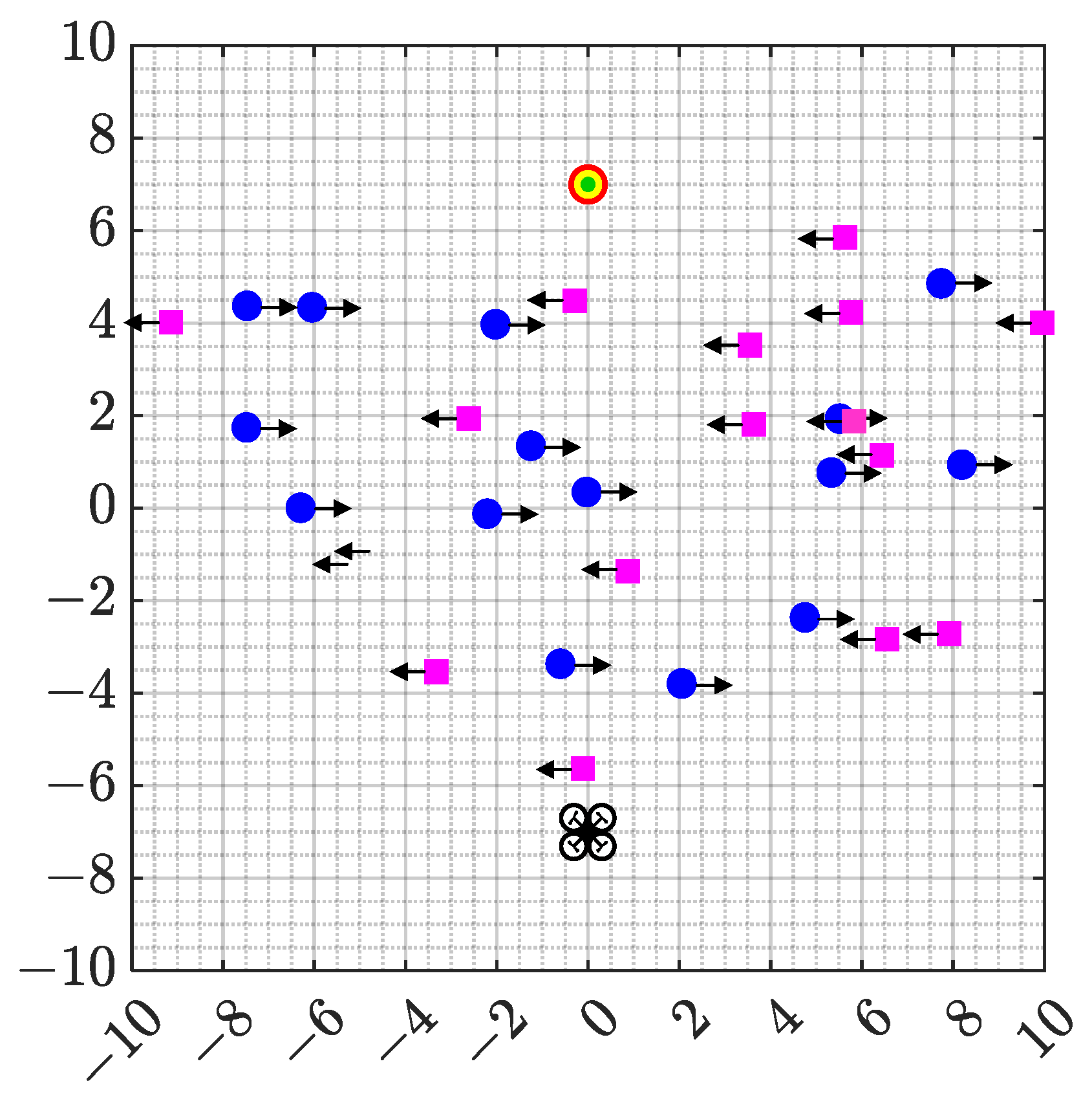
To further verify the performance of the trained algorithm, a dynamic test scenario is constructed as shown in Figure 11. The starting and target points are represented in the figure as [0, −7] and [0, 7], respectively. The UAV’s flight mission is defined as autonomous flight from the starting point to the target point. During each test, 30 obstacles are randomly generated in the test area. The movement direction of the obstacles is marked by the arrow in the figure. After reaching the edge of the field, the obstacles will continue to move in the opposite direction until the end of this test. The moving speeds of the obstacles are set at 0.01 m/s, 0.05 m/s, 0.1 m/s, 0.15 m/s, and 0.2 m/s, respectively. Each set of experiments is performed 100 times, and the position of the obstacle will be regenerated after each test.

The experimental results of all algorithms in five dynamic scenes are presented in

Table 2. Experimental results under different dynamic scenarios.

Algorithm	Scene 1			Scene 2			Scene 3			Scene 4			Scene 5
	Rs	Rc	Rl	Rs	Rc	Rl	Rs	Rc	Rl	Rs	Rc	Rl	Rs	Rc	Rl
DDPG	70	16	14	63	16	21	52	28	20	48	40	12	34	60	6
TD3	61	38	1	61	38	1	53	46	1	40	60	0	24	72	4
SAC	80	4	16	79	7	14	68	20	12	51	44	5	29	63	8
Ours	100	0	0	94	6	0	81	19	0	63	37	0	42	58	0

. It can be seen from the table that the proposed algorithm achieved the highest navigation success rate and the lowest collision rate in the experiments under different moving speeds of obstacles, and no flight loss occurred, which shows the effectiveness of the proposed algorithm in highly dynamic scenarios. For comparison, the other three algorithms all experienced flight loss, among which SAC and DDPG had higher loss rates. It should be noted that as the speed of obstacle movement increases, the difficulty for the UAV to avoid obstacles increases sharply, resulting in a significant reduction in the success rate of all algorithms.

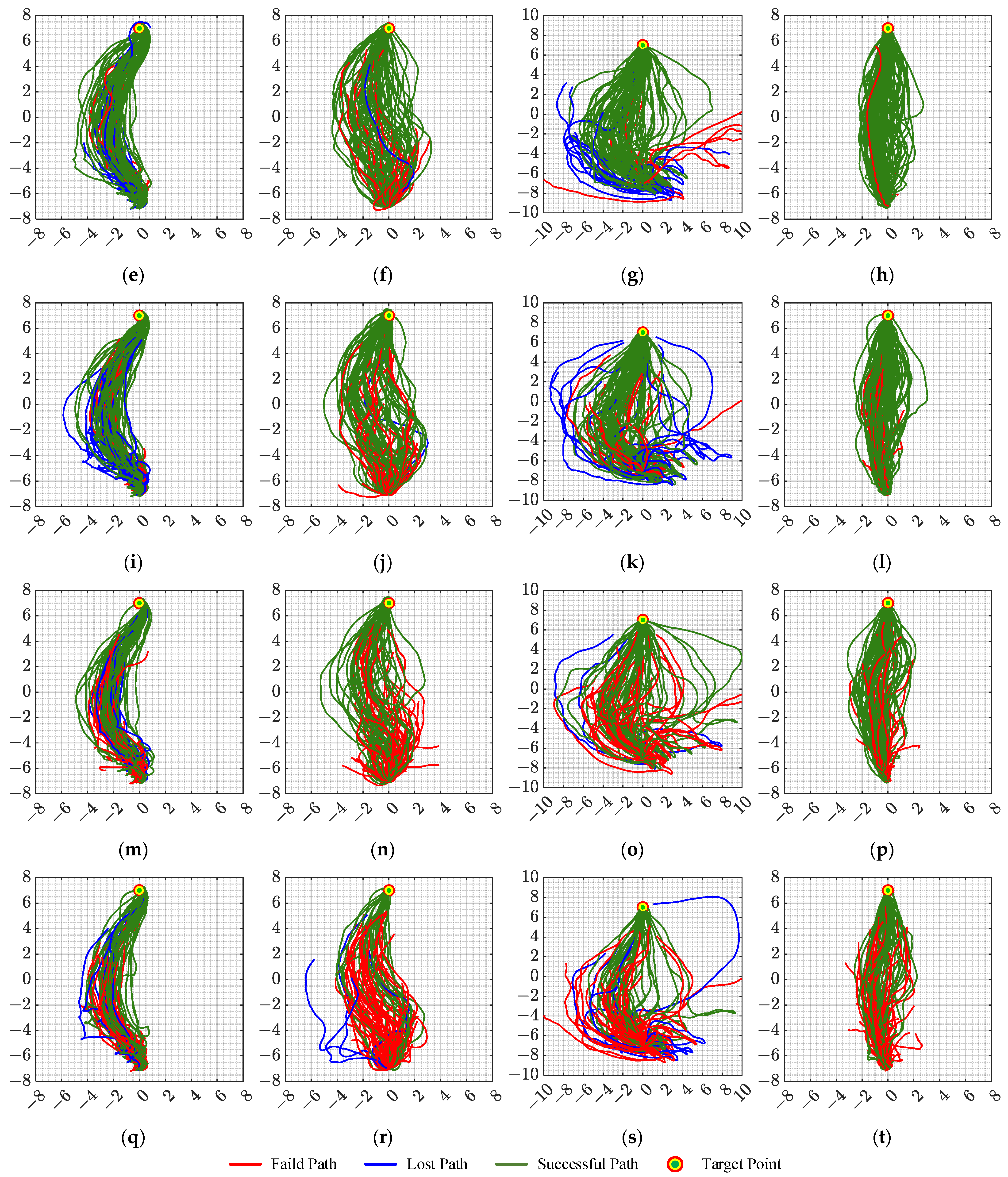
The flight trajectory of the UAV in the highly dynamic test is shown in Figure 12. It can be seen from the flight trajectory in the figure that the algorithm proposed in this article can fly from the starting point to the target point more directly, while several other algorithms have more messy flight trajectories, which shows that the proposed algorithm can not only adapt to high-density flight environments, but also apply to highly dynamic scenarios that have not appeared in the training phase. Based on the flight trajectory of the UAV, the average flight distance $L_{dis}$, and the average number of flight steps $N_{step}$ of the UAV in the dynamic scenario are calculated, as shown in Figure 13.

As can be seen from Figure 13, the proposed algorithm has the shortest average flight distance and the least average number of flight steps in all five dynamic flight scenarios. Corresponding to the flight trajectory in Figure 12, although SAC has a higher navigation success rate than TD3 and DDPG, its required flight distance is much higher than other algorithms. The TD3 algorithm has a lower average flight distance but the largest number of flight steps, which shows that the algorithm is more “cautious” in dynamic scenes. Figure 13 shows that the proposed algorithm not only has a high navigation success rate but also has the highest navigation efficiency when facing a highly dynamic flight environment, enabling the UAV to achieve autonomous navigation quickly and accurately.

5.5. Experiment III: Verify the Validity of the Reward

Experiments on UAVs in high-density and highly dynamic scenarios verified the effectiveness and reliability of the proposed algorithm. Based on the analysis in Section 4.2, we constructed “radical” and “conservative” reward function models by setting different step rewards, collision rewards, and distance rewards in order to further compare and illustrate the effect of the dynamic reward function designed in this article. The specific description is as follows:

Model 1: Based on Formulas (28)–(30), set ${\epsilon }_1=\left(r_1+r_2\right)/2$, ${\epsilon }_2=1$, ${\epsilon }_3=0.5$, respectively. By giving the agent a smaller step penalty and a larger collision penalty, the agent tends to choose a conservative behavior away from obstacles.

Model 2: Based on Formulas (28)–(30), set ${\epsilon }_1=\left(r_1+r_2\right)/2$, ${\epsilon }_2=0.5$, ${\epsilon }_3=1$, respectively. By giving the agent a larger step penalty and a smaller collision penalty, the agent is inclined to choose radical behavior to explore the environment.

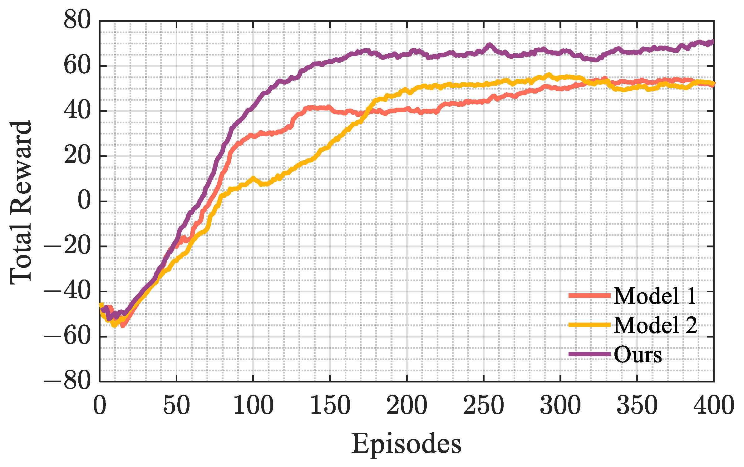
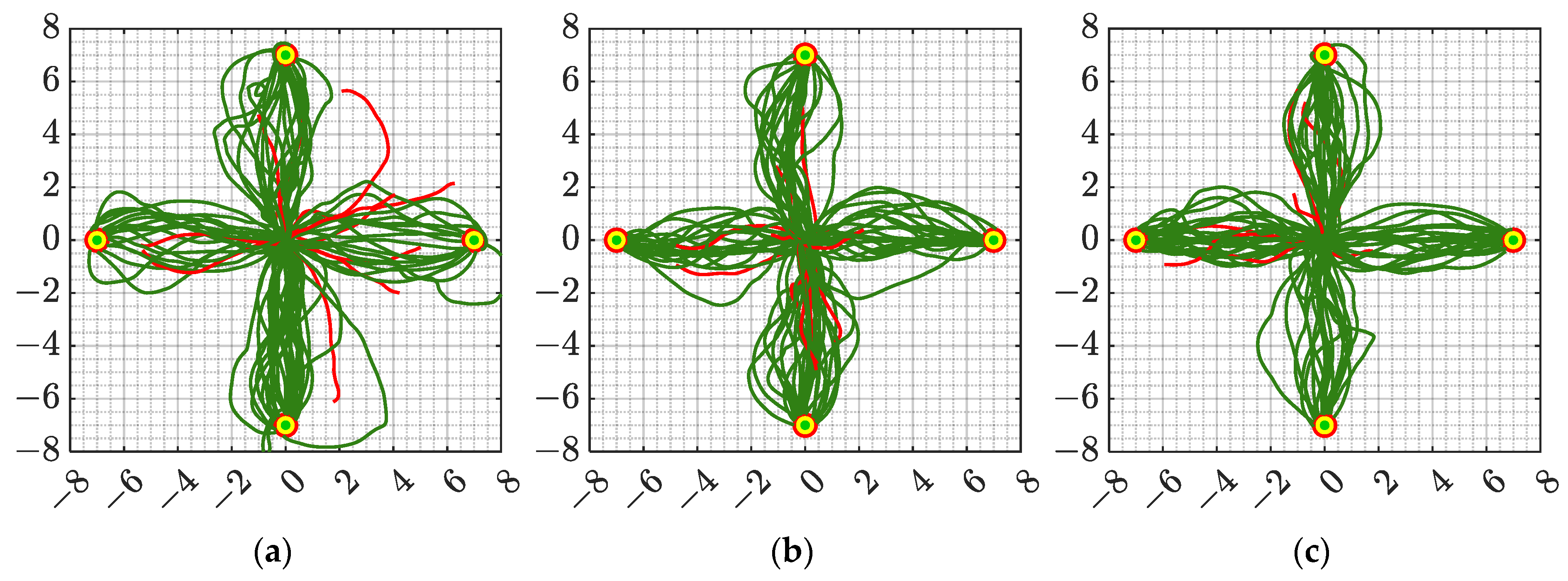
Models with different reward functions were trained in the simulation scenario shown in Figure 6, and the reward convergence curve obtained is shown in Figure 14.

It can be seen from the figure that compared with the other two models, the model proposed in this article has the fastest convergence speed and optimal reward. In addition, since model 1 has a more “conservative” reward function, it converges faster than model 2 in the early stage of training, and model 2 explores a better strategy after a period of training, so it converges faster than model 1.

In order to verify the performance of the two trained models, the high-density simulation environment shown in Figure 8c–e is used for testing. The test results are shown in

Table 3. Experimental results of models with different reward functions in high-density scenarios.

Algorithm	Scene 3			Scene 4			Scene 5
	Rs	Rc	Rl	Rs	Rc	Rl	Rs	Rc	Rl
Model 1	88	12	0	81	19	0	77	23	0
Model 2	88	12	0	77	23	0	75	25	0
Ours	93	7	0	86	14	0	79	21	0

. As can be seen from the table, comparing the two algorithms with fixed reward functions, the proposed algorithm has the highest navigation success rate in all scenarios, and the navigation success rate of model 1 is slightly higher than that of model 2.

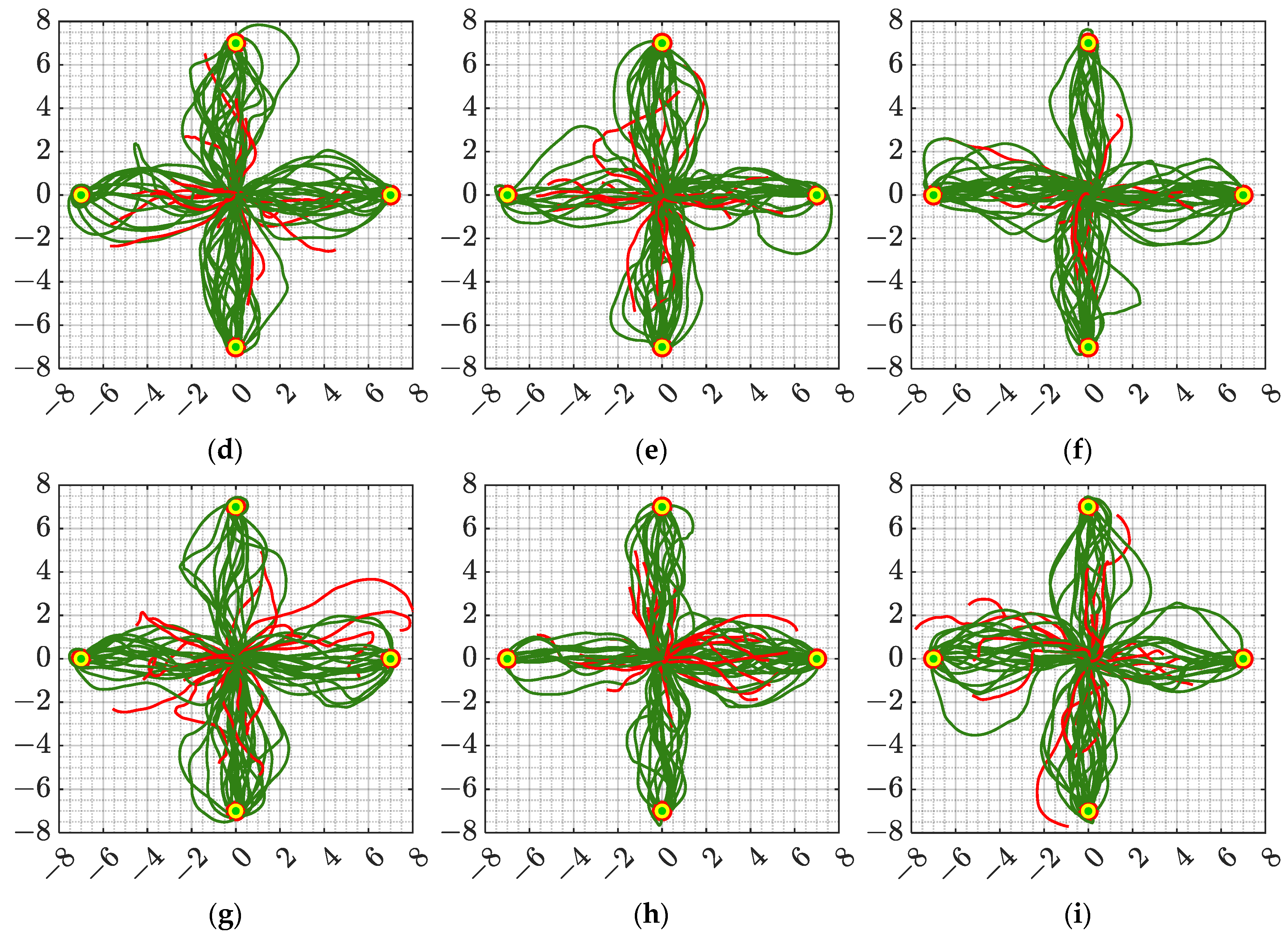
The flight trajectory of the UAV in the test is drawn as shown in Figure 15, and the average flight distance and average number of flight steps calculated based on the flight trajectory are shown in Figure 16. Combining all the experimental results in the figure, it can be seen that the proposed algorithm has the optimal flight efficiency.

Model 1 and model 2 were verified in highly dynamic scenarios with obstacle movement speeds of 0.1 m/s, 0.15 m/s, and 0.2 m/s, respectively. The obtained test results and UAV flight trajectories are shown in

Table 4. Experimental results of models with different reward functions in highly dynamic scenarios.

Algorithm	Scene 3			Scene 4			Scene 5
	Rs	Rc	Rl	Rs	Rc	Rl	Rs	Rc	Rl
Model 1	79	21	0	52	48	0	37	63	0
Model 2	62	37	1	36	64	0	26	74	0
Ours	81	19	0	63	37	0	42	58	0

and Figure 17 and Figure 18.

As can be seen from Table 4, the proposed algorithm still has the optimal navigation success rate in a highly dynamic flight environment. In addition, the navigation success rate of model 1 in dynamic scenes is higher than that of model 2, which demonstrates the advantages of models with conservative reward functions compared to models with radical reward functions. Comparing the flight trajectories shown in Figure 15 and Figure 17, it can be seen that the flight trajectory of model 2 in the dynamic scene has significant bends, which indicates that the model has poor generalization, resulting in model 2 having the highest average flight distance and average flight steps. As can be seen from Figure 18, the dynamic reward function constructed in this article can effectively improve the navigation performance of the UAV and further optimize its flight efficiency.

6. Conclusions

This paper proposes a DRL-based autonomous navigation and obstacle avoidance algorithm for UAV to achieve autonomous path planning in high-density and highly dynamic environments. First, by analyzing the impact of UAV position changes and angle changes on flight performance in complex environments, a state space representation method containing angle change information is proposed. Then, a dynamic reward function is constructed to balance the exploratory and conservative behaviors of the agent. Finally, a highly dynamic and high-density simulation environment is built to verify the proposed algorithm. The results show that the proposed algorithm can have the highest navigation success rate, and can improve the efficiency of autonomous flight while improving the navigation performance of the UAV.

Although the effectiveness of the proposed algorithm has been verified in a simulation environment, there are still some issues that deserve further study, for example, comparison with some more advanced algorithms and verification of the performance of the proposed method in a real environment. Therefore, we will test the flight effect of the proposed algorithm in a real environment on a physical UAV platform in the future to promote the practical application of the algorithm.

References

1. Bu, Y.; Yan, Y.; Yang, Y. Advancement Challenges in UAV Swarm Formation Control: A Comprehensive Review. Drones 2024, 8, 320. [Google Scholar] [CrossRef]
2. Javed, S.; Hassan, A.; Ahmad, R.; Ahmed, W.; Ahmed, R.; Saadat, A.; Guizani, M. State-of-the-art and future research challenges in uav swarms. IEEE Internet Things J. 2024, 11, 19023–19045. [Google Scholar] [CrossRef]
3. Pieczyński, D.; Ptak, B.; Kraft, M.; Piechocki, M.; Aszkowski, P. A fast, lightweight deep learning vision pipeline for autonomous UAV landing support with added robustness. Eng. Appl. Artif. Intell. 2024, 131, 107864. [Google Scholar] [CrossRef]
4. Faiz, T.I.; Vogiatzis, C.; Noor-E-Alam, M. Computational approaches for solving two-echelon vehicle and UAV routing problems for post-disaster humanitarian operations. Expert Syst. Appl. 2024, 237, 121473. [Google Scholar] [CrossRef]
5. Xiong, T.; Liu, F.; Liu, H.; Ge, J.; Li, H.; Ding, K.; Li, Q. Multi-drone optimal mission assignment and 3D path planning for disaster rescue. Drones 2023, 7, 394. [Google Scholar] [CrossRef]
6. Arishi, A.; Krishnan, K.; Arishi, M. Machine learning approach for truck-drones based last-mile delivery in the era of industry 4.0. Eng. Appl. Artif. Intell. 2022, 116, 105439. [Google Scholar] [CrossRef]
7. Hong, F.; Wu, G.; Luo, Q.; Liu, H.; Fang, X.; Pedrycz, W. Logistics in the sky: A two-phase optimization approach for the drone package pickup and delivery system. IEEE Trans. Intell. Transp. Syst. 2023, 24, 9175–9190. [Google Scholar] [CrossRef]
8. Sharma, R.; Arya, R. UAV based long range environment monitoring system with Industry 5.0 perspectives for smart city infrastructure. Comput. Ind. Eng. 2022, 168, 108066. [Google Scholar] [CrossRef]
9. Afshar-Mohajer, N.; Wu, C.Y. Use of a drone-based sensor as a field-ready technique for short-term concentration mapping of air pollutants: A modeling study. Atmos. Environ. 2023, 294, 119476. [Google Scholar] [CrossRef]
10. Jacygrad, E.; Kelly, M.; Hogan, S.; Preece, J.E.; Golino, D.; Michelmore, R. Comparison between field measured and UAV-derived pistachio tree crown characteristics throughout a growing season. Drones 2022, 6, 343. [Google Scholar] [CrossRef]
11. Abbas, A.; Zhang, Z.; Zheng, H.; Alami, M.M.; Alrefaei, A.F.; Abbas, Q.; Naqvi, S.A.H.; Rao, M.J.; Mosa, W.F.A.; Abbas, Q.; et al. Drones in plant disease assessment, efficient monitoring, and detection: A way forward to smart agriculture. Agronomy 2023, 13, 1524. [Google Scholar] [CrossRef]
12. Sheng, Y.; Liu, H.; Li, J.; Han, Q. A Framework for Improving UAV Decision of Autonomous Navigation from Training to Application Migration under Perceptual Uncertainty. Meas. Sci. Technol. 2024, 35, 056308. [Google Scholar] [CrossRef]
13. Ye, X.; Song, F.; Zhang, Z.; Zeng, Q. A review of small UAV navigation system based on multi-source sensor fusion. IEEE Sens. J. 2023, 23, 18926–18948. [Google Scholar] [CrossRef]
14. Yang, T.; Yang, F.; Li, D. A New Autonomous Method of Drone Path Planning Based on Multiple Strategies for Avoiding Obstacles with High Speed and High Density. Drones 2024, 8, 205. [Google Scholar] [CrossRef]
15. Soliman, A.; Al-Ali, A.; Mohamed, A.; Gedawy, H.; Izham, D.; Bahri, M.; Erbad, A.; Guizani, M. AI-based UAV navigation framework with digital twin technology for mobile target visitation. Eng. Appl. Artif. Intell. 2023, 123, 106318. [Google Scholar] [CrossRef]
16. AlMahamid, F.; Grolinger, K. VizNav: A Modular Off-Policy Deep Reinforcement Learning Framework for Vision-Based Autonomous UAV Navigation in 3D Dynamic Environments. Drones 2024, 8, 173. [Google Scholar] [CrossRef]
17. Lillicrap, T.P.; Hunt, J.J.; Pritzel, A.; Heess, N.; Erez, T.; Tassa, Y.; Silver, D.; Wierstra, D. Continuous control with deep reinforcement learning. arXiv 2015, arXiv:1509.02971. [Google Scholar]
18. Fujimoto, S.; Hoof, H.; Meger, D. Addressing function approximation error in actor-critic methods. In Proceedings of the International Conference on Machine Learning, Stockholm, Sweden, 10–15 July 2018; pp. 1587–1596. [Google Scholar]
19. Zhou, Y.; Shu, J.; Hao, H.; Song, H.; Lai, X. UAV 3D online track planning based on improved SAC algorithm. J. Braz. Soc. Mech. Sci. Eng. 2024, 46, 12. [Google Scholar] [CrossRef]
20. Zhang, L.; Peng, J.; Yi, W.; Lin, H.; Lei, L.; Song, X. A state-decomposition DDPG algorithm for UAV autonomous navigation in 3D complex environments. IEEE Internet Things J. 2023, 11, 10778–10790. [Google Scholar] [CrossRef]
21. Luo, X.; Wang, Q.; Gong, H.; Tang, C. UAV path planning based on the average TD3 algorithm with prioritized experience replay. IEEE Access 2024, 12, 38017–38029. [Google Scholar] [CrossRef]
22. Huang, X.; Wang, W.; Ji, Z.; Cheng, B. Representation Enhancement-Based Proximal Policy Optimization for UAV Path Planning and Obstacle Avoidance. Int. J. Aerosp. Eng. 2023, 2023, 6654130. [Google Scholar] [CrossRef]
23. Guo, T.; Jiang, N.; Li, B.; Zhu, X.; Wang, Y.; Du, W. UAV navigation in high dynamic environments: A deep reinforcement learning approach. Chin. J. Aeronaut. 2021, 34, 479–489. [Google Scholar] [CrossRef]
24. Liu, Z.; Cao, Y.; Chen, J.; Li, J. A hierarchical reinforcement learning algorithm based on attention mechanism for uav autonomous navigation. IEEE Trans. Intell. Transp. Syst. 2022, 24, 13309–13320. [Google Scholar] [CrossRef]
25. Shao, X.; Xia, Y.; Mei, Z.; Zhang, W. Model-guided reinforcement learning enclosing for uavs with collision-free and reinforced tracking capability. Aerosp. Sci. Technol. 2023, 142, 108609. [Google Scholar] [CrossRef]
26. Yang, Y.; Hou, Z.; Chen, H.; Lu, P. DRL-based Path Planner and its Application in Real Quadrotor with LIDAR. J. Intell. Robot. Syst. 2023, 107, 38. [Google Scholar] [CrossRef]
27. Xue, Y.; Chen, W. A uav navigation approach based on deep reinforcement learning in large cluttered 3d environments. IEEE Trans. Veh. Technol. 2022, 72, 3001–3014. [Google Scholar] [CrossRef]
28. Wan, K.; Li, B.; Gao, X.; Hu, Z.; Yang, Z. A learning-based flexible autonomous motion control method for UAV in dynamic unknown environments. J. Syst. Eng. Electron. 2021, 32, 1490–1508. [Google Scholar]
29. Lv, H.; Chen, Y.; Li, S.; Zhu, B.; Li, M. Improve exploration in deep reinforcement learning for UAV path planning using state and action entropy. Meas. Sci. Technol. 2024, 35, 056206. [Google Scholar] [CrossRef]
30. Ma, B.; Liu, Z.; Dang, Q.; Zhao, W.; Wang, J.; Cheng, Y.; Yuan, Z. Deep reinforcement learning of UAV tracking control under wind disturbances environments. IEEE Trans. Instrum. Meas. 2023, 72, 1–13. [Google Scholar] [CrossRef]
31. Wang, Z.; Gao, W.; Li, G.; Wang, Z.; Gong, M. Path Planning for Unmanned Aerial Vehicle via Off-Policy Reinforcement Learning with Enhanced Exploration. IEEE Trans. Emerg. Top. Comput. Intell. 2024, 8, 2625–2639. [Google Scholar] [CrossRef]
32. Zhang, Y.; Zhao, W.; Wang, J.; Yuan, Y. Recent progress, challenges and future prospects of applied deep reinforcement learning: A practical perspective in path planning. Neurocomputing 2024, 608, 128423. [Google Scholar] [CrossRef]
33. Wang, Y.; He, H.; Sun, C. Learning to navigate through complex dynamic environment with modular deep reinforcement learning. IEEE Trans. Games 2018, 10, 400–412. [Google Scholar] [CrossRef]
34. Wang, C.; Wang, J.; Wang, J.; Zhang, X. Deep-reinforcement-learning-based autonomous UAV navigation with sparse rewards. IEEE Internet Things J. 2020, 7, 6180–6190. [Google Scholar] [CrossRef]
35. Zhang, S.; Li, Y.; Dong, Q. Autonomous navigation of UAV in multi-obstacle environments based on a Deep Reinforcement Learning approach. Appl. Soft Comput. 2022, 115, 108194. [Google Scholar] [CrossRef]
36. Haarnoja, T.; Zhou, A.; Abbeel, P.; Levine, S. Soft actor-critic: Off-policy maximum entropy deep reinforcement learning with a stochastic actor. In Proceedings of the International Conference on Machine Learning, Stockholm, Sweden, 10–15 July 2018; pp. 1861–1870. [Google Scholar]
37. Diels, L.; Vlaminck, M.; De Wit, B.; Philips, W.; Luong, H. On the optimal mounting angle for a spinning LiDAR on a UAV. IEEE Sens. J. 2022, 22, 21240–21247. [Google Scholar] [CrossRef]
Figure 1. UAV navigation mission diagram.
Drones 08 00516 g001
Figure 2. (a) Schematic diagram of airborne LiDAR. (b) Relative positional relationship between UAV and target point.
Drones 08 00516 g002
Figure 3. Schematic diagram of UAV movement and changes in measurement data (rectangles and circles in the diagram represent obstacles): (a) movement diagram (translation); (b) changes in laser-measured data (translation); (c) movement diagram (translation and rotation); (d) changes in laser-measured data (translation and rotation).
Drones 08 00516 g003
Figure 4. Different obstacle scenarios: (a) low-density obstacles; (b) high-density obstacles; (c) dynamic obstacles.
Drones 08 00516 g004
Figure 5. The network structure of our algorithm.
Drones 08 00516 g005
Figure 6. Schematic diagram of training scenario.
Drones 08 00516 g006
Figure 7. Reward convergence curves obtained by training four algorithms.
Drones 08 00516 g007
Figure 8. High-density test scenarios: (a) scene 1: Nobs = 90; ρ = 0.225; (b) scene 2: Nobs = 120; ρ = 0.3; (c) scene 3: Nobs = 150; ρ = 0.375; (d) scene 4: Nobs = 180; ρ = 0.45; (e) scene 5: Nobs = 210; ρ = 0.525.
Drones 08 00516 g008
Figure 9. Flight trajectory of UAV in high-density test: (a) DDPG in scene 1; (b) TD3 in scene 1; (c) SAC in scene 1; (d) ours in scene 1; (e) DDPG in scene 2; (f) TD3 in scene 2; (g) SAC in scene 2; (h) ours in scene 2; (i) DDPG in scene 3; (j) TD3 in scene 3; (k) SAC in scene 3; (l) ours in scene 3; (m) DDPG in scene 4; (n) TD3 in scene 4; (o) SAC in scene 4; (p) ours in scene 4; (q) DDPG in scene 5; (r) TD3 in scene 5; (s) SAC in scene 5; (t) ours in scene 5.
Drones 08 00516 g009aDrones 08 00516 g009b
Figure 10. L d i s and N s t e p in different scenarios: (a) average flight distance L d i s in each scenario; (b) average number of flight steps N s t e p in each scenario.
Drones 08 00516 g010
Figure 11. Highly dynamic test scenario diagram.
Drones 08 00516 g011
Figure 12. Flight trajectory of UAV in highly dynamic test: (a) DDPG in scene 1; (b) TD3 in scene 1; (c) SAC in scene 1; (d) ours in scene 1; (e) DDPG in scene 2; (f) TD3 in scene 2; (g) SAC in scene 2; (h) ours in scene 2; (i) DDPG in scene 3; (j) TD3 in scene 3; (k) SAC in scene 3; (l) ours in scene 3; (m) DDPG in scene 4; (n) TD3 in scene 4; (o) SAC in scene 4; (p) ours in scene 4; (q) DDPG in scene 5; (r) TD3 in scene 5; (s) SAC in scene 5; (t) ours in scene 5.
Drones 08 00516 g012aDrones 08 00516 g012b
Figure 13. L d i s and N s t e p in different dynamic scenarios: (a) average flight distance L d i s in each dynamic scenario; (b) average number of flight steps N s t e p in each dynamic scenario.
Drones 08 00516 g013
Figure 14. Reward convergence curves of three models.
Drones 08 00516 g014
Figure 15. UAV flight trajectories in high-density tests based on three models: (a) model 1 in scene 3; (b) model 2 in scene 3; (c) ours in scene 3; (d) model 1 in scene 4; (e) model 2 in scene 4; (f) ours in scene 4; (g) model 1 in scene 5; (h) model 2 in scene 5; (i) ours in scene 5.
Drones 08 00516 g015aDrones 08 00516 g015b
Figure 16. L d i s and N s t e p of UAV based on three models in different scenarios: (a) average flight distance L d i s in each scenario; (b) average number of flight steps N s t e p in each scenario.
Drones 08 00516 g016
Figure 17. UAV flight trajectories in highly dynamic tests based on three models: (a) model 1 in scene 3; (b) model 2 in scene 3; (c) ours in scene 3; (d) model 1 in scene 4; (e) model 2 in scene 4; (f) ours in scene 4; (g) model 1 in scene 5; (h) model 2 in scene 5; (i) ours in scene 5.
Drones 08 00516 g017
Figure 18. L d i s and N s t e p of UAV based on three models in different dynamic scenarios: (a) average flight distance L d i s in each dynamic scenario; (b) average number of flight steps N s t e p in each dynamic scenario.
Drones 08 00516 g018