Article

A Minimal Solution Estimating the Position of Cameras with Unknown Focal Length with IMU Assistance

Global Navigation Satellite System (GNSS) Research Center, Wuhan University, 299 Bayi Road, Wuchang District, Wuhan 430072, China
*
Author to whom correspondence should be addressed.
Drones 2024, 8(9), 423; https://doi.org/10.3390/drones8090423
Submission received: 8 July 2024 / Revised: 15 August 2024 / Accepted: 22 August 2024 / Published: 24 August 2024

Abstract

:
Drones are typically built with integrated cameras and inertial measurement units (IMUs). It is crucial to achieve drone attitude control through relative pose estimation using cameras. IMU drift can be ignored over short periods. Based on this premise, in this paper, four methods are proposed for estimating relative pose and focal length across various application scenarios: for scenarios where the camera’s focal length varies between adjacent moments and is unknown, the relative pose and focal length can be computed from four-point correspondences; for planar motion scenarios where the camera’s focal length varies between adjacent moments and is unknown, the relative pose and focal length can be determined from three-point correspondences; for instances of planar motion where the camera’s focal length is equal between adjacent moments and is unknown, the relative pose and focal length can be calculated from two-point correspondences; finally, for scenarios where multiple cameras are employed for image acquisition but only one is calibrated, a method proposed for estimating the pose and focal length of uncalibrated cameras can be used. The numerical stability and performance of these methods are compared and analyzed under various noise conditions using simulated datasets. We also assessed the performance of these methods on real datasets captured by a drone in various scenes. The experimental results demonstrate that the method proposed in this paper achieves superior accuracy and stability to classical methods.

1. Introduction

With the continuous development in computer vision, research on using methods to estimate relative camera poses for achieving drone attitude control has become increasingly important. Accurately estimating camera relative poses is crucial for various practical applications in drones, such as visual odometry (VO) [1,2], simultaneous localization and mapping (SLAM) [3,4,5], and structure from motion (SFM) [6,7]. As a result, numerous scholars are focusing on estimating the relative pose of cameras, and algorithms for this are already publicly available.
The fundamental matrix is commonly employed to represent the relative position of an uncalibrated camera. Additionally, the essential matrix is utilized to depict the relative pose of a calibrated camera. Since scale information cannot be estimated using a single-camera system, relative pose for calibrated cameras has five degrees of freedom (DOFs), including three for rotation and two for translation [8]. Consequently, the relative pose of the camera can be estimated using five-point pairs. The intrinsic parameters include focal length, principal point, aspect ratio, and non-perspective distortion parameters. However, distortion is very weak when the field of view is narrow [9]. Moreover, modern cameras commonly feature square pixels, facilitating a straightforward determination of the aspect ratio [8]. Additionally, for the majority of cameras, the principal point is situated close to the center of the image. Thus, a reasonable approximation can be made.
In real-world scenarios, due to the presence of erroneous matching points in the feature matching process, it is common to combine Random Sample Consensus (RANSAC) with a solver [10]. Due to the inverse relationship between the outlier rate and the number of iterations in RANSAC, as well as the required number of points for the solver under a constant outlier rate, numerous scholars have explored methods to minimize the minimum required points needed to estimate pose. Usually, the required number of points can be reduced by using motion models and adding additional sensors. References [11,12] present a method of using planar motion. In [13,14,15,16,17], sensors including IMUs were used to achieve this goal. Utilizing IMUs can provide the pitch and roll angles, reducing the rotational degrees of freedom from three to one. Recent studies have also indicated that the drift of IMUs remains nearly constant over short durations, allowing us to compensate for using pre-observed IMU drift values. This enabled us to utilize IMUs to provide three rotation angles of the camera.
In this paper, we introduce a series of methods for estimating the relative pose of a camera with an unknown focal length. Thus, the main contributions of this paper are as follows:
  • We propose a minimal solution, using auxiliary information provided by the IMU, to determine the relative pose and focal lengths for cameras with unknown and variable focal lengths during random and planar motions.
  • We propose a degenerated model designed to address the situation where cameras with unknown and fixed focal lengths undergo planar motion.
  • We provide a degenerated model for estimating the relative pose and focal length between a fully calibrated camera and a camera with an unknown focal length.
The rest of this article is organized as follows: In Section 2, a review of the existing literature is conducted. In Section 3, we introduce the fundamental principles of the epipolar constraint. Then, we propose a method for simultaneously estimating the translation vector and disparate focal lengths when IMU-provided rotation matrices are used, along with a degenerate model for planar motion. Furthermore, we present a method for estimating the focal length and translation vector when the focal length is unknown and fixed for cameras undergoing planar motion. Finally, we offer a method for estimating the focal length and translation vector when only one side of the camera’s focal length is unknown and provide a degenerate model for planar motion in this scenario. In Section 4, we analyze the proposed algorithm using both simulated and real data and compare it with three classical algorithms. Finally, conclusions are drawn in Section 5.

2. Related Work

Numerous relative pose estimation algorithms exist for various application scenarios. The relative pose between adjacent moments can be represented for uncalibrated cameras using the fundamental matrix. The fundamental matrix is a 3 × 3 matrix consisting of nine elements, with one element being a constant factor, thus requiring eight corresponding point pairs to estimate the fundamental matrix [18]. Hartley et al. proposed a classical linear eight-point method to solve for the fundamental matrix F based on the epipolar constraint. This method is a linear solution with a relatively simple solving process. Additionally, due to the rank-2 property of the fundamental matrix F, Hartley et al. further introduced a seven-point method to solve for the fundamental matrix F. This method involves solving a third-degree polynomial to compute the fundamental matrix [18].
Numerous scholars have focused on computing the relative pose and focal length of a camera for which the focal length is the only unknown intrinsic parameter using the minimum number of sample points. Li et al. proposed a method based on implicit functions, in which they derived a polynomial up to the 15th order for the unknown focal length [19]. This method is relatively straightforward to implement. Building upon Li et al.’s work, Hartley et al. proposed an improved method based on a hidden variable, providing a detailed explanation of the technique [20]. This method is conceptually simple, involving the substitution of all monomials except one variable to simplify the problem into solving a system of linear equations and addressing polynomial eigenvalue problems. If two cameras have the same unknown focal length, six corresponding point pairs are required for the computation [21]. Stewénius et al. conducted a detailed analysis showing that using six points, when the focal length is unknown, allows for estimating both the camera’s focal length and its relative pose [21]. They utilized the internal properties of the fundamental matrix, where the determinant equals 0, and the constraint equation of the trace of the essential matrix, formulating 10 equations with 33 monomials. Bujnak et al. proposed a new model for an unknown camera focal length, assuming one camera is fully calibrated while the other is partially calibrated [22]. The authors presented two methods, one utilizing eigenvalue polynomials and another employing a Gröbner solver. Torii et al. provided a comprehensive summary of previous algorithms and introduced a “4 + 1” method for estimating camera focal length and the essential matrix [23]. Here, “4 + 1” refers to using four coplanar feature point pairs and one off-plane pair. This algorithm improves upon the six-point algorithm proposed by Stewénius et al., increasing the quality of estimation.
When the camera’s intrinsic parameters are known, the relative pose can be estimated using the classical five-point method [20,24,25]. The essential matrix represents the relative spatial relationship between two adjacent moments, with five degrees of freedom. In [20], numerical methods such as quotient-free Gaussian elimination and Levinson–Durbin iteration were employed to address polynomial eigenvalue problems during the solution process. In [24], a method based on a polynomial eigenvalue solver is proposed to transform a system of polynomial equations into polynomial eigenvalues. A comparison with the Gröbner basis method was conducted, demonstrating the accuracy and applicability of the proposed approach. Zuzana et al. proposed a method for solving the problem of computing relative camera poses for partially calibrated cameras by initially eliminating all unknowns that are not present in the linear equations and subsequently extending the solutions to encompass the remaining unknowns [26]. When there is a change in focal length, at least seven corresponding point pairs are required to compute the translation vector and focal length of cameras [27,28]. In [29], a relative pose estimation method was proposed for cameras with constant radial distortion based on a hidden variable. Jiang et al. analyzed methods for estimating the relative pose of cameras with unknown focal length and radial distortion and proposed a minimal solution [30]. Magnus et al. summarized the existing methods for estimating the relative pose of cameras with radial distortion and proposed a unified formulation to solve this [31].
Minimizing the number of points is crucial for estimating the relative pose of a camera, as this significantly reduces computational complexity, minimizes processing time, and fulfills the real-time demands of practical applications. To further reduce the number of feature points required for pose estimation, some scholars use IMUs. In [9], a method that uses IMUs was proposed. Using this method, the relative camera pose between two images can be solved with just three corresponding points. Fraundorfer et al. simplified traditional methods by using two known orientation angles, deriving three-point, four-point, and five-point algorithms [13]. Other scholars aligned one axis of the camera (e.g., the y-axis) with a common reference direction (e.g., the gravity vector), thereby reducing the degrees of freedom in camera pose estimation [14,15,16,17]. Marcus et al. proposed a method for estimating the full three-dimensional orientation of a camera using IMU data [32]. The authors of [32] analyzed IMU drift based on the slight variation in IMU drift biases, verifying that the observed biases can be compensated for in the remaining part of the sequence; by using IMU data, the system’s rotation angles (pitch, roll, yaw) could be obtained, subsequently allowing them to derive the relative rotation matrix R of the camera. Therefore, when the camera has an unknown and fixed focal length, determining the focal length and the relative translation vector requires only three pairs of corresponding points.
Our method is based on the research presented in [32]. Firstly, we securely integrated the camera and IMU to utilize the IMU for calculating the camera’s rotation angles. We referred to the method proposed by Savage [33], using the raw data observed by the IMU, and integrated them according to the navigation differential equations to calculate the IMU’s relative attitude information by integrating the angular velocity measured by the gyroscope. Because the IMU was rigidly attached to the camera, we used the rotation angles provided by the IMU along with the pre-calibrated relative position between the IMU and the camera to calculate the camera’s rotation matrix. Based on these conditions, we propose an algorithm and present a computational model for estimating the focal length and translation vector of a camera with unknown focal length (including both fixed and different focal lengths) under different motion conditions (random or planar motion). An overview of the different cases can be seen in Table 1. The solver for camera focal length was determined using Gröbner basis theory [34,35]. Finally, we validated the algorithm’s performance using both simulated and real data, comparing it against other classical algorithms.

3. Minimal Solution Solver

At present, most cameras feature square pixels, and the principal point coincides with the image center. Hence, we can obtain
K 1 1 = diag 1 , 1 , f 1 ,
K 2 1 = diag 1 , 1 , f 2 ,
where f1 and f2 are the reciprocals of the camera focal length of the first and second cameras, respectively; K1 and K2 are the camera intrinsic matrices of the first and second cameras, respectively.
The relative pose of cameras is commonly computed based on the epipolar constraint. As shown in Figure 1, two corresponding image feature points from a pair of images satisfy the following relationship:
p 2 T F p 1 = 0 ,
where F is the fundamental matrix, and p 1 and p 2 are pixel coordinates of feature points. In Figure 1, P denotes a feature point on the object, O1 and O2 represent the camera center, e1 and e2 indicate the epipoles, and l1 and l2 represent the epipolar lines.
The relationship between the fundamental matrix F and the essential matrix E can be expressed as
F = K 2 T E K 1 1 ,
where K1 and K2 are the camera intrinsic matrices of the first and second cameras.

3.1. Different and Unknown Focal Lengths

In this section, two solvers are proposed for estimating the focal length and the relative pose when the focal length is unknown and variable, based on epipolar constraints. Additionally, a degenerate model is also provided for the scenario wherein the camera undergoes planar motion.

3.1.1. Random Motion Model

When the camera undergoes random motion, the translation vector is given by
t = t x t y t z .
Then, we can obtain the essential matrix as follows:
E = [ t ] × R ,
where R is the relative rotation matrix, and t × is the antisymmetric matrix of t. For cameras with different and unknown focal lengths, their essential matrix is shown in Equation (4).
According to the epipolar constraint (Equation (3)), we can obtain an equation with five unknowns, including a translation matrix and two different focal lengths (f1, f2). In the case of single-camera displacement, scale information is absent, i.e., t x 2 + t y 2 + t z 2 = 1 . Hence, it is necessary to use four pairs of corresponding points to establish a system of equations that are linear in t for solving these unknowns. By substituting Equations (4)–(6) into the epipolar line constraint Equation (3), we can obtain
p 2 T K 2 T [ t ] × R K 1 1 p 1 = 0 ,
By extracting the coefficients of tx, ty, and tz from this equation to form the coefficient matrix, we can obtain
A ( f 1 , f 2 ) t = 0 ,
where A ( f 1 , f 2 ) is a 4 × 3 coefficient matrix and includes only f1 and f2. Since Equation (8) has non-trivial solutions, matrix A is not a full rank; thus, each of its 3 × 3 submatrices must satisfy a determinant equal to zero. We can obtain C 4 3 = 4 different determinants. Each 3 × 3 determinant equal to zero represents an equation with the focal lengths f1 and f2, totaling four equations. Further extraction of the coefficients of f1 and f2 yields the following equation expressed in terms of f1 and f2:
M v = M 1 f 1 f 2 f 1 f 2 f 1 2 f 2 2 f 1 2 f 2 f 1 f 2 2 f 1 2 f 2 2 = 0 ,
where M is a 4 × 9 coefficient matrix, and v is a vector of all nine monomials in f1 and f2. Then, a Gröbner basis generator can be used to solve for f1 and f2 [36]. Finally, by substituting the obtained results into Equation (8) and finding the null space of the 3 × 3 submatrix of A, the translation vector t is obtained. Using the RANSAC algorithm to validate the estimated focal length and the translation vector, we selected the results that better conformed to the epipolar constraint as the final outcome [10].

3.1.2. Planar Motion Model

Planar motion is very common in practical applications such as removable suspension cameras; in this case, t y = 0 . This scenario is discussed separately, and the derivation is provided.
To provide a planar motion model for a camera, that is, t y = 0 , the translation vector can be obtained by
t = t x 0 t z .
Based on the epipolar constraint, we can also obtain an equation with four unknowns. Therefore, we only need three pairs of corresponding points to solve the camera parameters. The resulting system can be written as
A ( f 1 , f 2 ) t = 0 ,
where A ( f 1 , f 2 ) is a 3 × 2 coefficient matrix. Similarly, we can also obtain a system of equations for f1 and f2:
M v = M 1 f 1 f 2 f 1 f 2 f 1 2 f 1 2 f 2 = 0 .
In this system, M is a 3 × 6 coefficient matrix. Similar to the process described in Section 3.1.2, the solution for the focal lengths f1 and f2 can be obtained using a Gröbner basis generator, leading to the derivation of the translation vector t.

3.2. Fixed and Unknown Focal Lengths for Planar Motion

In practical applications, it is often the case that cameras with fixed focal lengths are used. In [23], the derivation of focal length and translation vector flow for a camera exhibiting a random motion model with unknown and fixed focal lengths is provided, so this will not be reiterated here. Therefore, based on the discussion in Section 3, a degenerate model is presented in this section for cameras with unknown and fixed focal lengths to estimate planar motion.
As previously described, by using the epipolar constraint, we can obtain a system of equations related to the focal length and translation vector as follows:
B 1 ( f ) t = 0 .
Since the camera has planar motion, t y = 0 ; thus, B 1 is a 2 × 2 coefficient matrix. By converting its determinant to an equation of focal length f, we can obtain
N 1 w = 0 .
Equation (14) is a cubic equation with one unknown focal length f. Since the coefficients of f are all real numbers, the solution can be obtained using the Cardan formula [37].

3.3. Unknown Focal Length for One Side

In certain scenarios, images can be captured by multiple cameras, but only one of them will be calibrated. This situation is quite common in the field of 3D reconstruction and other related areas, and there is currently some relevant research available [22]. This section introduces two degenerate models. Although there are multiple cameras in the system, due to the known focal length of one camera, the equations formulated with epipolar constraints involving the focal length and translation vector have only one unknown focal length and translation vector in three directions. Hence, solving them necessitates three corresponding pairs of feature points. The resulting system can be written as
B 2 ( f ) t = 0 ,
and the determinant of B 2 is an equation that depends only on the focal length f and can be written as
N 2 w = 0 .
In Equation (16), there is only one unknown variable with focal length f, and the equation is of second order. Therefore, the focal length f can be obtained through simple calculation.
When the cameras in the system lie in the same plane perpendicular to the y-axis, namely when the translation vector t is the same as in Equation (11), the problem can be further simplified. Similarly, through epipolar constraints, we can obtain equations related to the focal length and translation vector as follows:
B 3 ( f ) t = 0 .
Since t y = 0 , there are two degrees of freedom at this moment, requiring only two corresponding pairs of points. The determinant of B 3 , which depends only on focal length, can similarly be simplified into a linear equation. It can be written as
N 3 w = 0 .
Equation (18) is a linear equation with one unknown focal length f, so we can easily calculate it.

4. Experiments

We assessed the performance of our proposed method in comparison to that of current classical methods. We selected three classical algorithms for estimating camera relative pose to enable comparison with algorithms presented in the previous literature. These are labeled as Marcus [32], LHD [19], and Kukelova [24].
In order to more easily compare different algorithms, we provide the error calculation formulas for both the focal length f and the relative translation vector t. The single-camera focal length error ξ f i is defined as follows:
ξ f i = f i e f i g f i g ,
where fg denotes the ground-truth focal length, and fe is the corresponding estimated focal length. For the different and unknown focal length problems, we computed the geometric mean of the focal length errors:
ξ f = ξ f 1 ξ f 2 .
The relative translation vector error ξ t is defined as follows:
ξ t = arccos t g T t e t g t e ,
where t g denotes the ground-truth translation, and t e is the corresponding estimated translation.

4.1. Synthetic Data

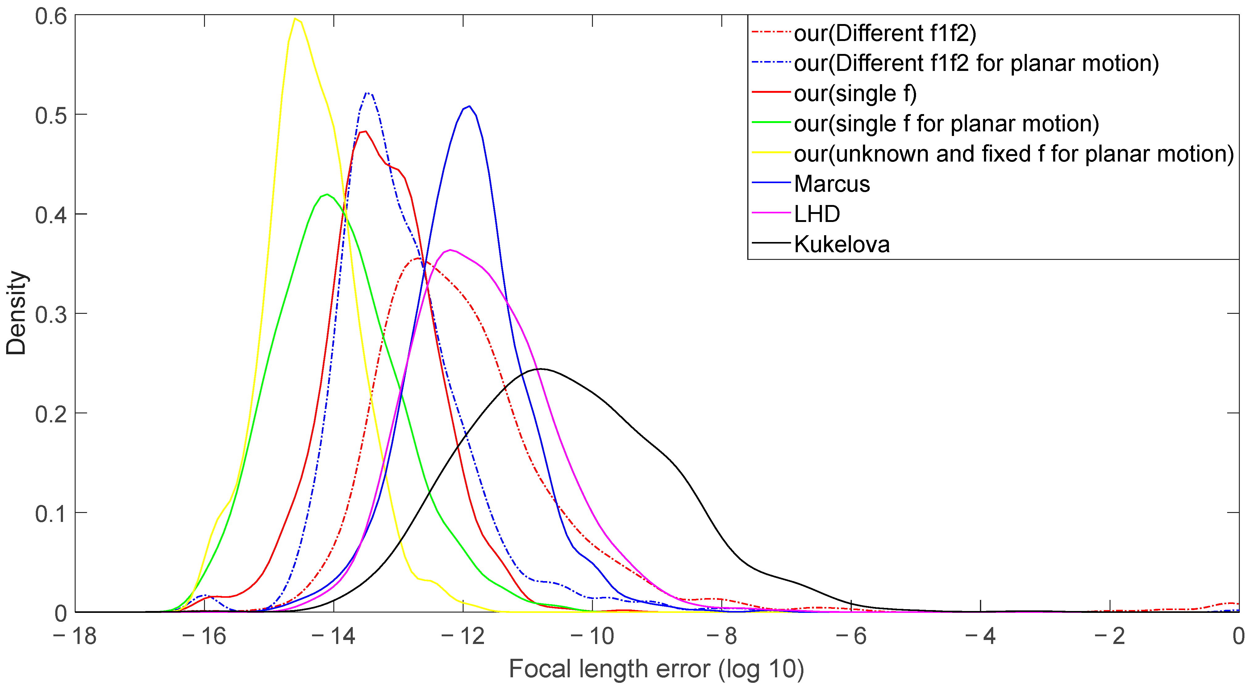
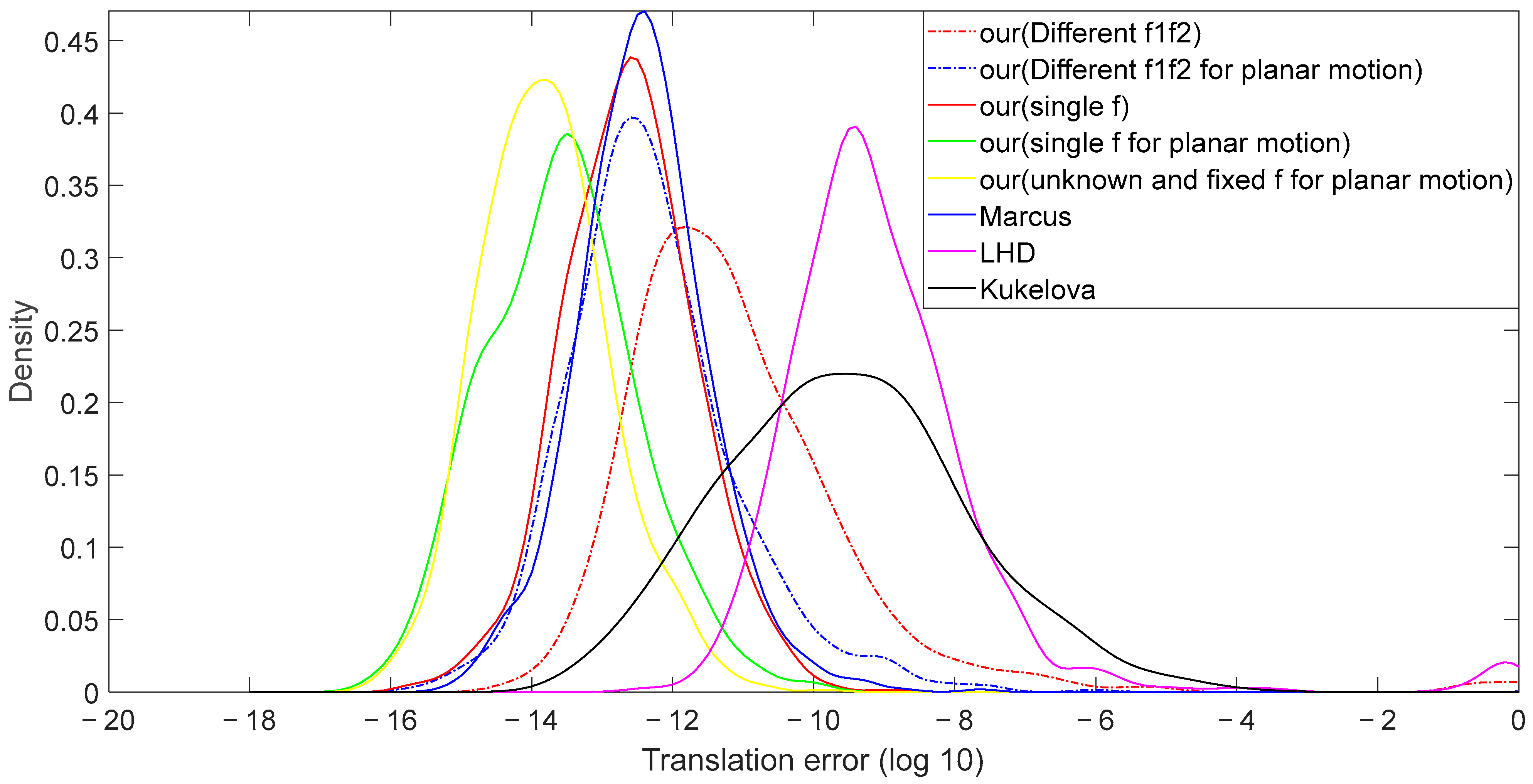
To obtain more realistic simulated data, we constructed a test scenario with randomly generated 3D points. Specifically, the scene points (X, Y, Z) were uniformly distributed with X, Z ∈ [−5, 5] m, the depth Y ∈ [10, 20] m, and the focal length f ∈ [100, 1000]. We set the resolution to 1000 × 700, and the principal point P0 = (500, 350) pixels. The predefined three-dimensional points were projected onto the camera image to obtain their pixel coordinates. We conducted experiments with 10,000 sets of feature point coordinates and statistically analyzed the errors in the focal length f and translation vector t without noise. The results are presented in Figure 2 and Figure 3. Figure 2 shows the focal length error probability density, while Figure 3 presents the translation vector error probability density.
In Figure 2 and Figure 3, the horizontal axes represent the logarithmically transformed results for the estimated focal length error and translation vector error, respectively, while the vertical axis represents the probability density. In Figure 2 and Figure 3, curves positioned farther to the left indicate smaller estimation errors, while higher peaks represent more concentrated estimation errors. It is evident from Figure 2 and Figure 3 that although all the methods can accurately estimate relative pose, the algorithm proposed in this paper achieves higher accuracy than the reference algorithm. Table 2 presents the median estimation errors of the focal length and translation vector, which were calculated separately for the five proposed algorithms and the reference algorithm using the same dataset. The error is slightly larger when cameras with unknown and different focal lengths undergo random motion. This is attributed to the fact that, unlike the reference algorithm, the camera we used has a variable focal length, thereby adding an extra parameter that needs to be computed.
After estimating the values of the focal length and translation vector, three-dimensional coordinate points were generated using simulated data, and the reprojection coordinates in the pixel coordinate system were calculated based on these points and the estimated values. Subsequently, these reprojection coordinates were compared with those calculated using accurate focal lengths and translation vectors to compute the reprojection error. Table 3 presents the mean reprojection error calculated over 10,000 experiments. From the table, it can be observed that the reprojection error obtained using the proposed algorithm for estimating the focal length and translation vector is smaller, indicating higher reprojection accuracy.
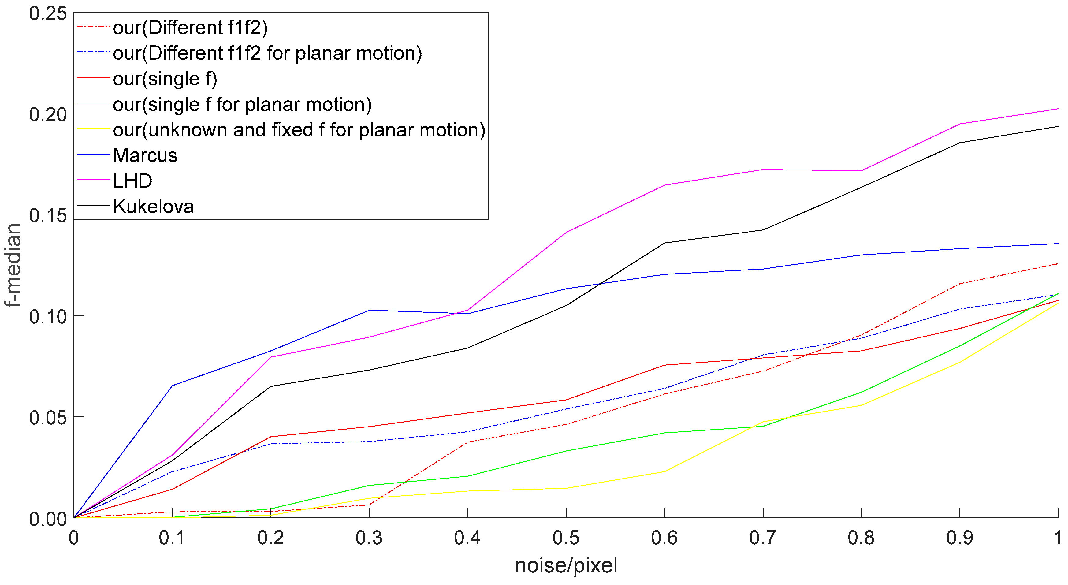
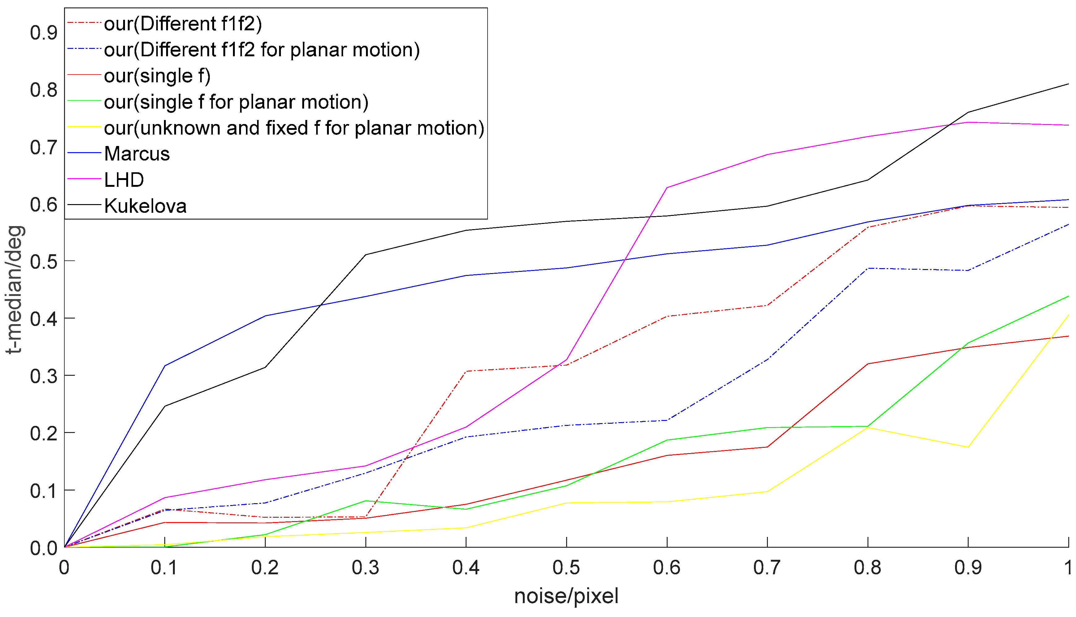
In practical applications, when estimating the relative pose of cameras, the first step involves extracting feature point correspondences. However, errors are inevitable during the feature point extraction process. To validate the performance of the proposed algorithm in the presence of errors in feature point coordinates, we conducted additional experiments, building upon the previous ones. We introduced random noise with coefficients ranging from 0 to 1 into the pixel coordinates of simulated points. Each model underwent ten thousand experiments, and the median errors of the focal length f and the translation vector t were calculated separately. The results are presented in Figure 4 and Figure 5.
In Figure 4 and Figure 5, it can be seen that the algorithm proposed in this paper yielded a higher accuracy focal length and translation vector than the contrast algorithm. The improvement was particularly significant when the pixel coordinate errors were small.
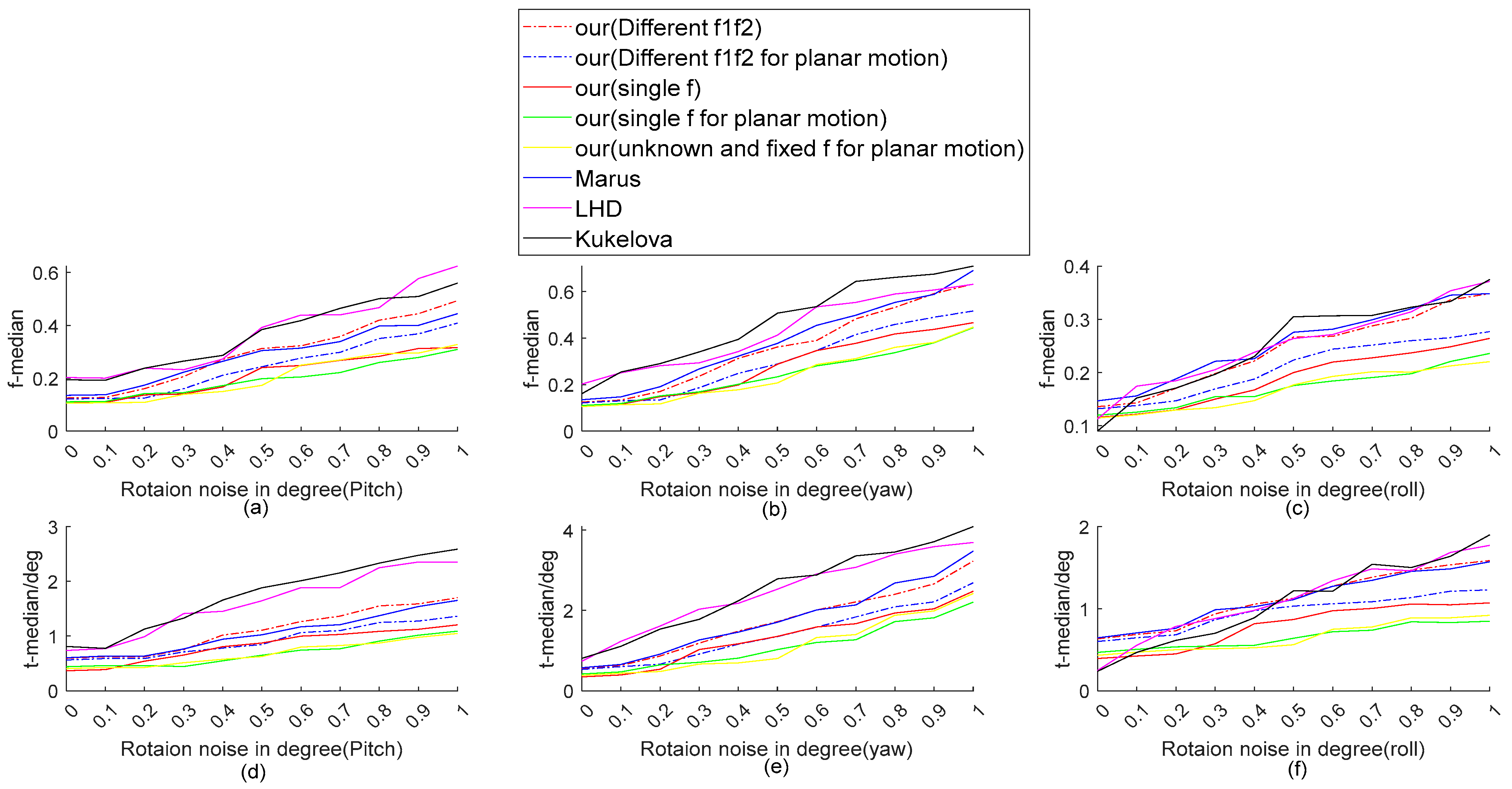
Although we utilized the rotation angles provided by the IMU as prior information, in real-life scenarios, due to variations in the performance of the IMU itself, the calculated rotation angles may exhibit errors of different scales. To further verify the performance of the proposed algorithm in the presence of IMU errors, we set up control experiments. Random noise with coefficients ranging from 0° to 1° was introduced into the three rotation angles, and random noise with a coefficient of 1 pixel was added to the image noise. The resulting errors in camera focal length and the relative translation vector were then calculated. The experimental results are presented in Figure 6. The first row shows the curve graph of camera focal length errors calculated using the different algorithms after introducing errors into the three angles, while the second row illustrates the curve graph of errors in the relative rotation matrix of the camera. Figure 6a,d represent the cases where pitch angle rotation errors were introduced; Figure 6b,e represent the cases where yaw angle rotation errors were introduced; Figure 6c,f represent the cases where roll angle rotation errors were introduced. From the figures, it can be observed that the algorithm proposed in this paper achieves higher accuracy than the benchmark algorithms. Specifically, the calculation error of the roll angle has the least impact on the relative pose and focal length of the camera.

4.2. Real Data

4.2.1. Data Description

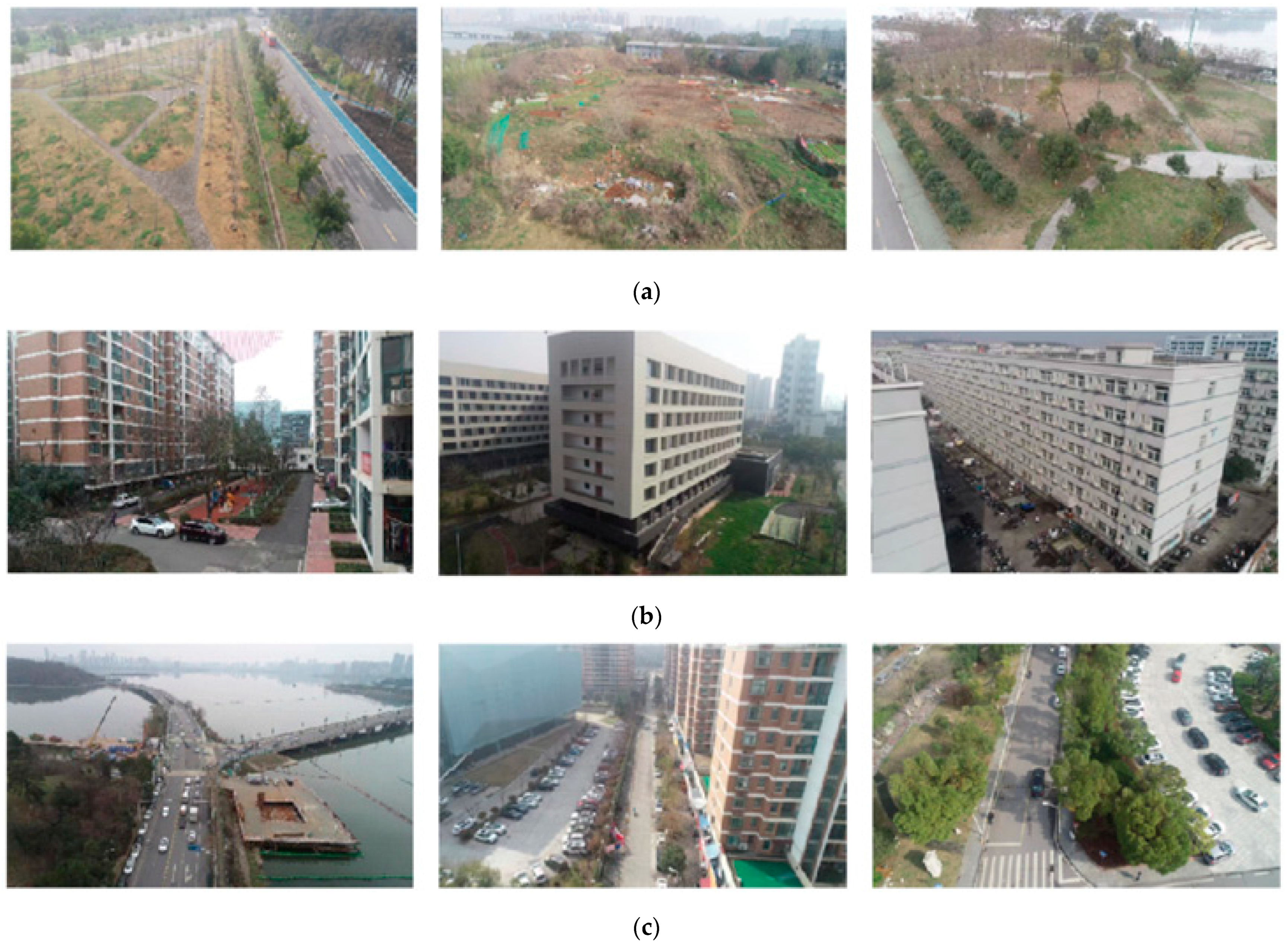
In order to more comprehensively test the performance of the algorithm proposed in this paper, images were captured using a drone in three different scenarios: outdoor landscapes, urban buildings, and road vehicles. The drone was equipped with Basler acA2040-120uc color cameras to capture the images. The drone was also equipped with an IMU module to obtain the rotation angles in three directions, and the IMU module was rigidly attached to the camera. Table 4 lists the common parameters of the IMU mounted on the drone. Before operating the drone, we ensured it remained stationary on the ground for a period of time. This allowed us to perform the initial calibration of IMU drift using the information obtained from the IMU outputs. We collected a total of 30,000 images from three different scenes to serve as the validation dataset for the algorithm. The reference value for the camera focal length was obtained through pre-calibration using the calibration board, while the reference value for the translation vector was calculated using the GNSS module mounted on the drone. We show example images from the scenes in Figure 7.
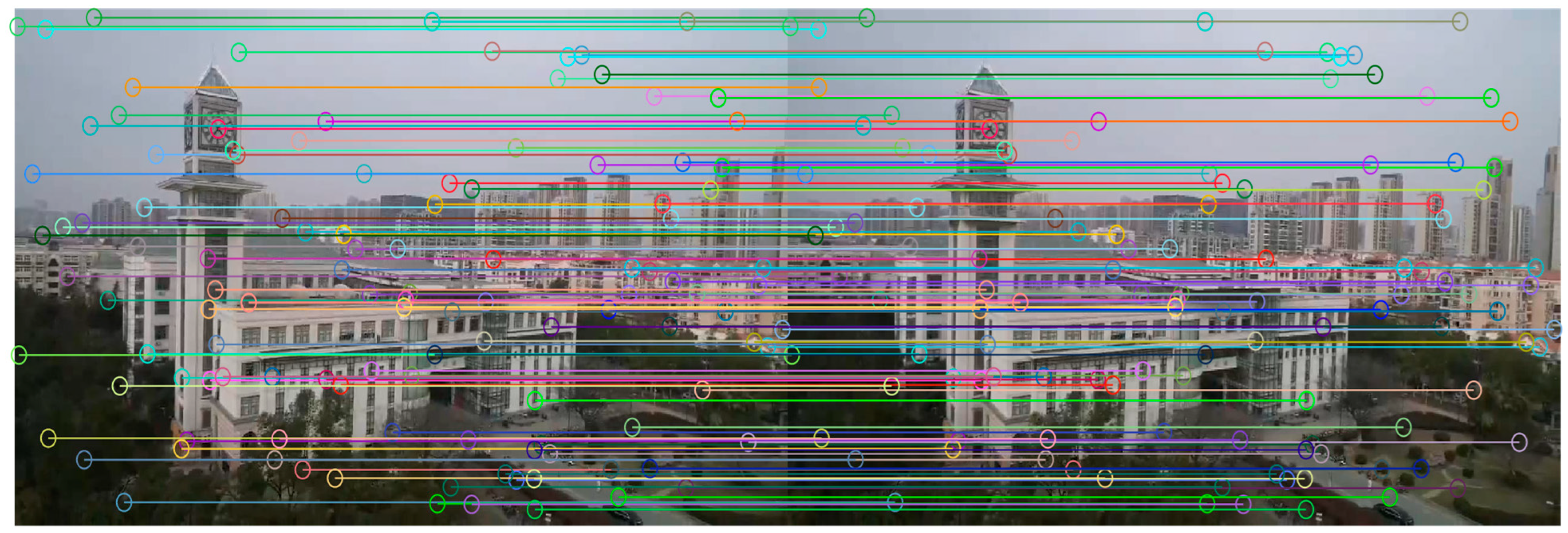
We synchronized the timestamps of the two cameras mounted on the drone using a GNSS to capture images from different cameras at the same time. We also obtained the 3D coordinates of the drone from the GNSS at that same moment, thus allowing us to calculate the reference value for the translation vector. After obtaining a sufficient number of image data along with corresponding reference values for the camera focal lengths and translation vectors, we used the SIFT algorithm to extract the corresponding coordinates of feature point pairs from frames captured at the same moment by different cameras [38]. Subsequently, we employed the RANSAC algorithm to evaluate the extracted feature points and eliminate those with significant errors [37]. As shown in Figure 8, the SIFT algorithm was used to extract corresponding feature points from the images. In order to achieve a clearer visualization of the extracted feature point pairs, every 20th feature point is marked in the schematic.

4.2.2. Relative Pose Analysis

We divided the collected dataset into three groups based on different data collection scenarios: Group 1 represents outdoor landscapes, Group 2 represents urban buildings, and Group 3 represents road vehicles. Each group of data was processed separately. We conducted statistical analysis on the errors in the focal length and translation vector as calculated using the algorithm proposed in this paper to validate its applicability. The median and standard deviation of the calculation errors are shown in Table 5. As shown in the table, in any given scenario, it is evident that the errors in both the estimated focal length and translation vector using our algorithm were smaller, and they further decreased as the complexity of the model decreased. The standard deviation of the algorithm proposed in this paper is comparatively smaller than that of the reference algorithm, which demonstrates the superior stability of our algorithm. Comparing the computational results across the three scenarios, the focal length and translation vector precision calculated from images captured in urban scenes were the highest, followed by those determined for road vehicle scenes, with the lowest estimation accuracy calculated for outdoor landscapes. This is because, in urban scenes, there are more regular objects in the captured images, resulting in smaller errors when extracting feature points.
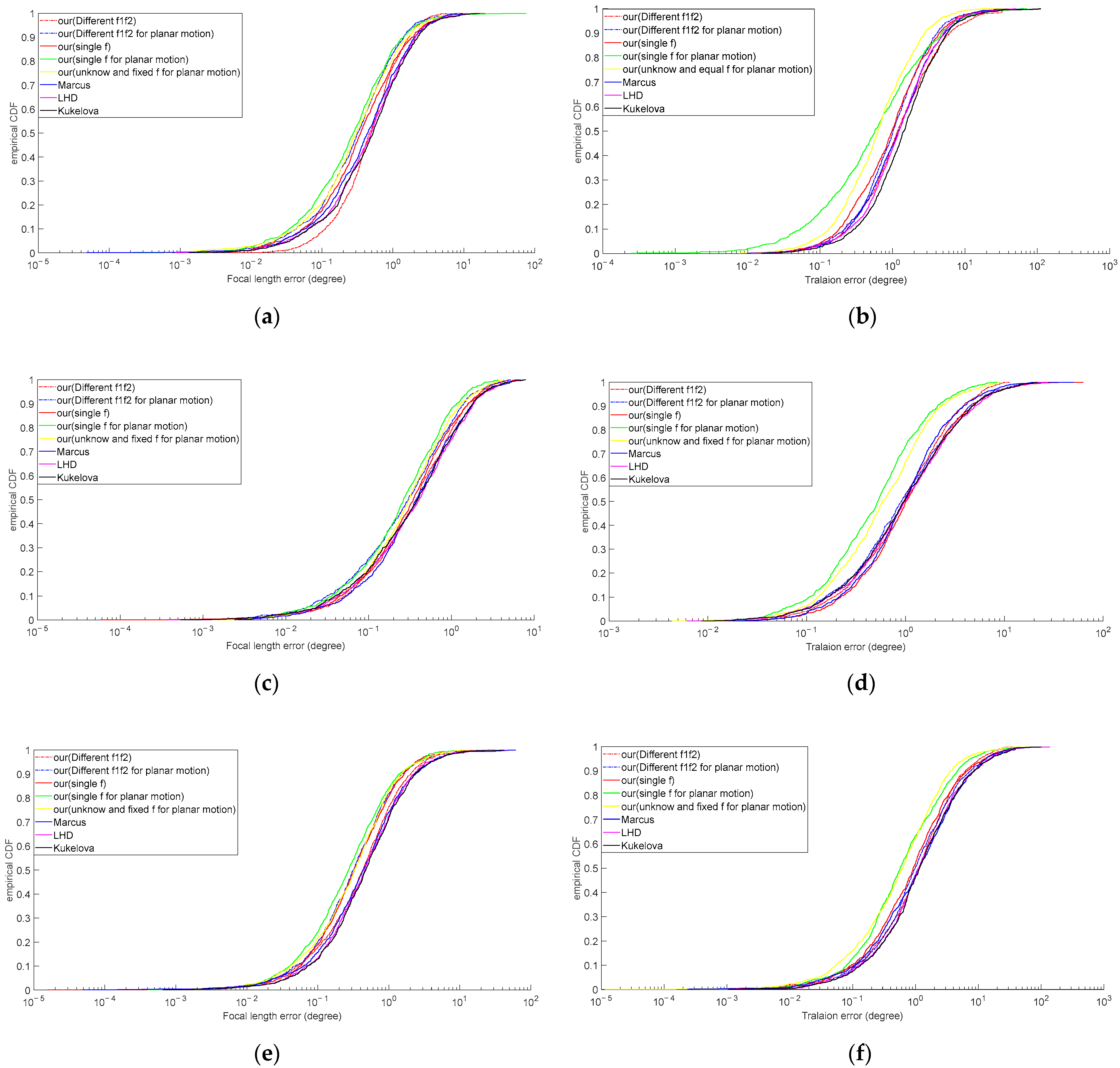
In order to better understand the errors in the calculated focal lengths and translation vectors across all images in the dataset, the cumulative distribution functions of the errors are presented for different scenarios. In Figure 9, the curves positioned farther to the left indicate smaller errors estimated by the model, while steeper slopes suggest a more concentrated range of errors. From the graph, it is evident that the algorithm proposed in this paper yields smaller estimation errors than the reference algorithm. Larger errors only occurred when calculating parameters for cameras with different and unknown focal lengths, which is attributed to the increased complexity of calculating additional parameters, aligning with the experimental results using simulated data.

4.2.3. Position Estimation Analysis

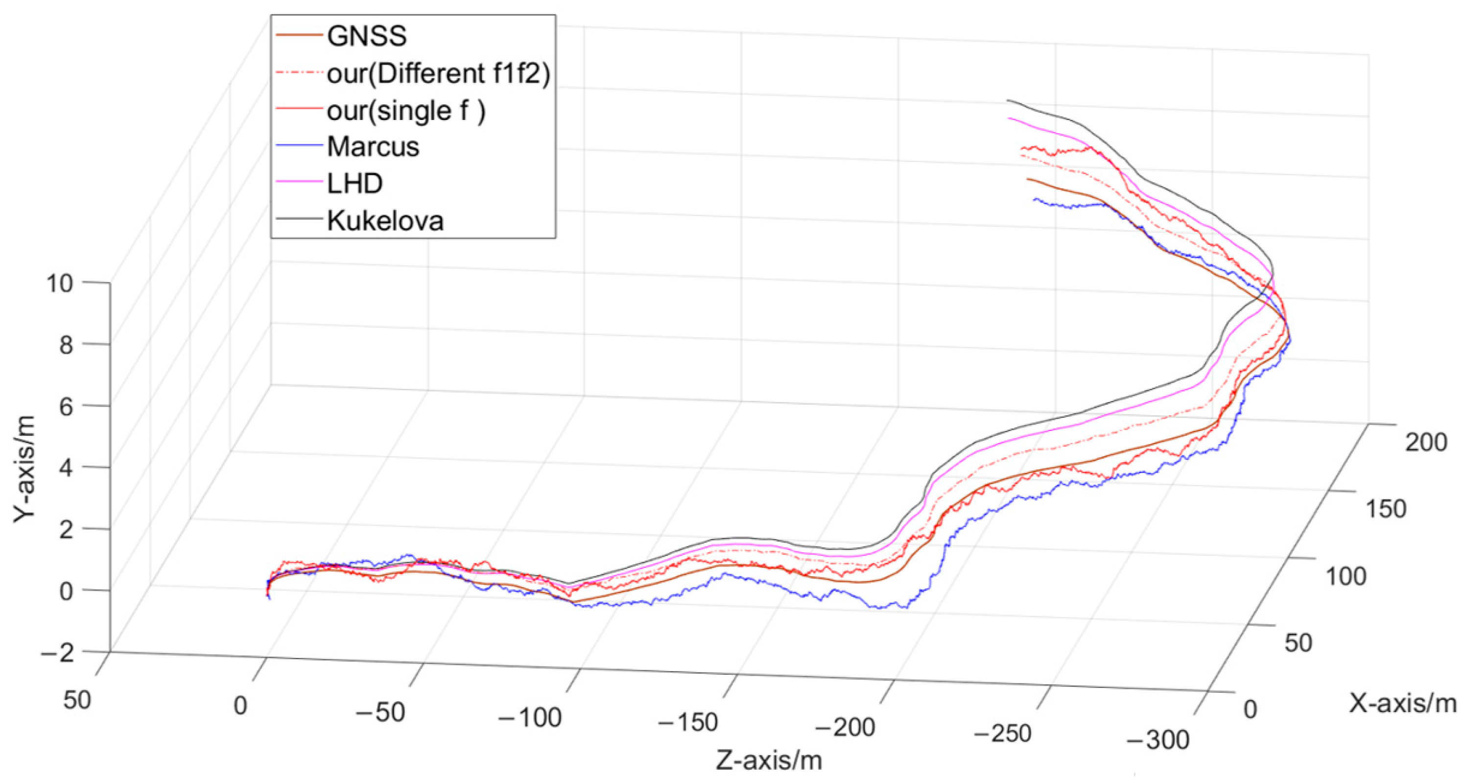
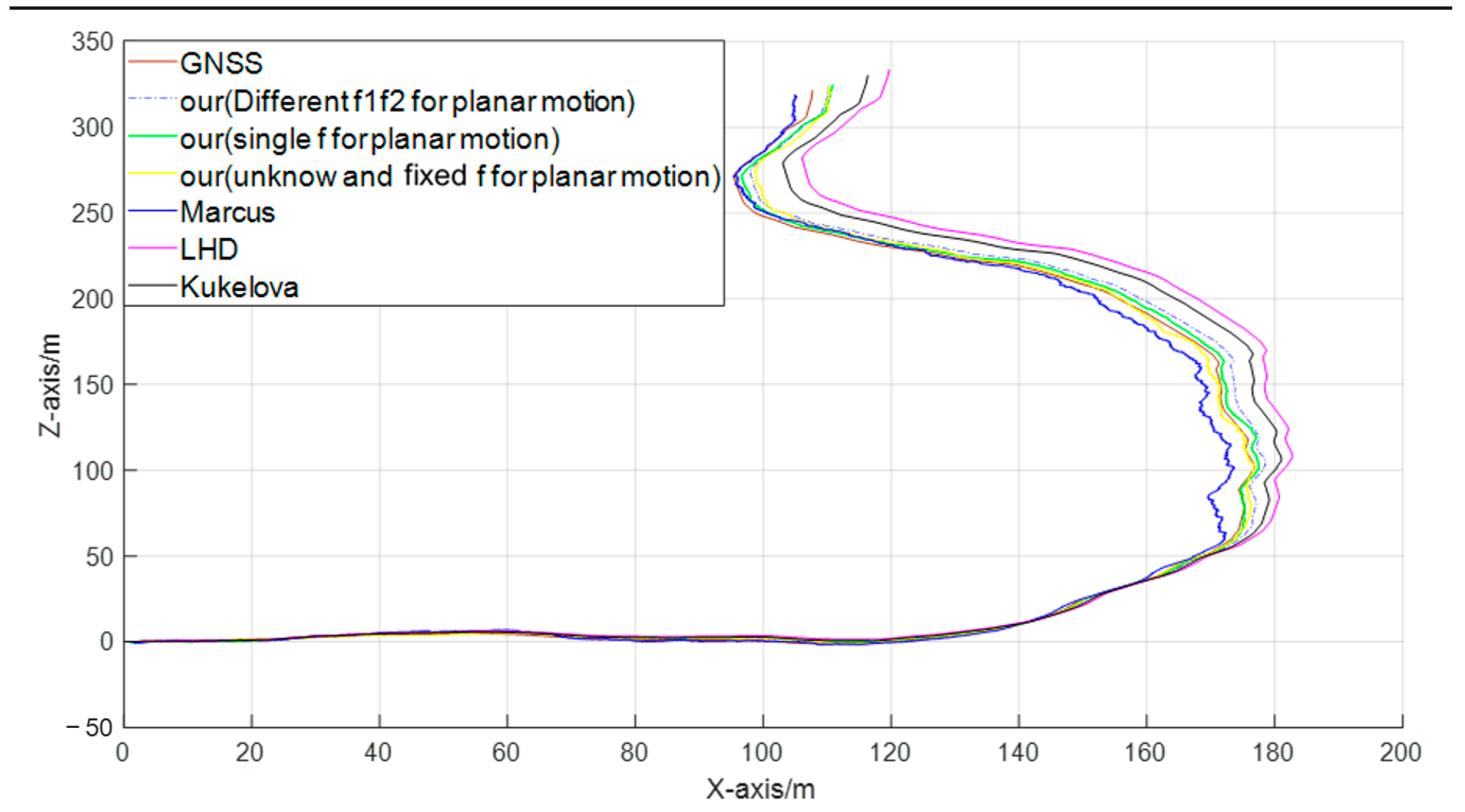
To visually assess the performance of various algorithms, two segments of data were extracted from the collected dataset and plotted on a trajectory graph. The trajectory graph uses GNSS positioning coordinates as reference ground truth. Since relative pose estimation lacks absolute positioning coordinates, the GNSS positioning result at the starting time was taken as the origin. Additionally, since none of the methods can estimate the scale correctly, the ground-truth scale was used to plot the trajectories. Since some of the algorithms proposed in this paper are based on planar motion, one segment of the trajectory consisted of data collected with the drone locked in the vertical direction. This segment was used to test the performance of algorithms based on planar motion. Figure 10 presents a 3D trajectory plot of random motion from measured data, while Figure 11 shows a 2D trajectory plot of planar motion. From the trajectory plots, it is evident that the algorithm proposed in this paper exhibited smaller errors than the reference algorithm when compared to the ground truth.

5. Conclusions

This paper presents four different methods of estimating relative pose and focal length in various application scenarios, aiming to enhance accuracy in addressing practical challenges. Given that the short-term drift of the IMU can be ignored, we calculated the rotation angles in three directions using IMU data. This reduces the number of feature point pairs required for relative pose and focal length estimation, thereby lowering the computational complexity of the relative pose estimation algorithm. The proposed algorithm was validated using both simulated data and real data collected from drones. The experiments demonstrated that, compared to the current state-of-the-art methods, the algorithm presented in this paper achieves higher accuracy in relative pose and focal length estimation, with gradual improvement as the model parameters are simplified.

Author Contributions

Conceptualization, K.Y. and H.Z.; methodology, K.Y. and Z.Y.; software, K.Y. and Z.Y.; validation, K.Y., C.S. and Z.Y.; formal analysis, D.C. and Z.Y.; investigation, K.Y. and Z.Y.; resources, Z.Y., D.C. and H.Z.; data curation, D.C. and C.S.; writing—original draft preparation, K.Y. and Z.Y.; writing—review and editing, K.Y. and Z.Y.; visualization, K.Y., C.S. and Z.Y.; supervision, D.C., H.Z. and C.S.; project administration, K.Y., Z.Y. and H.Z.; funding acquisition, H.Z. All authors have read and agreed to the published version of the manuscript.

Funding

This research was funded by the National Key Research and Development Program of China (No. 2021YFB2501104) and in part by the Ministry of Industry and Information Technology of China through the High-Precision Timing Service Project under grant TC220A04A-80 and in part by Major Program(JD) of Hubei Province(2023AA02604).

Data Availability Statement

The original contributions presented in the study are included in the article. Further inquiries can be directed to the corresponding author.

Acknowledgments

We would like to thank the editor and anonymous reviewers for their constructive comments and suggestions for improving the manuscript.

Conflicts of Interest

The authors declare no conflicts of interest.

References

  1. Wang, H.; Ban, X.; Ding, F.; Xiao, Y.; Zhou, J. Monocular VO Based on Deep Siamese Convolutional Neural Network. Complexity 2020, 2020, 6367273. [Google Scholar] [CrossRef]
  2. Wang, K.; Ma, S.; Chen, J.L.; Ren, F.; Lu, J.B. Approaches, Challenges, and Applications for Deep Visual Odometry: Toward Complicated and Emerging Areas. IEEE Trans. Cogn. Dev. Syst. 2022, 14, 35–49. [Google Scholar] [CrossRef]
  3. Chen, J.; Xie, F.; Huang, L.; Yang, J.; Liu, X.; Shi, J. A Robot Pose Estimation Optimized Visual SLAM Algorithm Based on CO-HDC Instance Segmentation Network for Dynamic Scenes. Remote Sens. 2022, 14, 2114. [Google Scholar] [CrossRef]
  4. Hao, G.T.; Du, X.P.; Song, J.J. Relative Pose Estimation of Space Tumbling Non cooperative Target Based on Vision only SLAM. J. Astronaut. 2015, 36, 706–714. [Google Scholar]
  5. Yin, Z.; Wen, H.; Nie, W.; Zhou, M. Localization of Mobile Robots Based on Depth Camera. Remote Sens. 2023, 15, 4016. [Google Scholar] [CrossRef]
  6. Barath, D.; Mishkin, D.; Eichhardt, I.; Shipachev, I.; Matas, J. Efficient Initial Pose-graph Generation for Global SfM. In Proceedings of the Computer Vision and Pattern Recognition, Nashville, TN, USA, 20–25 June 2021. [Google Scholar]
  7. Liang, Y.; Yang, Y.; Mu, Y.; Cui, T. Robust Fusion of Multi-Source Images for Accurate 3D Reconstruction of Complex Urban Scenes. Remote Sens. 2023, 15, 5302. [Google Scholar] [CrossRef]
  8. Kalantari, M.; Hashemi, A.; Jung, F.; Guedon, J.-P. A New Solution to the Relative Orientation Problem Using Only 3 Points and the Vertical Direction. J. Math. Imaging Vis. 2011, 39, 259–268. [Google Scholar] [CrossRef]
  9. Barath, D.; Toth, T.; Hajder, L. A Minimal Solution for Two-view Focal-length Estimation using Two Affine Correspondences. In Proceedings of the IEEE Conference on Computer Vision and Pattern Recognition, Honolulu, HI, USA, 21–26 July 2017; IEEE: Piscataway, NJ, USA, 2017. [Google Scholar]
  10. Mach, C.A.C. Random Sample Consensus: A paradigm for model fitting with application to image analysis and automated cartography. Commun. ACM 1981, 24, 381–395. [Google Scholar]
  11. Hajder, L.; Barath, D. Relative planar motion for vehicle-mounted cameras from a single affine correspondence. In Proceedings of the 2020 IEEE International Conference on Robotics and Automation (ICRA), Paris, France, 31 May–31 August 2020. [Google Scholar]
  12. Choi, S.-I.; Park, S.-Y. A new 2-point absolute pose estimation algorithm under planar motion. Adv. Robot. 2015, 29, 1005–1013. [Google Scholar] [CrossRef]
  13. Fraundorfer, F.; Tanskanen, P.; Pollefeys, M. A Minimal Case Solution to the Calibrated Relative Pose Problem for the Case of Two Known Orientation Angles. In European Conference on Computer Vision; Springer: Berlin/Heidelberg, Germany, 2010. [Google Scholar]
  14. Ding, Y.; Barath, D.; Yang, J.; Kong, H.; Kukelova, Z. Globally Optimal Relative Pose Estimation with Gravity Prior. In Proceedings of the IEEE/CVF Conference on Computer Vision and Pattern Recognition, Nashville, TN, USA, 20–25 June 2021. [Google Scholar]
  15. Ding, Y.; Yang, J.; Kong, H. An efficient solution to the relative pose estimation with a common direction. In Proceedings of the 2020 IEEE International Conference on Robotics and Automation (ICRA), Paris, France, 31 May–31 August 2020. [Google Scholar]
  16. Saurer, O.; Vasseur, P.; Boutteau, R.; Demonceaux, C.; Pollefeys, M.; Fraundorfer, F. Homography Based Egomotion Estimation with a Common Direction. IEEE Trans. Pattern Anal. Mach. Intell. 2017, 39, 327–341. [Google Scholar] [CrossRef] [PubMed]
  17. Sweeney, C.; Flynn, J.; Turk, M. Solving for Relative Pose with a Partially Known Rotation is a Quadratic Eigenvalue Problem. In Proceedings of the 2014 2nd International Conference on 3D Vision, Tokyo, Japan, 8–11 December 2014; IEEE: Piscataway, NJ, USA, 2014. [Google Scholar]
  18. Hartley, R.; Zisserman, A. Multiple View Geometry in Computer Vision, 2nd ed.; Cambridge University Press: Cambridge, UK, 2003. [Google Scholar]
  19. Li, H. A simple solution to the six-point two-view focal-length problem. In Computer Vision-ECCV 2006, Proceedings of the 9th European Conference on Computer Vision, Graz, Austria, 7–13 May 2006, Proceedings, Part IV 9; Leonardis, A., Bischof, H., Pinz, A., Eds.; Lecture Notes in Computer Science; Springer: Berlin/Heidelberg, Germany, 2006; Volume 3954, pp. 200–213. [Google Scholar]
  20. Hartley, R.; Li, H. An Efficient Hidden Variable Approach to Minimal-Case Camera Motion Estimation. IEEE Trans. Pattern Anal. Mach. Intell. 2012, 34, 2303–2314. [Google Scholar] [CrossRef] [PubMed]
  21. Stewenius, H.; Nister, D.; Kahl, F.; Schaffalitzky, F. A minimal solution for relative pose with unknown focal length. In Proceedings of the IEEE Computer Society Conference on Computer Vision & Pattern Recognition, San Diego, CA, USA, 20–25 June 2005. [Google Scholar]
  22. Bujnak, M.; Kukelova, Z.; Pajdla, T. 3D reconstruction from image collections with a single known focal length. In Proceedings of the IEEE International Conference on Computer Vision, Kyoto, Japan, 29 September–2 October 2009. [Google Scholar]
  23. Torii, A.; Kukelova, Z.; Bujnak, M.; Pajdla, T. The Six Point Algorithm Revisited. In Proceedings of the Computer Vision–ACCV 2010 Workshops: ACCV 2010 International Workshops, Queenstown, New Zealand, 8–9 November 2010. [Google Scholar]
  24. Kukelova, Z.; Bujnak, M.; Pajdla, T. Polynomial Eigenvalue Solutions to Minimal Problems in Computer Vision. IEEE Trans. Pattern Anal. Mach. Intell. 2012, 34, 1381–1393. [Google Scholar] [CrossRef] [PubMed]
  25. Hedborg, J.; Felsberg, M. Fast iterative five point relative pose estimation. In Proceedings of the 2013 IEEE Workshop on Robot Vision (WORV), Clearwater Beach, FL, USA, 15–17 January 2013. [Google Scholar]
  26. Kukelova, Z.; Kileel, J.; Sturmfels, B.; Pajdla, T. A clever elimination strategy for efficient minimal solvers. In Proceedings of the IEEE Conference on Computer Vision and Pattern Recognition, Honolulu, HI, USA, 21–26 July 2017. [Google Scholar]
  27. Bougnoux, S. From projective to Euclidean space under any practical situation, a criticism of self-calibration. In Proceedings of the International Conference on Computer Vision, Bombay, India, 4–7 January 1998. [Google Scholar]
  28. Hartley, R.I. Estimation of Relative Camera Positions for Uncalibrated Cameras. In Computer Vision—ECCV’92: Second European Conference on Computer Vision Santa Margherita Ligure, Italy, May 19–22, 1992 Proceedings 2; Springer: Berlin/Heidelberg, Germany, 1992. [Google Scholar]
  29. Li, H.; Hartley, R. A Non-Iterative Method for Correcting Lens Distortion from Nine Point Correspondences; OMNIVIS: South San Francisco, CA, USA, 2009. [Google Scholar]
  30. Jiang, F.; Kuang, Y.; Solem, J.E.; Åström, K. A Minimal Solution to Relative Pose with Unknown Focal Length and Radial Distortion; Springer International Publishing: Cham, Switzerland, 2015; pp. 443–456. [Google Scholar]
  31. Oskarsson, M. Fast Solvers for Minimal Radial Distortion Relative Pose Problems. In Proceedings of the IEEE/CVF Conference on Computer Vision and Pattern Recognition, Virtual, 19–25 June 2021; pp. 3663–3672. [Google Scholar]
  32. Rnhag, M.V.; Persson, P.; Wadenbck, M.; Strm, K.; Heyden, A. Trust Your IMU: Consequences of Ignoring the IMU Drift. In Proceedings of the IEEE/CVF Conference on Computer Vision and Pattern Recognition, New Orleans, LA, USA, 18–24 June 2022. [Google Scholar]
  33. Savage, P.G. Strapdown Analytics; Strapdown Associates: Maple Plain, MN, USA, 2000. [Google Scholar]
  34. Larsson, V.; Oskarsson, M.; Astrom, K.; Wallis, A.; Kukelova, Z. Beyond Grobner Bases: Basis Selection for Minimal Solvers. In Proceedings of the IEEE/CVF Conference on Computer Vision & Pattern Recognition, Salt Lake City, UT, USA, 18–23 June 2018. [Google Scholar]
  35. Stewénius, H.; Engels, C.; Nistér, D. An Efficient Minimal Solution for Infinitesimal Camera Motion. In Proceedings of the IEEE Conference on Computer Vision & Pattern Recognition, Minneapolis, MN, USA, 17–22 June 2007. [Google Scholar]
  36. Byrod, M.; Josephson, K.; Astrom, K. Fast and Stable Polynomial Equation Solving and Its Application to Computer Vision. Int. J. Comput. Vis. 2009, 84, 237–256. [Google Scholar] [CrossRef]
  37. Cardano, G.; Witmer, T.R.; Ore, O. The Great Art or the Rules of Algebra; Dover Publications: New York, NY, USA, 1968. [Google Scholar]
  38. Lowe, D.G. Distinctive Image Features from Scale-Invariant Key-points. Int. J. Comput. Vis. 2004, 60, 91–110. [Google Scholar] [CrossRef]
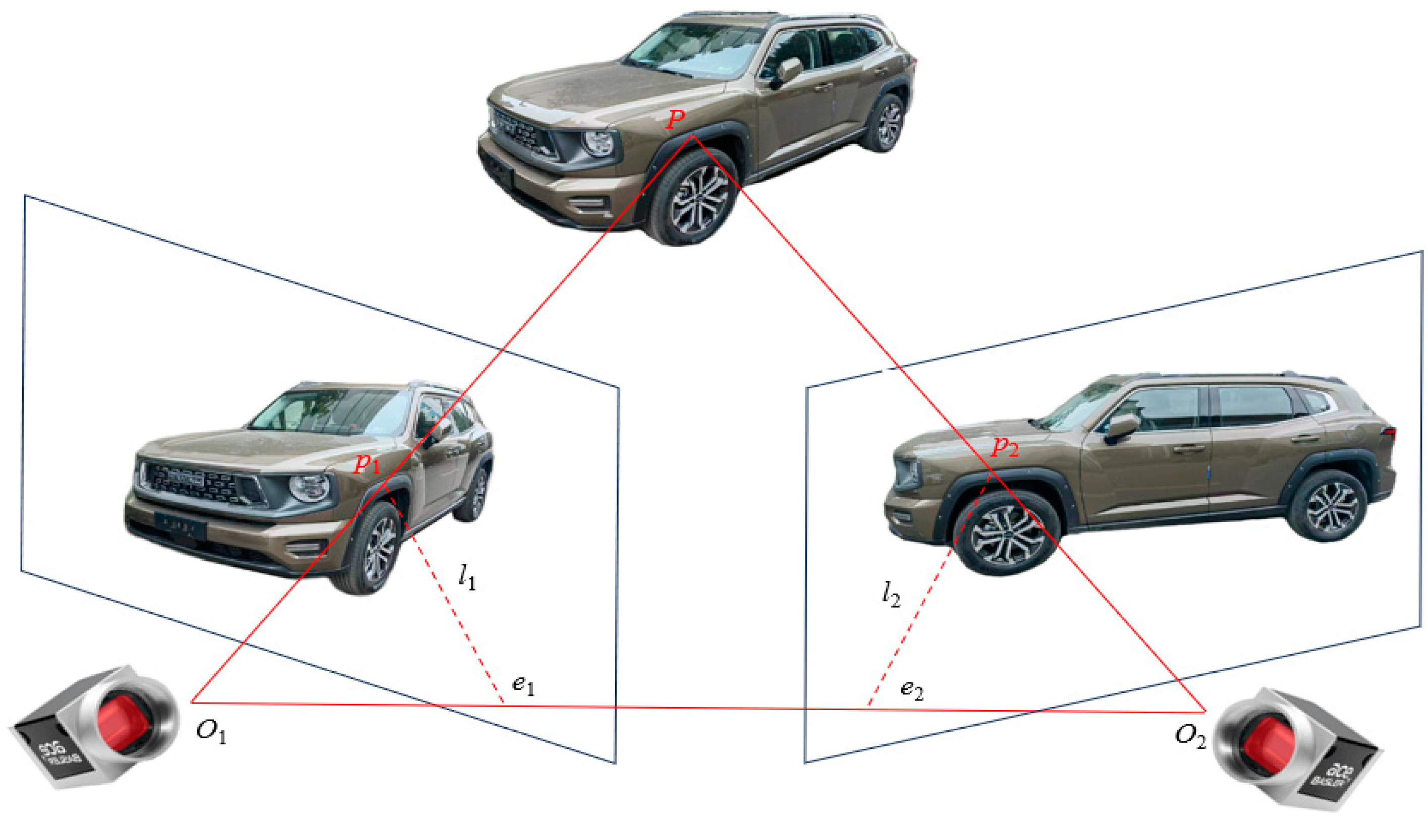
Figure 1. O1 and O2 represent the camera center; P denotes the target feature point; p1 and p2 are the pixel coordinates of the feature points; e1 and e2 are epipoles, which are the points where the line connecting O1 and O2 intersects with the image plane; O1, O2, and P forms the epipolar plane; and l1 and l2 are the epipolar lines, which are the lines where the epipolar plane intersects with the image plane.
Drones 08 00423 g001
Figure 2. Focal length error probability density for 10,000 randomly generated problem instances.
Drones 08 00423 g002
Figure 3. Translation matrix error probability density for 10,000 randomly generated problem instances.
Drones 08 00423 g003
Figure 4. Error variation curve of focal length f with different scale errors in pixel coordinates.
Drones 08 00423 g004
Figure 5. Error variation curve of translation vector t with different scale errors in pixel coordinates.
Drones 08 00423 g005
Figure 6. The error variation curves of eight methods when introducing different levels of noise into the three rotation angles with the IMU: (a) the median focal length error calculated after introducing pitch angle rotation errors; (b) the median focal length error calculated after introducing yaw angle rotation errors; (c) the median focal length error calculated after introducing roll angle rotation errors; (d) the median translation vector error calculated after introducing pitch angle rotation errors; (e) the median translation vector error calculated after introducing yaw angle rotation errors; (f) the median translation vector error calculated after introducing roll angle rotation errors.
Drones 08 00423 g006
Figure 7. Images captured by the drone: (a) outdoor landscapes; (b) urban buildings; (c) road vehicles.
Drones 08 00423 g007
Figure 8. Schematic of feature point extraction using the SIFT algorithm.
Drones 08 00423 g008
Figure 9. Cumulative distribution functions of the estimated errors in camera focal length and translation vector across three scenarios: (a) the camera focal length error of outdoor landscapes; (b) the translation vector error of outdoor landscapes; (c) the camera focal length error of urban buildings; (d) the translation vector error of urban buildings; (e) the camera focal length error of road vehicles; (f) the translation vector error of road vehicles.
Drones 08 00423 g009
Figure 10. Three-dimensional trajectory plot of real data.
Drones 08 00423 g010
Figure 11. Two-dimensional trajectory plot of real data.
Drones 08 00423 g011
Table 1. Parameterization for the different relative pose cases.
MethodsMinimum Points RequiredEstimated ParametersMotion Model
Different f1f24f1 f2 tRandom motion
Different f1f2 for planar motion3f1 f2 tPlanar motion
Single f3f tRandom motion
Single f for planar motion2f tPlanar motion
Unknown and fixed f for planar motion2f tPlanar motion
Table 2. The median estimation errors of the focal length f and translation vector t based on simulated data.
ξ f -Median/Pixel ξ t -Median/Deg
Marcus [32]1.1023 × 10−133.7090 × 10⁻¹³
LHD [19]1.6473 × 10−125.3201 × 10⁻¹⁰
Kukelova [24]3.1238 × 10−112.3635 × 10⁻¹⁰
Different f1f21.3707 × 10−134.0739 × 10⁻¹³
Different f1f2 for planar motion7.8180 × 10−159.6702 × 10⁻¹⁴
Unknown and fixed f for planar motion1.3309 × 10−153.6772 × 10⁻¹⁵
Single f9.8511 × 10−153.0763 × 10⁻¹⁴
Single f for planar motion1.5763 × 10−153.5108 × 10⁻¹⁶
Table 3. The median reprojection errors with the eight algorithms.
Reprojection Error/Pixel
Marcus [32]8.1885 × 10⁻¹³
LHD [19]3.2519 × 10⁻¹²
Kukelova [24]5.8134 × 10⁻¹¹
Different f1f27.8529 × 10−13
Different f1f2 for planar motion5.2568 × 10−14
Unknown and fixed f for planar motion7.7419 × 10−15
Single f4.1573 × 10−14
Single f for planar motion6.8135 × 10−15
Table 4. IMU parameters carried by drone.
ParameterValue
GyroscopeRange±300°/s
Angular random walk0.1 deg/√h
In-run bias stability0.5 deg/h
Bias repeatability0.5 deg/h
Scale factor error300 ppm
AccelerometerRange±10 g
In-run bias stability0.3 mg
Bias repeatability0.3 mg
Scale factor error300 ppm
Table 5. The median estimation errors of the focal length f and translation vector t based on real data.
123
ξ f ξ t ξ f ξ t ξ f ξ t
Marcus [32]Median0.44231.21260.38450.98420.43521.1189
SD2.51184.62142.79784.31543.26844.9851
LHD [19]Median0.49471.23420.41531.00590.45851.1216
SD3.82735.10564.31586.65174.56278.6149
Kukelova [24]Median0.52531.43520.39750.98180.47371.1587
SD4.86287.51573.51598.31733.97915.9004
Different f1f2Median0.47071.17390.38090.96470.43361.1358
SD2.48913.42392.35132.90582.61253.2268
Different f1f2 for planar motionMedian0.31731.02080.30470.91550.31590.9853
SD2.10412.85182.23182.65172.33613.0156
Unknown and fixed f for planar motionMedian0.30580.63470.31140.59190.29310.6241
SD1.91942.12732.01812.31581.91802.2368
Single fMedian0.35130.97660.35051.01830.32690.9186
SD1.81082.25391.91732.15861.76891.9627
Single f for planar motionMedian0.27610.57060.26540.52860.27190.5697
SD1.49311.68171.41681.88171.52171.8136
Disclaimer/Publisher’s Note: The statements, opinions and data contained in all publications are solely those of the individual author(s) and contributor(s) and not of MDPI and/or the editor(s). MDPI and/or the editor(s) disclaim responsibility for any injury to people or property resulting from any ideas, methods, instructions or products referred to in the content.