Collaborative Obstacle Detection for Dual USVs Using MGNN-DANet with Movable Virtual Nodes and Double Attention

Abstract

To reduce missed detections in LiDAR-based obstacle detection, this paper proposes a dual unmanned surface vessels (USVs) obstacle detection method using the MGNN-DANet template matching framework. Firstly, point cloud templates for each USV are created, and a clustering algorithm extracts suspected targets from the point clouds captured by a single USV. Secondly, a graph neural network model based on the movable virtual nodes is designed, introducing a neighborhood distribution uniformity metric. This model enhances the local point cloud distribution features of the templates and suspected targets through a local sampling strategy. Furthermore, a feature matching model based on double attention is developed, employing self-attention to aggregate the features of the templates and cross-attention to evaluate the similarity between suspected targets and aggregated templates, thereby identifying and locating another USV within the targets detected by each USV. Finally, the deviation between the measured and true positions of one USV is used to correct the point clouds obtained by the other USV, and obstacle positions are annotated through dual-view point cloud clustering. Experimental results show that, compared to single USV detection methods, the proposed method reduces the missed detection rate of maritime obstacles by 7.88% to 14.69%.

1. Introduction

With the ongoing advancement and preservation of coastal ocean resources, un-manned surface vessels (USVs) have become increasingly indispensable for tasks such as water quality monitoring, coastal patrolling, and search and rescue operations. This is due to their autonomy, high safety standards, and ability to operate continuously [1,2,3,4]. However, in the coastal ocean environment, numerous obstacles, including reefs, fishing boats, and small floating objects, pose significant threats to the safety of USVs. Traditional image sensors only capture two-dimensional information, which limits the effectiveness of visual methods for directly locating obstacles [5,6,7]. In contrast, LiDAR provides precise positional information, facilitating more accurate obstacle detection [8,9,10]. However, LiDAR-based methods require a high quantity of point clouds in the obstacle region. Some obstacles, due to their size or the angle of observation, may reflect fewer point clouds, making them difficult to detect with LiDAR [11].

In the challenging marine environment, characterized by strong winds, waves, and currents, USVs experience rapid and substantial swaying, making it difficult for a low-cost Inertial Measurement Unit (IMU) to provide real-time, accurate pose information. This swaying causes the point clouds obtained by the two vessels to rotate within the geodetic coordinate system, leading to deviations from the true positions of obstacles. Consequently, effectively reducing missed detections in dual USV systems is challenging until the issue of point cloud deviation caused by swaying is addressed.

As dual USV formations become more widely applied, dual vessels positioned at different locations can provide a greater quantity of point clouds describing the surrounding objects. However, it is crucial to emphasize that the overall increase in point cloud quantity does not directly correspond to a rise in the quantity of point clouds within the region where obstacles are situated. This is due to the inherent limitations of USVs, which are typically low cost and compact, with dimensions ranging from 1 to 2 m [12,13]. In the challenging marine environment, characterized by strong winds, waves, and currents, USVs experience rapid and substantial swaying, making it difficult for a low-cost Inertial Measurement Unit (IMU) to provide real-time, accurate pose information. In such conditions, the point clouds acquired by the two vessels undergo rotations in the geodetic coordinate system, causing the obstacle point cloud to deviate from its true position. This results in the inability to directly augment the quantity of point clouds within the obstacle regions. Therefore, effectively reducing missed detections by dual USVs is impeded until the issue of point cloud deviation caused by swaying is addressed.

2. Related Work

This section reviews the prevailing methods and technologies for correcting point cloud positional deviations, with a focus on point cloud registration methods that use coastal point clouds as references and template matching methods that rely on mutual references between dual USVs to correct point clouds. Additionally, it discusses the unique challenges faced by template matching methods in marine environments, particularly when coastal point clouds are unavailable, and highlights the main contributions of this paper in addressing these challenges.

2.1. Point Cloud Registration Methods

The predominant approach to rectifying position offsets in dual-view point clouds involves estimating rotational angles (pitch, roll, and yaw) by dual-view point clouds registration to align them. Clearly, with accurate rotation centers for the rotation of dual-view point cloud, the aligned point clouds through rotation will be in their true positions. At this point, the aggregation effect of point clouds from the same target observed by the two vessels reaches its optimum. They mainly include iterative optimization methods constrained by the positions of manually designed features and transformation parameter estimation methods based on deep learning.

In the realm of iterative optimization methods constrained by the positions of manually designed features, researchers initially extract key features from point clouds. These methods then employ iterative optimization techniques to minimize the distance between corresponding features in dual-view point clouds, facilitating alignment. Feature design is heavily reliant on human cognition of target characteristics, encompassing features such as the center of point clouds [14], 2-D silhouettes [15], local point-pair features [16], normal features [17], as well as the density, curvature, and normal angle of the target [18]. Iterative optimization methods commonly adopt improvements to traditional algorithms, such as the Hungarian algorithm [19] and the Iterative Closest Point (ICP) algorithm [20,21]. With the advent of deep learning, some scholars have integrated deep learning models into certain or all stages of traditional methods, leading to the development of transformation parameter estimation methods based on deep learning. For example, Xie et al. [22] proposed a convolutional Siamese point net (CSPN) to extract multiscale features from point clouds. Sun et al. [23] fused multilayer perceptron and graph neural network to extract deep features from point clouds. In contrast, Yi et al. [24] entrusted both feature extraction and iterative optimization entirely to deep learning models. Table 1 summarizes the mentioned point cloud registration methods.

Table 1. Comparison of the point cloud registration methods.

Methods	Extracted Key Features	Iterative Optimization Techniques
iterative optimization methods constrained by the positions of manually designed features	the center of point clouds [14], 2-D silhouettes [15], local point-pair features [16], nor-mal features [17], the density, curvature, and normal angle of the target [18]	the Hungarian algorithm [19], the Iterative Closest Point (ICP) algorithm [20,21]
transformation parameter estimation methods based on deep learning	multiscale features [22], deep features [23], global features [24]	singular value decomposition [22], nearest point matching and RANSAC [23], multilayer perceptron [24]

It is noteworthy that limited research exists on point cloud registration in marine environments, as most methods have been developed for terrestrial settings. Furthermore, these methods impose specific requirements regarding point cloud density. In the marine environment, obtaining dense point clouds as required for point cloud registration methods often depends on the visibility of coastal point clouds. However, when USVs are positioned far from shore, these point clouds become either invisible or extremely sparse. In such scenarios, each USV can only acquire point clouds of obstacles and its collaborative USV, making point cloud registration methods less effective.

2.2. Template Matching Methods

When coastal point clouds are unavailable, a feasible approach involves estimating the sway angles of the USV by analyzing the difference between the actual and measured positions of collaborative USV. Rotating all point clouds using these sway angles aligns them with their true positions. Notably, the accurate measurement of the real positions of dual USVs can be achieved using Global Navigation Satellite Systems (GNSS). While LiDAR-based detection methods can provide the positions of nearby targets, identifying the collaborative USV among these targets remains a general challenge. Therefore, identifying the collaborative USV from surrounding targets is key to correcting point cloud positions and minimizing obstacle detection misses, typically achieved through template matching methods.

In this paper, template matching refers to using point cloud data as a basis, with the point cloud of the object of interest serving as the template to search for instances of that object within a set of targets. These methods refine optimal results by evaluating feature similarities between the template and the targets. Ding et al. [25] implemented template matching based on the Signature of Histograms of Orientations (SHOT) feature and Ensemble of Shape Functions (ESF) feature, coupled with Hough voting. CMT [26] devised a horizontally rotation-invariant contextual descriptor to address potential rotation occurrences of the template and target. Yu et al. [27] employed the fast point feature histograms (FPFH) feature descriptor to characterize the local appearance of the target, achieving the best matching results through assessing both feature and geometric dissimilarities between the template and scene feature points. With the advancement of deep learning, some researchers have encoded point cloud data into high-dimensional vectors to represent latent features [28] and assessed the similarity between template and target using cosine similarity [29,30] or cross-correlation [31].

As application scenarios have diversified, researchers have found that sparse point clouds make it challenging to extract robust point cloud features. To enhance feature quality, targeted improvements to the feature extraction network are necessary based on the point cloud distribution characteristics of the research objects. PTT-Net [32] employs a self-attention network to capture global semantic features while retaining local context information of the point cloud. PTTR [33] introduces relation-aware sampling in PointNet++, obtaining higher-quality features by preserving more points related to the given template. 3DST [34], utilizing an attention network, captures the shape context feature of the target through non-local feature embedding and adaptive feature interpolation. Feng et al. [35] utilize a simplified PointNet and multistage self-attention to capture non-local context information of the point cloud. Regarding feature similarity measurement, both cosine similarity and cross-correlation are essentially linear matching processes, which are insufficient for adapting to complex situations involving random noise, occlusions, and rotation. To address this, PTTR [33] uses self-attention to adaptively aggregate features for the template and the target, followed by feature matching with cross-attention. Feng et al. [35] employ cross-attention to assess feature correlation between the template and the search area. However, there is currently a lack of template matching methods specifically designed for maritime vessels. Table 2 summarizes the mentioned template matching methods.

Table 2. Comparison of the template matching methods.

Methods	Core Concept	References	Technicalities
Traditional methods	Evaluating feature similarities between the template and the targets to refine optimal results	[25]	SHOT and ESF + Hough voting
		[26]	horizontally rotation-invariant contextual descriptor + shifted windows
		[27]	FPFH + convex optimization
		[28]	high-dimensional vectors + MLP
		[29,30]	high-dimensional vectors + cosine similarity
		[31]	high-dimensional vectors + cross-correlation
Deep learning methods	Constructing improved deep learning models to replace traditional feature extraction and similarity assessment	[32]	self-attention network
		[33]	PointNet++ with relation-aware sampling + cross-attention
		[34]	Siamese point transformer network + correlation network
		[35]	simplified PointNet and multistage self-attention + cross-attention

2.3. Challenges of Template Matching Methods

Using template matching methods to identify collaborative USVs from targets encounters two challenges in the maritime environment.

First, collaborative USVs and ships exhibit similar global shapes, with significant differences concentrated in focus regions like masts, where substantial shape variations occur locally. However, current template matching methods struggle to effectively pinpoint these focus regions and capture localized information, resulting in suboptimal matching performance.

Second, the rotation of maritime objects is inevitable, and shipborne LiDAR can only capture point clouds from one side of an object. The templates used in template matching are typically singular, encompassing point cloud distribution information from only one side of the collaborative USV. In practical application, the point clouds of collaborative USV may deviate significantly from the template. To ensure successful matching for collaborative USV with different orientations, it is necessary to simultaneously employ point clouds from different sides of the collaborative USV as templates. However, the number of templates is limited, while the potential rotation angles of the targets are infinite. Therefore, the challenge lies in how to aggregate a limited number of templates reflecting the point cloud distribution features from different sides of the collaborative USV and effectively use the aggregated template to identify the collaborative USV from the targets.

2.4. Contributions

In our paper, the main contributions are as follows:

(1)

Advanced Collaborative Obstacle Detection Method

This paper introduces a novel method for obstacle detection in dual USVs using a combination of movable virtual nodes and a double attention mechanism. This method significantly reduces missed detections by correcting the point cloud position deviations caused by the swaying of USVs. Unlike traditional methods, which rely heavily on shore-based references, this approach leverages the mutual positioning of two USVs as reference points for each other, offering a robust solution even in sparse point cloud environments, which is crucial for maritime operations.

(2)

Innovative feature extraction with movable virtual nodes

A unique feature extraction model based on movable virtual nodes is proposed, which enhances the local point cloud distribution features. This model integrates the uniformity of point cloud distribution within the vicinity of virtual nodes into the loss function, ensuring that the model directs attention toward critical focus regions. This approach not only realizes the extraction of point cloud distribution features but also enhances the effectiveness of point cloud processing by focusing on and accurately capturing critical features that might otherwise be missed.

(3)

Double attention-based feature matching

A double attention-based feature matching model is proposed to identify cooperative USV from marine targets. This model aggregates point cloud distribution features from multiple templates and employs cross-attention to evaluate the similarity between the aggregated template and detected targets. This method addresses the challenge of accurately identifying and matching collaborative USV in complex marine environments, where traditional single-perspective matching methods often fail.

3. Methodology

3.1. Overview

Our research aims to enhance obstacle detection by increasing the number of point clouds within regions where obstacles are located. This is achieved by using data collected from two USVs positioned differently and rectifying the point cloud rotation caused by the USVs’ swaying. Figure 1 illustrates a schematic representation of the process on a two-dimensional plane.

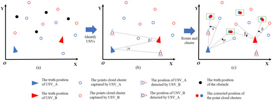
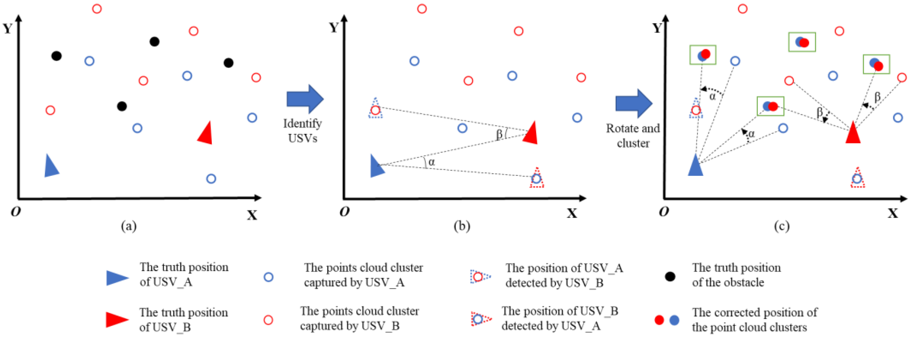
Figure 1. The process of correcting point cloud positions to increase the quantity of obstacle point clouds. (a) the point cloud cluster with displacement; (b) calculating the swaying angle; (c) correction and clustering.

In Figure 1a, the swaying motion of the USVs causes the point clouds captured by the LiDAR to rotate around the USV’s position, resulting in the displacement of point cloud clusters from their true positions. This displacement hinders the augmentation of obstacle point cloud quantity, thereby reducing the effectiveness of collaborative obstacle detection by the two USVs. To address this issue, our method identifies the other USV among the targets detected by a single USV, allowing for the computation of the USVs’ precise swaying angles. As depicted in Figure 1b, α and β represent the swaying angles of the two USVs in the XOY plane. Subsequently, the same rotation angle is applied to other point cloud clusters, repositioning them to their actual locations as illustrated in Figure 1c. This process increases the quantity of point clouds in the target area, and the application of clustering methods effectively resolves the issue of insufficient obstacle point clouds, which could lead to missed detections. It’s important to note that Figure 1 illustrates only the yaw angle correction process of the USVs, whereas our proposed method corrects the target point clouds’ positions in three dimensions: yaw, pitch, and roll.

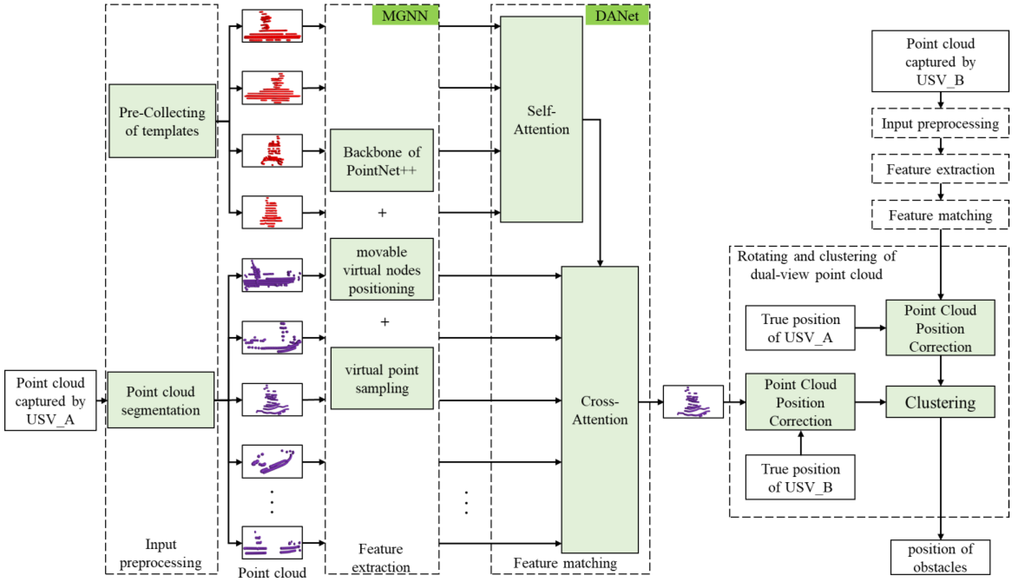
To achieve this goal, we have designed an obstacle detection method for dual USVs based on movable virtual nodes and double attention. The proposed method consists of four stages: input preprocessing, feature extraction, feature matching, and rotating and clustering of dual-view point cloud, as depicted in Figure 2. It is crucial to emphasize that the collaborative relationship between the two vessels is mutual, and the two sets of point clouds captured by the two USVs must undergo processing through these four stages separately.

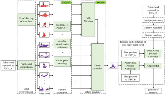
Figure 2. The overall architecture of the proposed obstacle detection method for dual USVs.

The input preprocessing stage consists of template preparation and rough point cloud segmentation. During template preparation, point clouds are pre-collected from all four sides of the collaborative USV to serve as templates. In the rough point cloud segmentation step, targets are preliminarily segmented from the point clouds acquired by the single USV. It is important to note that these targets include not only the collaborative USV but also an unspecified number of sea obstacles.

In the feature extraction stage, we design a graph neural network with the movable virtual nodes called MGNN to capture the point cloud distribution features of both targets and templates. MGNN integrates the backbone of PointNet++ with movable virtual nodes positioning and virtual point sampling to identifies focus regions, ensuring the enhancement of local information in these regions within the extracted features.

In the feature matching stage, we developed a feature matching model using a double attention network (DANet) to identify and locate the collaborative USV among the targets detected by the USV. This model incorporates self-attention as the first layer to aggregate the point cloud distribution features of the four templates. Subsequently, it employs cross-attention as the second layer to assess the similarity between the target and the templates, providing matching results.

In the dual-view point cloud rotation and clustering stage, we leverage the collaborative USV’s measured position and the actual position provided by GNSS to estimate the USV’s swaying angle. Due to the reciprocal relationship between the two vessels, this method can estimate the swaying angle for both USVs. The acquired swaying angles are then used to correct the positions of the point clouds obtained by the dual vessels. Finally, clustering is performed on the spatially corrected dual-view point cloud to derive obstacle detection results.

3.2. Input Preprocessing

Unlike terrestrial environments, the calm sea surface does not generate point clouds; only obstacles and waves do, resulting in sparse point clouds in marine settings. Directly applying deep learning models to such sparse data presents significant challenges. This approach would leave many neurons without the necessary information for effective learning, leading to poor model performance. Therefore, our proposed method does not directly search for the collaborative USV in all point clouds captured by a single USV. Instead, it conducts rough point cloud segmentation on the data acquired by a single USV to identify target candidates for the template matching method. Specifically, we utilize the Density-Based Spatial Clustering of Applications with Noise (DBSCAN) algorithm to segment point clouds corresponding to different targets. Clustering methods make the input point clouds denser, which aids the model in extracting more effective distribution features from the point clouds.

The observed side of a moving collaborative USV is unpredictable, and a single template from a fixed perspective may differ significantly from the point cloud of the collaborative USV. This poses a substantial challenge in matching the collaborative USV within the acquired point cloud. To address this issue, we prepare four templates during the template preparation stage. Specifically, we use LiDAR to collect point cloud data from the front, rear, left, and right sides of the collaborative USV in calm seas, creating four distinct templates. At this stage, the point cloud distribution relationships from any side of the USV are covered by these four templates without redundancy. It is important to note that template preparation and rough point cloud segmentation do not occur simultaneously. While rough point cloud segmentation takes place during the USV’s navigation, the templates are pre-prepared and do not require replacement.

3.3. Feature Extraction

Given the similarity in global point cloud distribution between the collaborative USV and other maritime vessels, directly using the global distribution as a key feature for template matching is ineffective. Since the distinctions between the collaborative USV and other ships primarily manifest in focus regions with significant local shape variations, identifying focus regions and enhancing the point cloud distribution features in these areas becomes a crucial step in point cloud feature extraction.

To locate the focus regions, we construct a set of movable virtual nodes, composed of three-dimensional coordinates. By moving these virtual nodes and analyzing local shape variations in their vicinity, we aim to identify the focus regions. However, traditional sliding window methods and some interpolation techniques require traversing all points, which impacts computational efficiency. Therefore, we use PointNet++ as the backbone network, combined with fully connected layers and various pooling operations, to directly regress the positions of the movable virtual nodes.

To ensure accurate placement of the virtual nodes in the focus regions, we designed a metric called Variance in Neighborhood Distance (VND) to measure the uniformity of point cloud distribution around the virtual nodes. Generally, poor uniformity indicates significant local shape variations. By maximizing VND in the loss function, we guide the virtual nodes towards the focus regions. Further, we integrate these virtual nodes into the original point clouds, enhancing the local information of focus regions during feature extraction. The proposed MGNN is illustrated in Figure 3.

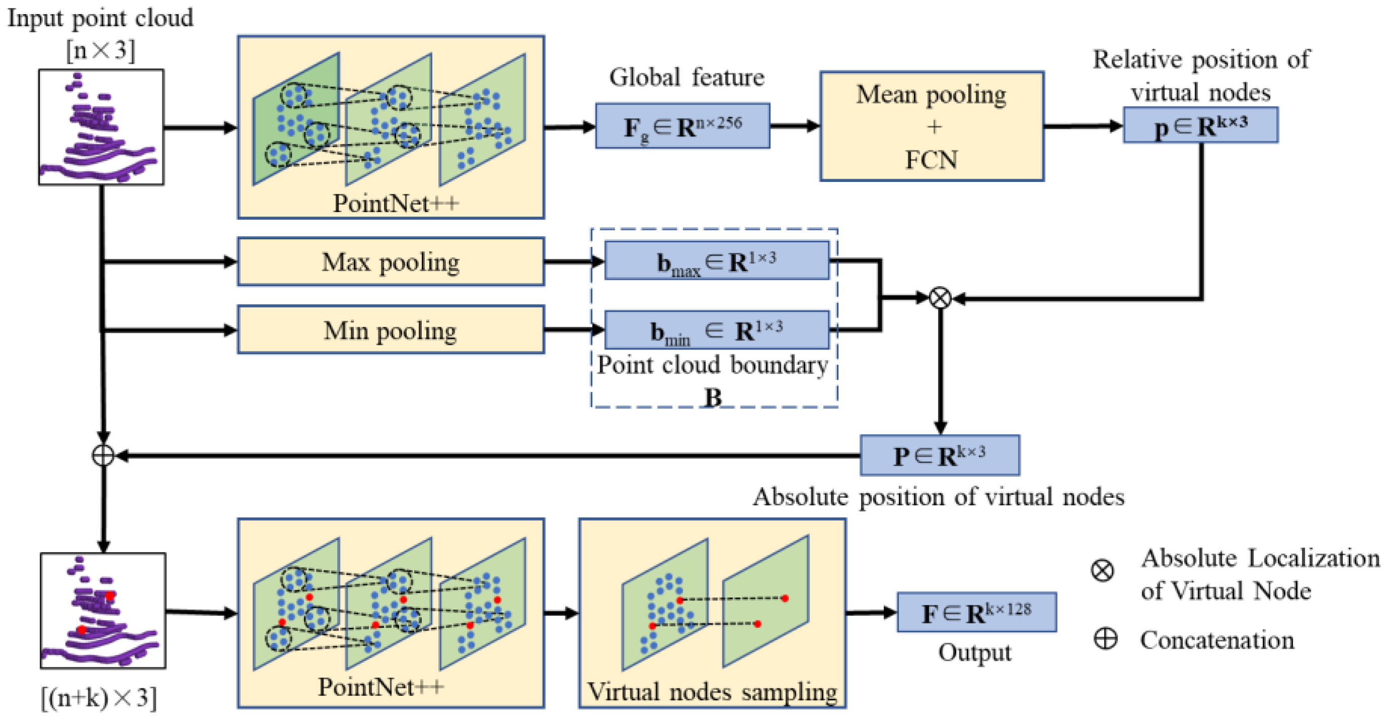
Figure 3. The feature extraction model based on movable virtual nodes.

3.3.1. Generation of Movable Virtual Nodes

The model takes the point cloud of templates or targets as input, with the number of points denoted as n. The centers of each input are aligned to the coordinate origin to reduce the impact of positional differences. Subsequently, global features (F_g) with dimensions (n × 256) are extracted from the input using the backbone of PointNet++. Additionally, the relative positions (p) of k virtual nodes within the overall point cloud are estimated through a combination of mean pooling and a fully connected network (FCN):

$$\mathbf{p}=\left[\begin{array}{c}\begin{array}{ccc}{x}_1& y_1& z_1\\ x_2& y_2& z_2\\ ⋮& ⋮& ⋮\\ x_{\mathrm{k}}& y_{\mathrm{k}}& z_{\mathrm{k}}\end{array}\end{array}\right],$$

(1)

(x_k, y_k, z_k) represents the relative position of the k-th virtual node within the input, with all values constrained within the range [0, 1]. Additionally, by applying max pooling and min pooling to the input point cloud, the vertices of the point cloud bounding box are represented as

$$\mathbf{B}=\left[\begin{array}{c}{\mathbf{b}}_{\max }\\ {\mathbf{b}}_{\min }\end{array}\right]=\left[\begin{array}{c}\begin{array}{ccc}{X}_{\max }& Y_{\max }& Z_{\max }\end{array}\\ \begin{array}{ccc}{X}_{\min }& Y_{\min }& Z_{\min }\end{array}\end{array}\right],$$

(2)

X_*, Y_*, Z_* represent the extremal values of the input point cloud in the three dimensions. The absolute position (P_k) of the virtual node can be determined as follows:

$${\mathbf{P}}_{\mathrm{k}}=\left[\begin{array}{ccc}{X}_{\mathrm{k}}& Y_{\mathrm{k}}& Z_{\mathrm{k}}\end{array}\right]={\mathbf{b}}_{\min }+\left[\begin{array}{ccc}{x}_{\mathrm{k}}& y_{\mathrm{k}}& z_{\mathrm{k}}\end{array}\right]\left[\begin{array}{ccc}{X}_{\max }-X_{\min }& 0& 0\\ 0& Y_{\max }-Y_{\min }& 0\\ 0& 0& Z_{\max }-Z_{\min }\end{array}\right],$$

(3)

3.3.2. Positioning of Movable Virtual Nodes

To effectively extract local information from focus regions, it is crucial to direct virtual nodes toward areas with significant local shape variations. To achieve this, we designed the VND metric, which measures the uniformity of point cloud distribution around virtual nodes and integrates it into the model’s loss function. During the training phase, adjustments are made to the model parameters to guide virtual nodes toward regions with significant shape variations, thereby enhancing localized features in these focus areas.

Specifically, we first define the range of the region where the k-th virtual node is located as L_k, referring to it as the Region of Interest (ROI).

$$L_{\mathrm{k}}=\left[\begin{array}{c}{l}_{\max }^{\mathrm{k}}\\ l_{\min }^{\mathrm{k}}\end{array}\right]=\left[\begin{array}{c}{P}_{\mathrm{k}}\\ P_{\mathrm{k}}\end{array}\right]+\left[\begin{array}{c}0.15\\ -0.15\end{array}\right]\left[b_{\max }-b_{\min }\right],$$

(4)

[b_max − b_min] is a 1 × 3 matrix. L_k is represented as a 2 × 3 matrix, where its elements denote the maximum and minimum values of the ROI across three dimensions. It is evident that the bounding box of the ROI is centered at the absolute position of the virtual node and proportionally scaled down from the input point cloud bounding box.

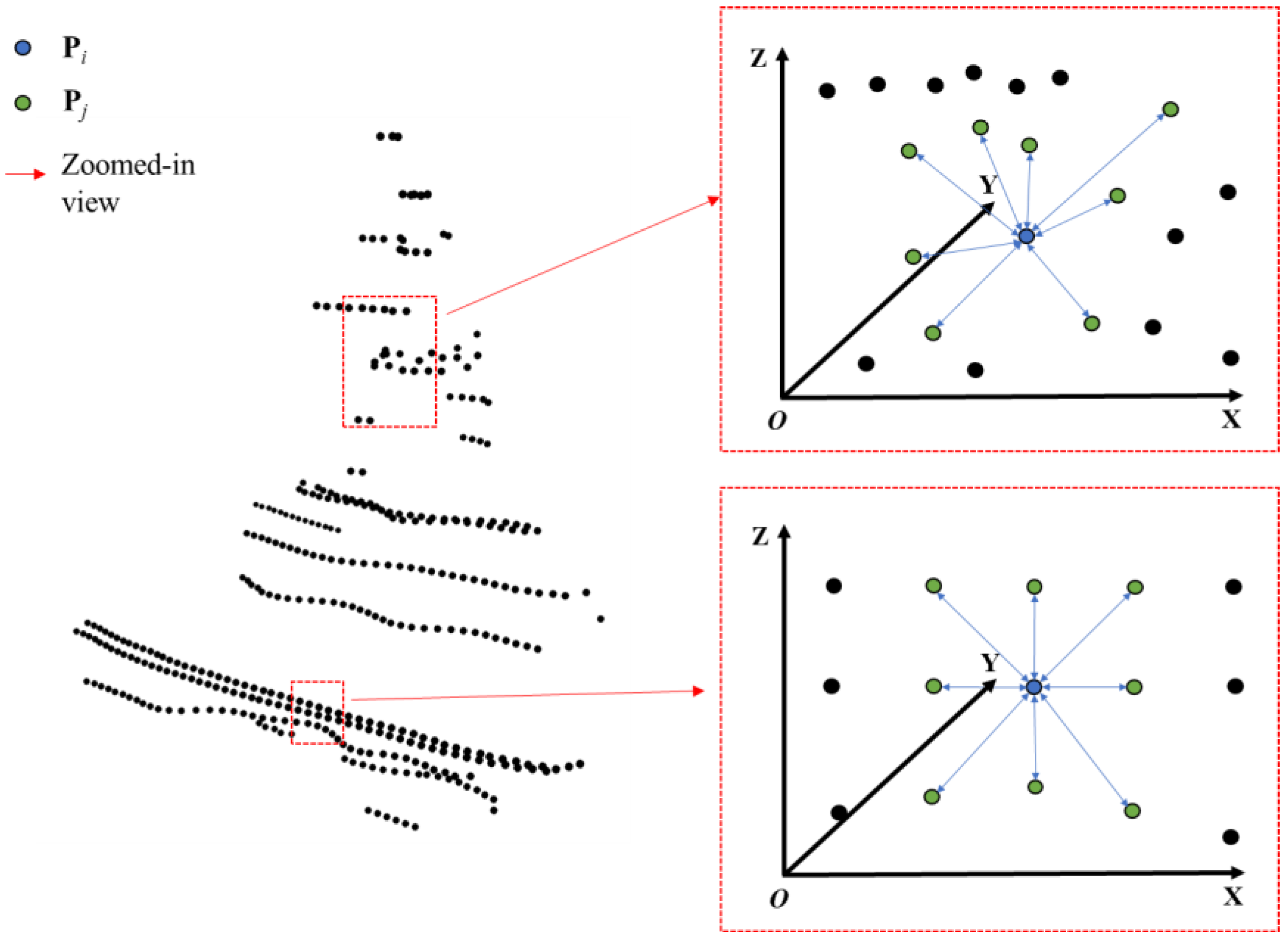
Furthermore, attention is focused on all points within the ROI. Inspired by the neighborhood range definition in image processing, an 8-nearest neighbor search is employed to determine the positions of the eight nearest points to each point, with the mean of these distances subsequently calculated.

$$d_i={\displaystyle \frac{1}{8}}{\displaystyle \sum _{j=1}^8\left(\sqrt{{\left(P_i-P_j\right)}^2}\right)}\hspace{1em}{P}_j\in N\left(P_i\right);i=1,2,\cdots ,m,$$

(5)

m denotes the number of point clouds within the ROI. P_i represents the coordinates of the i-th point within the ROI, P_j denotes the coordinates of the nearest neighbor point to P_i, and d_i represents the mean distance between P_i and its neighbor point. Finally, the variance of these mean distances is computed to obtain the VND.

$$\left\{\begin{array}{l}{V}_{\mathrm{k}}={\displaystyle \frac{1}{t}}{\displaystyle \sum _{i=1}^t{\left(d_i-d\right)}^2}\\ d={\displaystyle \frac{1}{t}}{\displaystyle \sum _{i=1}^t{d}_i}\end{array}\right.,$$

(6)

d denotes the mean of d_i within the ROI. V_k represents the VND of the k-th virtual node, which is the variance of these d_i values. This variance clearly indicates the uniformity of point cloud distribution within the ROI. As shown in Figure 4, regions with minor shape variations, such as the ship’s sides, exhibit uniform point cloud distribution, resulting in a small variance of d_i. In contrast, regions with significant shape variations, such as the mast, display non-uniform point cloud distribution, leading to a large variance of d_i.

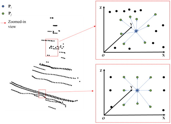
Figure 4. Illustration of point cloud distribution uniformity in different local areas of the USV.

When the ROI corresponds to a focus region with significant local shape variations, the point cloud distribution in that area tends to be more irregular, leading to an increased VND. By incorporating VND into the model’s loss function and maximizing it, the model is guided to accurately position the movable virtual nodes within the focus regions.

3.3.3. Virtual Point Sampling

We integrate the positions of virtual nodes into the original point cloud and employ the PointNet++ backbone to extract novel features from the updated point cloud. Furthermore, feature vectors (F) of the virtual nodes are sampled from the output of PointNet++. Leveraging the multilevel feature extraction and neighborhood aggregation capabilities of PointNet++, the network captures local information at various scales for each point. These local details are progressively integrated and updated across different layers to obtain more comprehensive global features. As a result, sampling the network’s output features at virtual nodes not only preserves the global characteristics of the input point cloud but also enhances the local information from the regions surrounding the virtual nodes.

3.4. Feature Matching

3.4.1. Revisiting Attention Module

The attention module was first applied to machine translation. Given input features G and H, the general formula for the attention module is:

$$\left\{\begin{array}{l}\mathbf{Q},\mathbf{K},\mathbf{V}=\mathrm{\alpha }\left(\mathbf{G}\right),\mathrm{\beta }\left(\mathbf{H}\right),\mathrm{\gamma }\left(\mathbf{H}\right)\\ \mathrm{\sigma }\left(\mathbf{Q},\mathbf{K}\right)=\mathbf{Q}·{\mathbf{K}}^T\\ \mathbf{\Omega }=\mathrm{\sigma }\left(\mathbf{Q},\mathbf{K}\right)\mathbf{V}\end{array}\right.,$$

(7)

where α, β and γ are point-wise feature transformations. Q, K, and V are the query, key and value matrices, respectively. The function σ is the relation function between Q and K, and is used to evaluate their similarity. When all elements of Q and K are independent random variables with zero mean and unit variance, the mean of their dot product is zero. As the correlation between Q and K increases, the dot product gradually increases. Ω is the attention feature produced by the attention module. It can be interpreted as the weighted sum of the column vectors of V, with weights given by σ (Q, K).

When G = H, the model as a self-attention mechanism, primarily capturing complex relationships within the input features to generate high-quality contextual representations. In this paper, it is used for aggregating features from multiple templates. When G and H are different inputs, the model as a cross-attention model, assessing the connections and differences between the input features. Here, it is used for similarity assessments between aggregated templates and targets.

3.4.2. Feature Matching Model with Double Attention

Due to technical limitations, a point cloud template typically comprises data captured from a single side of the USV. However, the point cloud of a cooperative USV in motion varies with its orientation. To identify and locate the cooperative USV among detected targets, we propose a feature matching model with double attention, termed DANet, which effectively identifies USVs with different orientations, even with limited templates.

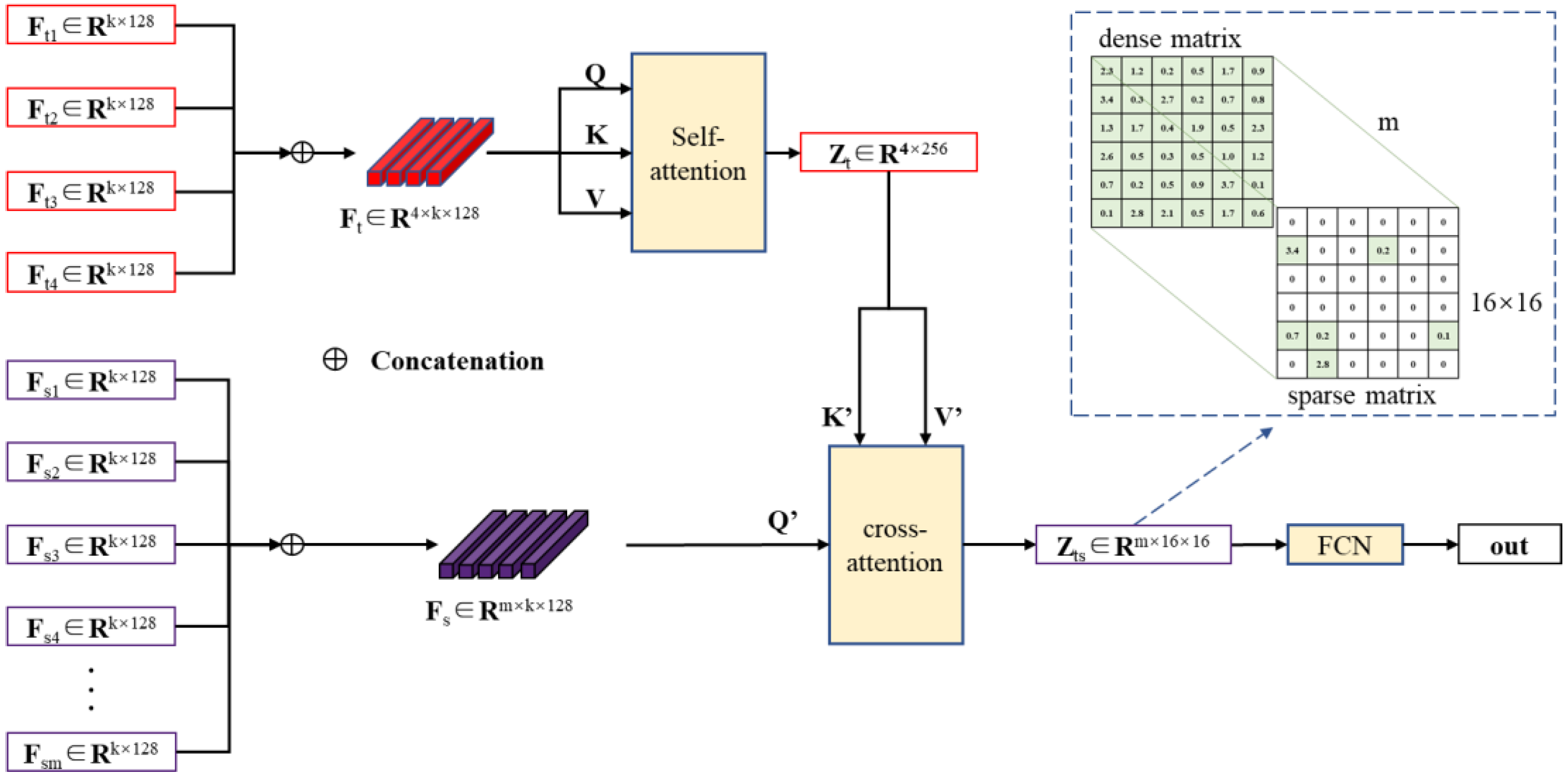
Initially, self-attention aggregates point cloud distribution features from the four templates, creating an aggregated feature for the external contour of the cooperative USV. Subsequently, cross-attention evaluates the similarity between the point cloud distribution features of targets and the aggregated template. This is then combined with a fully connected network to produce the final matching results. The workflow of the feature matching model is depicted in Figure 5.

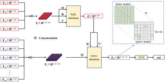
Figure 5. The feature matching model based on double attention.

In Figure 5, the point cloud distribution features extracted by MGNN from the four sides of the collaborative USV are concatenated and input into the self-attention network. Utilizing the Query (Q), Key (K), and Value (V) matrices, the self-attention network evaluates the similarity among the four templates and fuses information from different templates through weighted combinations. Specifically, Q represents the features of the current template, K represents the features of other templates, and the correlation degree between Q and K determines the similarity among the templates. V represents the actual feature representation. Based on equation (7), the weights of the templates are adjusted based on similarity scores, ultimately forming the fused representation Z_t.

Additionally, the point cloud distribution features of the target are concatenated and input into the cross-attention network. Unlike the self-attention network, the Key and Value matrices in the cross-attention network are derived from Z_t. The cross-attention network uses the similarity between the target feature and the aggregated template feature as weights to represent the target feature through a weighted combination of aggregated template features. As illustrated by Equation (7), when the target is not the collaborative USV, low similarity results in small weights, leading to sparsity in the target feature matrix generated by the weighted combination. In this paper, this results in a 16 × 16 sparse matrix. Conversely, when there is local similarity between the target and the templates (the target is a collaborative USV), larger weights are assigned, resulting in a denser target feature matrix. This generates a 16 × 16 dense matrix. The matrices generated by m targets ultimately compose an m × 16 × 16 output matrix Z_ts.

Using the relationship between target types and matrix sparsity, and in conjunction with the FCN, the final matching result is produced. The matching result is expressed in terms of probabilities, with the target having the highest probability being identified as the collaborative USV. In practical scenarios, the number of detected targets can vary. This paper sets the maximum number of targets in a single frame of data to eight. When the detected target count exceeds eight, only the eight targets closest to the USV are utilized. If the detected target count is less than 8, a masked softmax operation is applied to the excess input features, setting the feature matrix to a negligible value to deactivate the redundant input ports.

To train the model, we incorporate the deviation between the predicted matching results and the ground truth into the loss function. In this paper, we use cross-entropy to evaluate the matching performance.

$$J=-{\displaystyle \frac{1}{t}}{\displaystyle \sum _{i=1}^t\left[y_i\log \left(p_i\right)+\left(1-y_i\right)\log \left(1-p_i\right)\right]},$$

(8)

y_i denotes whether the i-th target is the collaborative USV, with 1 indicating a match and 0 indicating no match. p_i represents the matching probability of the i-th target as output by the model, and t stands for the number of targets. Since there are no learnable parameters in the subsequent rotating and clustering stage, we solely train the model parameters for feature extraction and feature matching. The overall loss function is defined as:

$$\mathrm{Loss}=\lambda J+{\displaystyle \frac{\mathrm{k}\left(1-\lambda \right)}{V_{\mathrm{k}}}},$$

(9)

λ is a hyperparameter, J represents the matching error, and V_k is VND of the region where the k-th virtual node is located.

3.5. Rotating and Clustering of Dual-View Point Cloud

To rectify the dual-view point cloud, we estimate the sway angles of the USV using the position of the collaborative USV as a reference. Specifically, after obtaining the point cloud of the collaborative USV through feature matching, we designate the point cloud center as the measured position of the collaborative USV. By combining this with the actual position provided by GNSS, we calculate the sway angles of the USV. These sway angles are then applied to correct the positions of the overall point clouds. Given the mutual collaborative relationship between the two USVs, this method can be used to rectify the point clouds acquired from both vessels.

In fact, the use of dual USVs can significantly increase the overall quantity of point clouds, and the corrected dual-view point clouds can position the obstacle point clouds in their true locations. Building on this, we use the DBSCAN algorithm to cluster the dual-view point clouds. This approach not only enables the extraction of obstacle positions but also, owing to the heightened quantity of point clouds in regions containing obstacles, effectively mitigates instances of missed detections.

4. Experiments

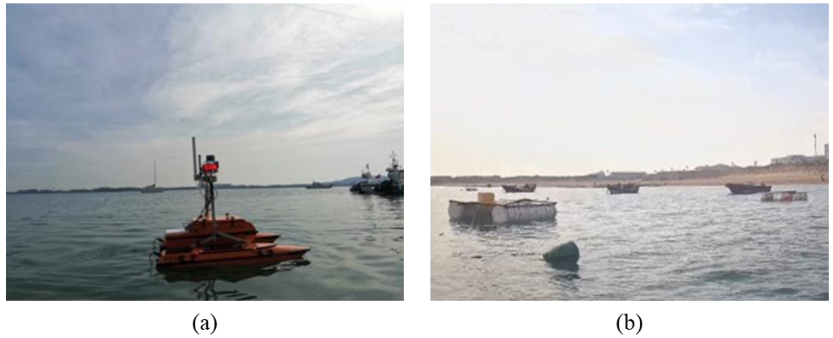
Given the current scarcity of practical dual-view point cloud datasets in ocean environments, we conducted multiple data collection sessions under level 1 and level 2 sea conditions in the Tangdaowan and Guzhenkou areas of Qingdao. Specifically, we gathered 8245 frames of data in Guzhenkou and 1125 frames in Tangdaowan. Each data frame includes dual-view point clouds, the USVs’ positions, and the count of detected obstacles. Figure 6 illustrates the experimental USV and some of the obstacles.

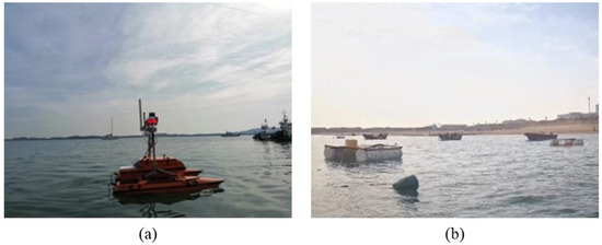
Figure 6. Experimental USV and some obstacles: (a) experimental USV; (b) obstacles.

Figure 6a shows the USV used in our experiments, while Figure 6b displays some of the marine obstacles. Additionally, we pre-collected point cloud data from all four sides of the USV as templates. The model underwent training and testing on an Intel(R) Xeon(R) Gold 6226R CPU @ 2.9 GHz and Nvidia Quadro RTX 6000 GPU. It’s important to note that all methods employed were fine-tuned by selecting optimal parameters to showcase their optimum performance.

4.1. Validation of the Feature Extraction Model

4.1.1. Experimental Protocol

(1)

Experimental data

This experiment uses 5771 frames of point cloud data from the Guzhenkou to train the model, with 2474 frames from Guzhenkou and 1125 frames from Tangdaowan used as validation sets to assess model performance.

(2)

Experimental setting

We evaluate feature extraction models with different numbers of virtual nodes (k = 0, 1, 2, 3, 4) to validate the necessity and effectiveness of MGNN. Notably, when k = 0, MGNN degenerates into the backbone of the traditional PointNet++, with virtual node sampling replaced by mean pooling and FCN. Since the output of the feature extraction model is not directly suitable for effectiveness evaluation, we integrate the feature matching model after the feature extraction model to assess its performance.

(3)

Evaluation metrics

We verify the model’s performance using precision, accuracy, and the mean value of VND (μ_v) during the testing phase. The calculation method for VND is provided in Equation (6), and the formulas for precision and accuracy are as follows:

$$\left\{\begin{array}{l}\mathrm{p}\mathrm{r}\mathrm{e}\mathrm{c}\mathrm{i}\mathrm{s}\mathrm{i}\mathrm{o}\mathrm{n}={\displaystyle \frac{TP}{TP+FP}}\\ \mathrm{a}\mathrm{c}\mathrm{c}\mathrm{u}\mathrm{r}\mathrm{a}\mathrm{c}\mathrm{y}={\displaystyle \frac{TP+TN}{TP+FN+TN+FP}}\end{array}\right.,$$

(10)

TP denotes the number of targets correctly identified as USVs, FN refers to the number of targets incorrectly identified as obstacles, TN represents the number of targets correctly identified as obstacles, and FP is the number of targets incorrectly identified as USVs. Since the model designed in this paper always selects the target with the highest similarity to the template as the collaborative USV, whenever the model mistakenly identifies a USV as an obstacle, an obstacle is inevitably identified as a USV, resulting in FN = FP. This means that recall is always equal to precision. Therefore, only precision is used as the evaluation metric in this paper.

4.1.2. Experimental Results and Analysis

Table 3 shows the model performance with different numbers of virtual nodes.

Table 3. Experimental results of the movable virtual nodes.

Model	Guzhenkou			Tangdaowan
	Precision	Accuracy	μV	Precision	Accuracy	μV
MGNN (k = 0) + DANet	0.8104	0.9271	\	0.7911	0.9197	\
MGNN (k = 1) + DANet	0.9038	0.9630	0.2679	0.8382	0.9378	0.3183
MGNN (k = 2) + DANet	0.9475	0.9798	0.2298	0.9147	0.9672	0.2630
MGNN (k = 3) + DANet	0.9345	0.9748	0.2175	0.9120	0.9662	0.2599
MGNN (k = 4) + DANet	0.9422	0.9778	0.1993	0.9013	0.9621	0.2542

Table 3 demonstrates that the incorporation of movable virtual nodes (k > 0) enhances both precision and accuracy compared to the model without movable virtual nodes (k = 0). The increase in precision confirms that virtual nodes effectively improve the model’s capability to identify USVs. Additionally, the rise in accuracy indicates that the model with virtual nodes performs better in identifying obstacles.

When k ≤ 2, as the number of virtual nodes increases, the precision and accuracy show a gradual increment. When k ≥ 2, the precision and accuracy stabilize. This trend can be attributed to the migration of redundant virtual nodes to the same position after the model training.

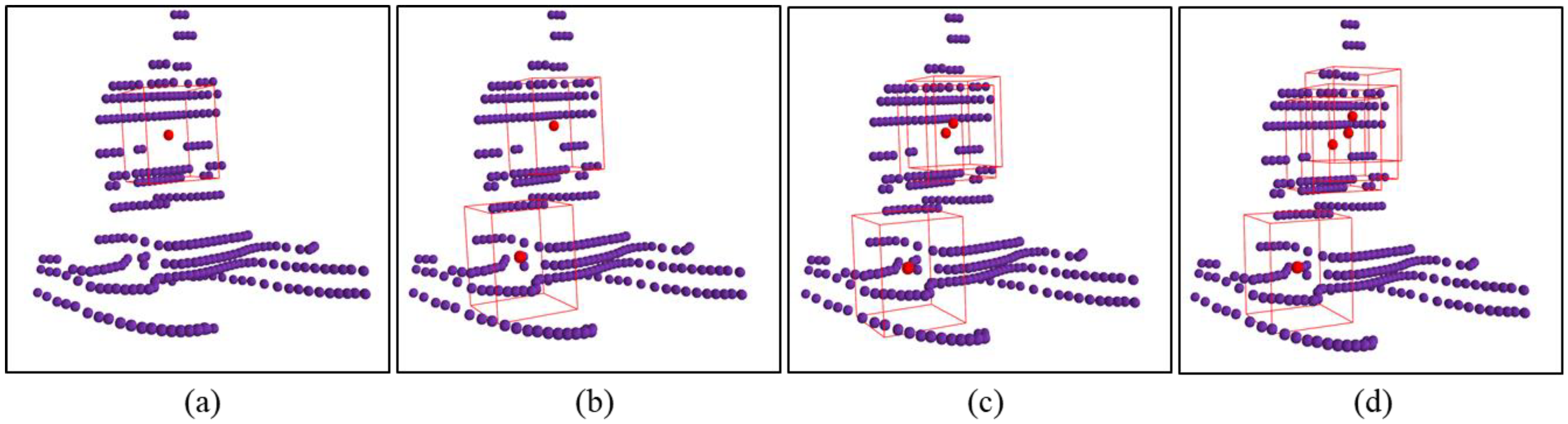
This trend is evident in the experimental data, where the decrease in mean VND slows with an increasing number of virtual nodes. To further illustrate this phenomenon, Figure 7 visualizes the positions of different numbers of virtual nodes on the collaborative USV’s point cloud. Note that, to enhance the clarity of the images, the point clouds in all the images in this paper have been dilated.

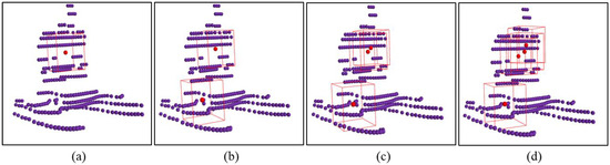
Figure 7. Visualization of the positions of virtual nodes in the point cloud of collaborative USV. (a) the number of virtual nodes is 1 (k = 1); (b) the number of virtual nodes is 2 (k = 2); (c) the number of virtual nodes is 3 (k = 3); (d) the number of virtual nodes is 4 (k = 4).

The fluctuation in μ_V indirectly suggests the occurrence of multiple virtual nodes converging to the same position. Specifically, when k = 1, virtual nodes are placed in the region with the maximum VND. With k = 2, guided by the matching error and VND in the loss function, the two virtual nodes point to distinct regions, resulting in a reduction in the mean VND. As k > 2, with no additional regions within the maritime target requiring special attention, the surplus virtual nodes aggregate towards the previously identified focus regions. This trend is evident in the experimental data, where the decrease in mean VND slows with an increasing number of virtual nodes. To further illustrate this phenomenon, Figure 7 visualizes the positions of different numbers of virtual nodes on the collaborative USV’s point cloud. Note that, to enhance the clarity of the images, the point clouds in all the images in this paper have been dilated.

Figure 7 illustrates the positions of virtual nodes generated by the feature extraction model for varying values of k. The purple points represent the point cloud of the collaborative USV, the red points indicate the positions of virtual nodes, and the red bounding box outlines the regions of interest. As shown in Figure 7, when 1 ≤ k ≤ 2, virtual nodes are dispersed across distinct regions. However, when k > 2, the newly introduced virtual nodes converge towards the same region. Evidently, the local features sampled by virtual nodes clustered in adjacent regions are similar, and this redundant information does not contribute to an increase in the precision and accuracy. Consequently, the precision and accuracy cease to grow with an increasing number of virtual nodes when k > 2.

In summary, we have validated the necessity and effectiveness of MGNN. Moreover, experimental results indicate that MGNN, with k = 2, demonstrates the highest adaptability in extracting features of maritime objects. Unless otherwise specified, MGNN (k = 2) will be employed as the feature extraction model in subsequent experiments.

4.2. Validation of Feature Matching

4.2.1. Experimental Protocol

(1)

Experimental data

The experimental data comprises all the point cloud data collected by the two USVs in the two sea areas. The division of the training and test sets follows the same scheme as described in Section 4.1.1. The USV templates and the point clouds of some typical objects used in the experiment are shown in Figure 8.

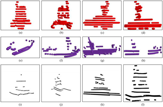
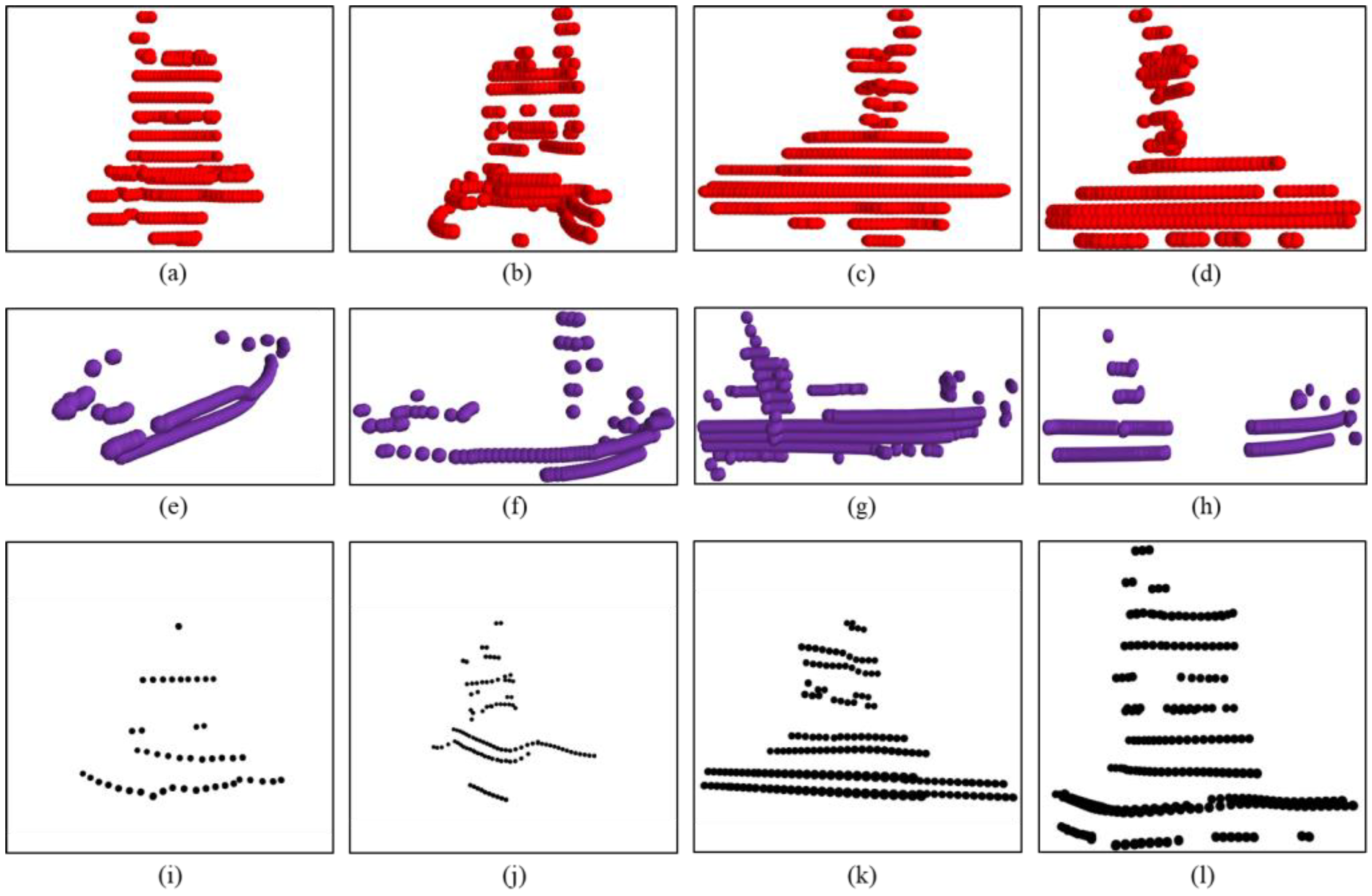
Figure 8. The USV templates and the captured point clouds of typical objects. (a–d) Templates of four different sides of the USV; (e–h) four typical maritime obstacles; (i–l) captured point cloud of the USV by another USV.

In Figure 8, the red point clouds in the first row represent USV templates, obtained from all four sides of the USV. The purple point clouds in the second row illustrate four typical maritime obstacles. The black point clouds in the third row represent a cooperative USV navigating in various orientations, as captured by another USV. These black point clouds contain 46, 109, 171, and 246 points, respectively. While there is a discernible global similarity between the USVs and the obstacles, significant differences exist in the point cloud distribution features of specific regions, such as masts and gunwales. Therefore, extracting the point cloud distribution features of focus regions is crucial for identifying USVs among the targets. Additionally, the variable orientations of the cooperative USV imply that its point clouds cannot consistently match a single template. Consequently, designing an aggregation model that integrates the point cloud distribution features from multiple templates holds considerable significance.

(2)

Experimental setting

To quantitatively assess the effectiveness of the proposed method, we integrated MGNN with DANet and conducted a comparative analysis with other state-of-the-art methods. The comparative methods include a manually designed feature-based template matching method, 3D-FM [27], and three deep learning methods (3D-SiamRPN [31], PTT-Net [32], and MCST-Net [35]). All comparative methods utilized the same template, with only one template employed per method.

Additionally, point clouds exhibit a characteristic of higher density in proximity and lower density at greater distances. As the distance between two vessels increases, the point cloud of the collaborative USV becomes increasingly sparse, raising the difficulty of template matching. Therefore, we divided the number of collaborative USV point clouds into four intervals and evaluated performance within each interval.

(3)

Evaluation metrics

The primary metrics for evaluation were precision, accuracy, and frames per second (FPS) in identifying collaborative USVs. It is essential to note that the proposed method predicts the target category, while some comparative methods predict the target’s position. To enable a direct comparison of performance, we consider a prediction as a correct identification of the collaborative USV if the predicted position center falls within the bounding box of the collaborative USV.

4.2.2. Experimental Results and Analysis

Table 4 presents the performance comparison of various methods on different datasets.

Table 4. The performance comparison of five methods.

Model		Guzhenkou				Tangdaowan
		n ≤ 50	50 < n ≤ 130	130 < n ≤ 200	n > 200	n ≤ 50	50 < n ≤ 130	130 < n ≤ 200	n > 200
3D-FM	precision	0.5213	0.6479	0.6604	0.6630	0.5281	0.6355	0.6446	0.6627
	accuracy	0.8026	0.8647	0.8695	0.8742	0.7593	0.8383	0.8451	0.8519
	FPS	15.9
3D-SiamRPN	precision	0.6064	0.7160	0.7166	0.7233	0.5393	0.6238	0.6355	0.6509
	accuracy	0.8378	0.8908	0.8911	0.8967	0.7605	0.8332	0.8411	0.8468
	FPS	23.8
PTT-Net	precision	0.6117	0.7071	0.7354	0.7452	0.5955	0.6939	0.7107	0.7278
	accuracy	0.8400	0.8874	0.8983	0.9049	0.7937	0.8642	0.8739	0.8805
	FPS	43.4
MCST-Net	precision	0.6383	0.7426	0.7442	0.7479	0.6067	0.7033	0.6993	0.7101
	accuracy	0.8509	0.9011	0.9017	0.9059	0.7994	0.8684	0.8689	0.8727
	FPS	35.7
Ours	precision	0.8085	0.9497	0.9647	0.9698	0.7753	0.9159	0.9339	0.9349
	accuracy	0.9211	0.9807	0.9864	0.9888	0.8854	0.9627	0.9712	0.9714
	FPS	38.2

In Table 4, n represents the number of collaborative USV point clouds, which is primarily related to the distance between the two vessels. n = 50 corresponds to approximately 40 m between the two USVs. As shown in Figure 8, when n < 50, the USV point cloud becomes exceedingly sparse.

Our proposed method outperforms all other comparative methods across all intervals. Specifically, the average performance of our method exceeds that of 3D-FM, 3D-SiamRPN, PTT-Net, and MCST-Net by approximately 29%, 26%, 22%, and 20% in precision, respectively. In terms of accuracy, the average performance of our method surpasses 3D-FM, 3D-SiamRPN, PTT-Net, and MCST-Net by about 12%, 11%, 9%, and 8%, respectively. This improvement is primarily due to our method using point clouds from four different sides of the collaborative USV as templates, allowing for accurate matching regardless of the USV’s orientation. To better illustrate the superiority of our method, Figure 9 presents a scatter plot comparing the precision and accuracy of various methods.

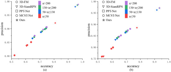
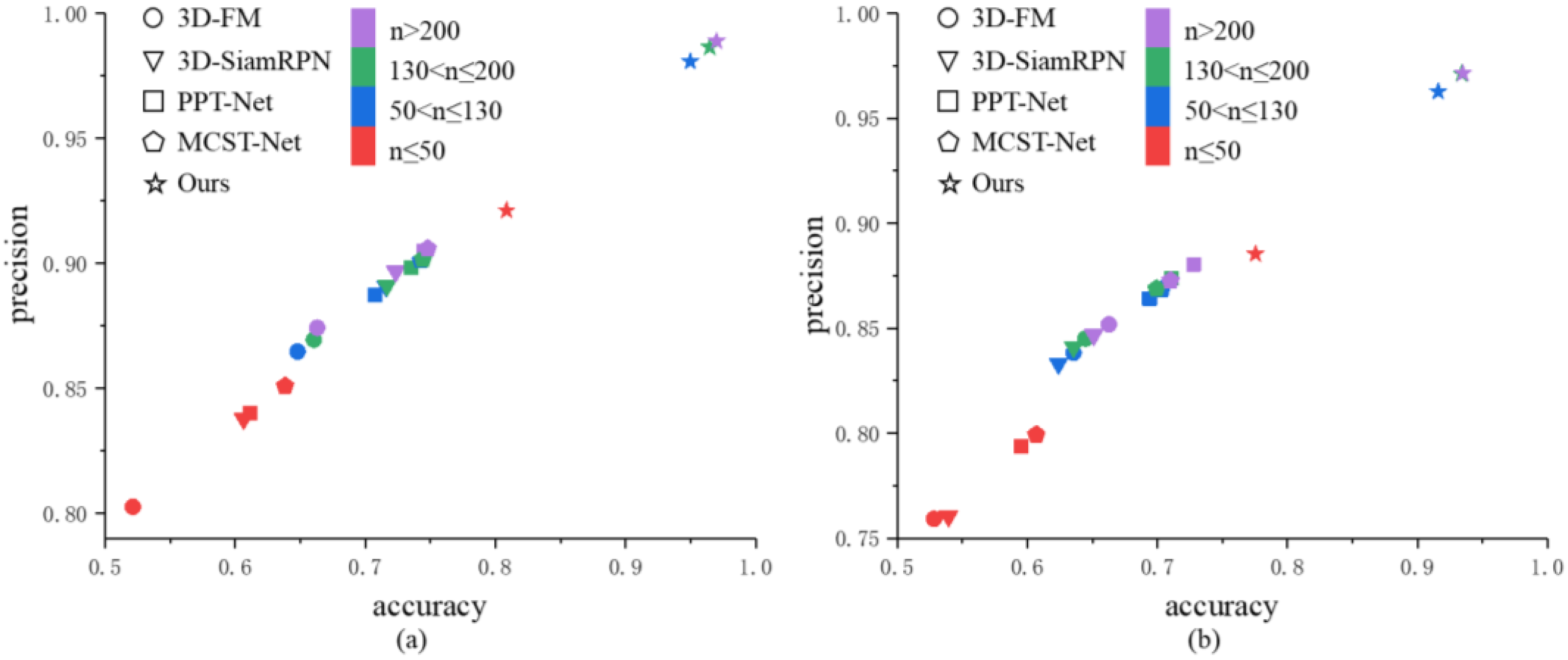
Figure 9. Accuracy vs. precision in four intervals of the point cloud quantity. (a) Guzhenkou datasets; (b) Tangdaowan datasets.

As shown in Figure 9, our proposed method achieves state-of-the-art performance in both precision and accuracy. Notably, when the point cloud quantity for the collaborative USVs remains above 50, which corresponds to a distance of less than 40 m between the two vessels, our method is relatively insensitive to reductions in point cloud quantity. In contrast, the performance of comparative methods declines significantly. Even when the point cloud quantity falls below 50, although our method experiences a slight decrease in performance, it still outperforms all comparative methods.

We attribute the performance decline of comparative methods in sparse point clouds to the loss of local features. This issue is particularly evident in traditional methods like 3D-FM, which rely heavily on the complete consistency between the target and template point clouds. As the point cloud becomes sparser, the spatial relationships between neighboring points are altered significantly, leading to changes in point cloud distribution features and, consequently, affecting matching performance. The deterioration in matching performance due to the loss of local features highlights the crucial role of local features in template matching, reinforcing the necessity of extracting local features from focus regions. Overall, our method demonstrates strong robustness in extremely sparse scenarios.

In terms of time efficiency, considering that the actual sailing speed of USV is only 1–2 m/s, the speed requirement for obstacle detection is relatively low (FPS > 3). Thus, the proposed method meets the real-time requirements for USV obstacle detection. Comparatively, our method significantly outperforms the traditional feature matching method 3D-FM, with an increase of 22.3 FPS. This is because 3D-FM is fundamentally an optimization algorithm, which, compared to end-to-end deep learning methods, has lower computational efficiency. Among deep learning methods, our method outperforms 3D-SiamRPN and MCST-Net by 37% and 7%, respectively. This improvement can be attributed to the attention mechanism used in both our method and MCST-Net, which allows for parallel processing of data and significantly reduces processing time. Additionally, our method’s slight advantage over MCST-Net can be attributed to its lighter network architecture and fewer parameters. However, our method’s real-time performance is somewhat inferior to PTT-Net, which uses a specifically designed efficient point cloud processing method to enhance computation speed by sampling input point clouds to reduce model input dimensions. Nevertheless, this sampling inevitably results in the loss of some local feature information, affecting the final matching results.

To further validate the scalability of the proposed method with different USV configurations, we ran the proposed method on an Intel(R) Core(TM) i5-7300HQ CPU, achieving an FPS of 6.6, which still meets practical use requirements. In the future, optimizing the point cloud sampling process to minimize information loss in focus regions could help improve computation speed while maintaining precision and accuracy.

Comparing the experimental results across different maritime areas, the consistent performance of the same method in various regions suggests the reliability of the experimental environments and settings. Notably, the proposed method exhibits excellent performance in both the Guzhenkou and Tangdaowan areas, affirming its adaptability to diverse environments. This robust performance lends strong support to the reliability of our method in practical applications.

4.3. Validation of Obstacle Detection for Dual USVs

4.3.1. Experimental Protocol

(1)

Experimental data

We conducted obstacle detection experiments utilizing 761 frames of dual-view point cloud data obtained at Guzhenkou. The experimental scenarios encompassed obstacles such as plastic rafts and fishing boats.

(2)

Experimental setting

To validate the effectiveness of dual USVs in improving obstacle detection, we employed several obstacle detection methods on a single USV as benchmarks. The comparative methods include the Euclidean Clustering with Adaptive Neighborhood Radius (ECANR) method [36], the KD-Tree Enhanced Euclidean Clustering (KDEC) method [37,38], the Grid Clustering (GC) method [9], and the Point Distance-Based Segmentation (PDBS) method [10].

Similar to our method, the comparative methods are all based on clustering algorithms for obstacle detection. Among them, the GC algorithm is a traditional lidar-based method that clusters obstacles using an occupancy grid. To address the characteristic of point clouds being dense near the sensor and sparse further away, the ECANR algorithm dynamically adjusts clustering thresholds based on the distance between the grid and the USV to improve detection performance. In contrast, the KDEC and PDBS algorithms directly process point clouds, with KDEC clustering based on distances between points and PDBS clustering based on angular differences between the point clouds and the observer.

(3)

Evaluation metrics

Building upon the experiments, we conducted both qualitative and quantitative analyses to evaluate the effectiveness of the proposed dual USV obstacle detection method. For the quantitative analysis, we used the missed detection rate and the false alarm rate of obstacles as evaluation metrics.

$$\left\{\begin{array}{c}{R}_m={\displaystyle \frac{F{N}^{\prime }}{T{P}^{\prime }+F{N}^{\prime }}}\\ R_f={\displaystyle \frac{F{P}^{\prime }}{T{P}^{\prime }+F{P}^{\prime }}}\end{array}\right.,$$

(11)

R_m represents the missed detection rate, and R_f denotes the false alarm rate. TP’ refers to the number of detected obstacles, FN’ is the number of undetected obstacles, and FP’ signifies the number of targets incorrectly identified as obstacles.

4.3.2. Qualitative Analysis

The qualitative analysis compares the detection results between single USV and dual USVs in a typical scene, as depicted in Figure 10.

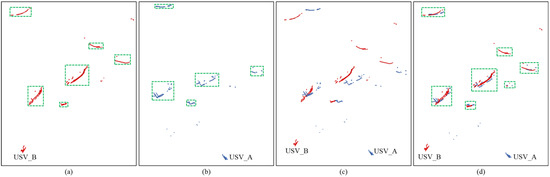
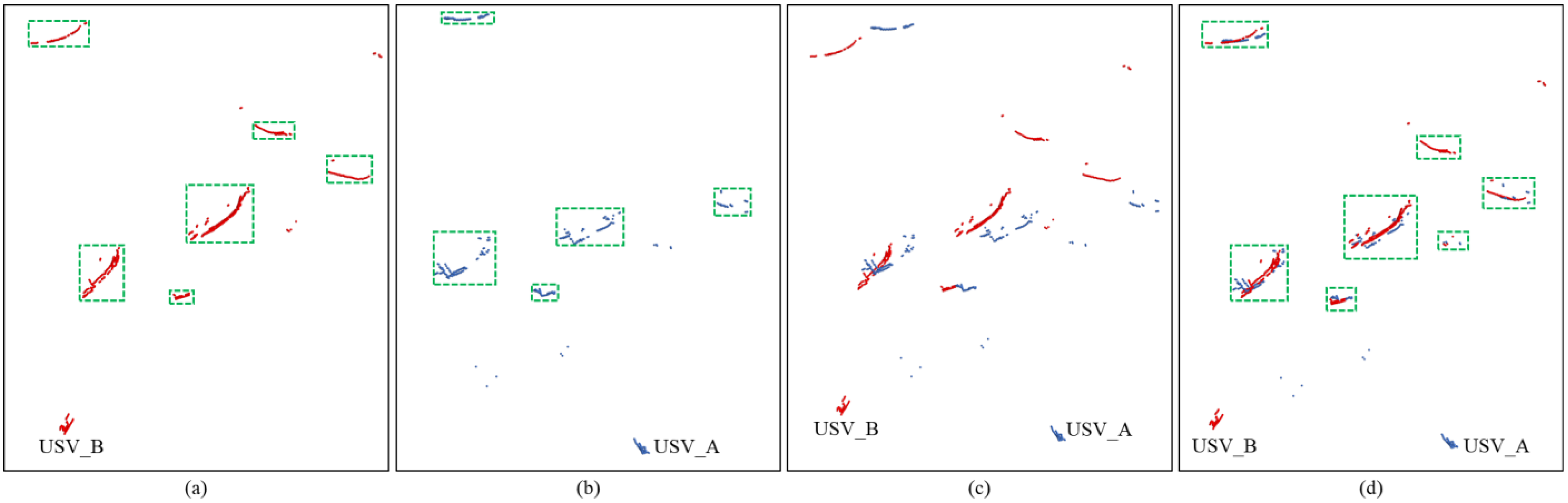
Figure 10. The visual comparison between the results of single USV detection and dual USV detection in a typical scene. (a) the detection result of the USV_A at the bottom right; (b) the detection result of the USV_B at the bottom left; (c) the dual-view point clouds before rotational correction; (d) the corrected dual-view point cloud and detection result.

In Figure 10, the blue and red points represent the point clouds collected by two USVs. The USVs are positioned at the bottom left and bottom right of the figure, with their locations marked in the point clouds collected by each other. The point clouds in the three images are labeled with obstacle positions using the DBSCAN algorithm with consistent parameter settings, and the green boxes highlight the detected obstacles. Specifically, Figure 10a shows the point cloud collected by USV_A located at the bottom right, while Figure 10b presents the point cloud from USV_B at the bottom left. It is important to note that, to mitigate interference from waves generated during navigation, the LiDAR typically filters out point clouds around itself, hence, the visualized images do not show the observer’s own point clouds. Figure 10c depicts the point cloud from both USVs before rotation, and Figure 10d illustrates the dual-view point cloud after positional correction.

To effectively demonstrate the superiority of the proposed method, we conducted a comparison of detection results. Upon comparing Figure 10a with Figure 10d, it is evident that a small target was missed in Figure 10a. This occurred because the point cloud of this small target in Figure 10a had fewer points, leading the clustering method to consider it as noise generated by waves and filter it out. Furthermore, comparing Figure 10b with Figure 10d, it becomes apparent that not only was a small target missed in Figure 10b, but an occluded target was also missed. However, these instances of missed detection were effectively addressed in the dual USVs detection scenario depicted in Figure 10d. This improvement can be attributed to the complementary information provided by the dual-view point cloud and the correction of point cloud positions. Figure 10c clearly demonstrates the importance of positional correction. In Figure 10c, due to the absence of positional correction, the point clouds belonging to the same target deviate from their true positions. With positional correction, as shown in Figure 10d, the obstacles’ point clouds captured by the dual USVs are effectively aligned with the regions where the obstacles were located. On the one hand, the dual-view point cloud, acquired from different perspectives, effectively mitigated the issue of missed detections caused by occlusion. On the other hand, the increased number of points within the target areas enabled the clustering method to effectively detect small targets.

4.3.3. Quantitative Analysis

Table 5 presents the missed detection rate and false alarm rate of various methods.

Table 5. Comparison of obstacle detection performance.

Method	Miss Detection Rate	False Alarm Rate
ours	0.0615	0.0294
ECANR	0.1745	0.0215
KDEC	0.1514	0.0256
GC	0.2084	0.0183
PDBS	0.1403	0.0247

From Table 5, it is evident that utilizing dual USVs significantly improves obstacle detection. Compared to single USV obstacle detection results, the proposed method reduces the missed detection rate by 7.88% to 14.69%. The reduction in missed detections can be attributed to the increased quantity of point clouds for obstacles. When using a single LiDAR, the point cloud data for small obstacles, such as buoys and plastic rafts, or obstructed obstacles, is often limited. Clusters formed by a small number of points are frequently misidentified as interference and subsequently filtered out, leading to missed detections. In contrast, the proposed method effectively utilizes point clouds from different perspectives provided by the two USVs. By correcting the dual-view point clouds to increase the number of points in the region where obstacles are located, the proposed method enhances the contrast between obstacles and interference, thereby reducing missed detections.

However, compared to other methods, the proposed method shows a slight increase in false alarms caused by sea waves. Specifically, while the correction of dual-view point clouds increases the number of points in obstacle regions, it also increases the point quantity in areas where sea waves are detected by both USVs simultaneously. This additional point cloud in wave regions can lead to false positives. In practice, the occurrence of both USVs detecting the same sea wave is rare due to the stringent conditions required—namely, the relative position of the waves to the two USVs and the height of the waves must meet specific criteria. In our experiments, this resulted in only a slight increase in the false alarm rate, ranging from 0.38% to 1.11%.

5. Conclusions

This paper proposes an obstacle detection method for dual USVs based on movable virtual nodes and double attention. The method rectifies dual-view point clouds using the two USVs as mutual references, thereby augmenting the point cloud quantity within regions where maritime obstacles are located. The amplified quantity of point clouds enhances the differentiation between obstacles and interference, consequently improving the obstacle detection. The primary focus of the proposed method is to employ template matching for the identification of the collaborative USV among the detected targets.

In the process of template matching, we designed a feature extraction model based on movable virtual nodes. This model realizes feature extraction while enhancing the point cloud distribution features of the focus regions. Additionally, we proposed a feature matching model based on double attention, which aggregates the point cloud distribution features of templates from all four sides of the collaborative USV and identifies the collaborative USV based on the similarity between the target and the aggregated template. Our method has been validated on a self-collected dataset, demonstrating substantial advantages over existing mainstream methods.

It is crucial to emphasize that the proposed method is susceptible to shore interference. In areas near the coastline, where numerous terrestrial objects are present, the abundance of items may pose a substantial challenge to template matching, potentially impeding the effectiveness of obstacle detection. To address these issues, the following methods can be employed:

• Utilize high-precision map information to filter out point clouds from coastal areas.
• Implement an adaptive threshold mechanism that adjusts the sensitivity of template matching based on the distance to the coastline.
• Develop a point cloud registration method based on the overall coastline profile, aligning dual-view coastlines to correct point cloud positions.
• Integrate data from multiple sensors, such as LiDAR and cameras, to leverage their respective advantages and enhance the resilience of template matching against interference.

References

- Xiong, Y.; Zhu, H.; Pan, L.; Wang, J. Research on intelligent trajectory control method of water quality testing unmanned surface vessel. J. Mar. Sci. Eng. 2022, 10, 1252. [Google Scholar] [CrossRef]
- Ang, Y.; Ng, W.; Chong, Y.; Wan, J.; Chee, S.; Firth, L. An autonomous sailboat for environment monitoring. In Proceedings of the 2022 Thirteenth International Conference on Ubiquitous and Future Networks, Barcelona, Spain, 5–8 July 2022. [Google Scholar]
- Smith, T.; Mukhopadhyay, S.; Murphy, R.; Manzini, T.; Rodriguez, I. Path coverage optimization for USV with side scan sonar for victim recovery. In Proceedings of the 2022 IEEE International Symposium on Safety, Security, and Rescue Robotics, Sevilla, Spain, 8–10 November 2022. [Google Scholar]
- Kim, E.; Nam, S.; Ahn, C.; Lee, S.; Koo, J.; Hwang, T. Comparison of spatial interpolation methods for distribution map an unmanned surface vehicle data for chlorophyll-a monitoring in the stream. Environ. Technol. Innov. 2022, 28, 102637. [Google Scholar] [CrossRef]
- Cheng, L.; Deng, B.; Yang, Y.; Lyu, J.; Zhao, J.; Zhou, K.; Yang, C.; Wang, L.; Yang, S.; He, Y. Water target recognition method and application for unmanned surface vessels. IEEE Access 2022, 10, 421–434. [Google Scholar] [CrossRef]
- Sun, X.; Liu, T.; Yu, X.; Pang, B. Unmanned surface vessel visual object detection under all-weather conditions with optimized feature fusion network in YOLOv4. J. Intell. Robot. Syst. 2021, 103, 55. [Google Scholar] [CrossRef]
- Yang, Z.; Li, Y.; Wang, B.; Ding, S.; Jiang, P. A lightweight sea surface object detection network for unmanned surface vehicles. J. Mar. Sci. Eng. 2022, 10, 965. [Google Scholar] [CrossRef]
- Xie, B.; Yang, Z.; Yang, L.; Wei, A.; Weng, X.; Li, B. AMMF: Attention-based multi-phase multi-task fusion for small contour object 3D detection. IEEE Trans. Intell. Transp. Syst. 2023, 24, 1692–1701. [Google Scholar] [CrossRef]
- Gonzalez-Garcia, A.; Collado-Gonzalez, I.; Cuan-Urquizo, R.; Sotelo, C.; Sotelo, D.; Castañeda, H. Path-following and LiDAR-based obstacle avoidance via NMPC for an autonomous surface vehicle. Ocean Eng. 2022, 266, 112900. [Google Scholar] [CrossRef]
- Han, J.; Cho, Y.; Kim, J.; Kim, J.; Son, N.; Kim, S. Autonomous collision detection and avoidance for ARAGON USV Development and field tests. J. F. Robot. 2020, 37, 987–1002. [Google Scholar] [CrossRef]
- Sun, J.; Ji, Y.; Wu, F.; Zhang, C.; Sun, Y. Semantic-aware 3D-voxel CenterNet for point cloud object detection. Comput. Electr. Eng. 2022, 98, 107677. [Google Scholar] [CrossRef]
- He, Z.; Dai, Y.; Li, L.; Xu, H.; Jin, J.; Liu, D. A coastal obstacle detection framework of dual USVs based on dual-view color fusion. Signal Image Video Process. 2023, 17, 3883–3892. [Google Scholar] [CrossRef]
- Peng, Z.; Liu, E.; Pan, C.; Wang, H.; Wang, D.; Liu, L. Model-based deep reinforcement learning for data-driven motion control of an under-actuated unmanned surface vehicle: Path following and trajectory tracking. J. Frankl. Inst.-Eng. Appl. Math. 2023, 360, 4399–4426. [Google Scholar] [CrossRef]
- Wu, B.; Yang, L.; Wu, Q.; Zhao, Y.; Pan, Z.; Xiao, T.; Zhang, J.; Wu, J.; Yu, B. A stepwise minimum spanning tree matching method for registering vehicle-borne and backpack LiDAR point clouds. IEEE Trans. Geosci. Remote Sens. 2022, 60, 5705713. [Google Scholar] [CrossRef]
- Wang, F.; Hu, H.; Ge, X.; Xu, B.; Zhong, R.; Ding, Y.; Xie, X.; Zhu, Q. Multientity registration of point clouds for dynamic objects on complex floating platform using object silhouettes. IEEE Trans. Geosci. Remote Sens. 2021, 59, 769–783. [Google Scholar] [CrossRef]
- Yue, X.; Liu, Z.; Zhu, J.; Gao, X.; Yang, B.; Tian, Y. Coarse-fine point cloud registration based on local point-pair features and the iterative closest point algorithm. Appl. Intell. 2022, 52, 12569–12583. [Google Scholar] [CrossRef]
- Gu, B.; Liu, J.; Xiong, H.; Li, T.; Pan, Y. ECPC-ICP: A 6D vehicle pose estimation method by fusing the roadside lidar point cloud and road feature. Sensors 2021, 21, 3489. [Google Scholar] [CrossRef]
- He, Y.; Yang, J.; Xiao, K.; Sun, C.; Chen, J. Pose tracking of spacecraft based on point cloud DCA features. IEEE Sens. J. 2022, 22, 5834–5843. [Google Scholar] [CrossRef]
- Yang, Y.; Fang, G.; Miao, Z.; Xie, Y. Indoor-outdoor point cloud alignment using semantic-geometric descriptor. Remote Sens. 2022, 14, 5119. [Google Scholar] [CrossRef]
- Zhang, Z.; Zheng, J.; Tao, Y.; Xiao, Y.; Yu, S.; Asiri, S.; Li, J.; Li, T. Traffic sign based point cloud data registration with roadside LiDARs in complex traffic environments. Electronics 2022, 11, 1559. [Google Scholar] [CrossRef]
- Naus, K.; Marchel, L. Use of a weighted icp algorithm to precisely determine USV movement parameters. Appl. Sci. -Basel 2019, 9, 3530. [Google Scholar] [CrossRef]
- Xie, L.; Zhu, Y.; Yin, M.; Wang, Z.; Ou, D.; Zheng, H.; Liu, H.; Yin, G. Self-feature-based point cloud registration method with a novel convolutional siamese point net for optical measurement of blade profile. Mech. Syst. Signal Process. 2022, 178, 109243. [Google Scholar] [CrossRef]
- Sun, L.; Zhang, Z.; Zhong, R.; Chen, D.; Zhang, L.; Zhu, L.; Wang, Q.; Wang, G.; Zou, J.; Wang, Y. A weakly supervised graph deep learning framework for point cloud registration. IEEE Trans. Geosci. Remote Sens. 2022, 60, 5702012. [Google Scholar] [CrossRef]
- Yi, R.; Li, J.; Luo, L.; Zhang, Y.; Gao, X.; Guo, J. DOPNet: Achieving accurate and efficient point cloud registration based on deep learning and multi-level features. Sensors 2022, 22, 8217. [Google Scholar] [CrossRef] [PubMed]
- Ding, J.; Chen, H.; Zhou, J.; Wu, D.; Chen, X.; Wang, L. Point cloud objective recognition method combining SHOT features and ESF features. In Proceedings of the 12th International Conference on Cyber-Enabled Distributed Computing and Knowledge Discovery, Xi’an, China, 15–16 December 2022. [Google Scholar]
- Guo, Z.; Mao, Y.; Zhou, W.; Wang, M.; Li, H. CMT: Context-matching-guided transformer for 3D tracking in point clouds. In Proceedings of the 17th European Conference on Computer Vision, Tel Aviv, Israel, 23–27 October 2022. [Google Scholar]
- Yu, Y.; Guan, H.; Li, D.; Jin, S.; Chen, T.; Wang, C.; Li, J. 3-D feature matching for point cloud object extraction. IEEE Geosci. Remote Sens. Lett. 2020, 17, 322–326. [Google Scholar] [CrossRef]
- Gao, H.; Geng, G. Classification of 3D terracotta warrior fragments based on deep learning and template guidance. IEEE Access 2020, 8, 4086–4098. [Google Scholar] [CrossRef]
- Giancola, S.; Zarzar, J.; Ghanem, B. Leveraging shape completion for 3D siamese tracking. In Proceedings of the 32nd IEEE/CVF Conference on Computer Vision and Pattern Recognition, Long Beach, CA, USA, 16–20 June 2019. [Google Scholar]
- Qi, H.; Feng, C.; Cao, Z.; Zhao, F.; Xiao, Y. P2B: Point-to-box network for 3D object tracking in point clouds. In Proceedings of the IEEE/CVF Conference on Computer Vision and Pattern Recognition, Seattle, WA, USA, 14–19 June 2020. [Google Scholar]
- Fang, Z.; Zhou, S.; Cui, Y.; Scherer, S. 3D-SiamRPN: An end-to-end learning method for real-time 3d single object tracking using raw point cloud. IEEE Sens. J. 2021, 21, 4995–5011. [Google Scholar] [CrossRef]
- Shan, J.; Zhou, S.; Cui, Y.; Fang, Z. Real-Time 3D single object tracking with transformer. IEEE Trans. Multimed. 2023, 25, 2339–2353. [Google Scholar] [CrossRef]
- Zhou, C.; Luo, Z.; Luo, Y.; Liu, T.; Pan, L.; Cai, Z.; Zhao, H.; Lu, S. PTTR: Relational 3d point cloud object tracking with transformer. In Proceedings of the IEEE Conference on Computer Vision and Pattern Recognition, New Orleans, LA, USA, 18–24 June 2022. [Google Scholar]
- Hui, H.; Wang, L.; Tang, L.; Lan, K.; Xie, J.; Yang, J. 3D siamese transformer network for single object tracking on point clouds. In Proceedings of the 17th European Conference on Computer Vision, Tel Aviv, Israel, 23–27 October 2022. [Google Scholar]
- Feng, S.; Liang, P.; Gao, J.; Cheng, E. Multi-correlation siamese transformer network with dense connection for 3D single object tracking. IEEE Robot. Autom. Lett. 2023, 8, 8066–8073. [Google Scholar] [CrossRef]
- Lin, J.; Koch, L.; Kurowski, M.; Gehrt, J.; Abel, D.; Zweigel, R. Environment perception and object tracking for autonomous vehicles in a harbor scenario. In Proceedings of the 23rd IEEE International Conference on Intelligent Transportation Systems, Electr network, Rhodes, Greece, 20–23 September 2020. [Google Scholar]
- Liu, C.; Xiang, X.; Huang, J.; Yang, S.; Shaoze, Z.; Su, X.; Zhang, Y. Development of USV autonomy: Architecture, implementation and sea trials. Brodogradnja 2022, 73, 89–107. [Google Scholar] [CrossRef]
- Zhang, W.; Jiang, F.; Yang, C.; Wang, Z.; Zhao, T. Research on unmanned surface vehicles environment perception based on the fusion of vision and lidar. IEEE Access 2021, 9, 63107–63121. [Google Scholar] [CrossRef]
Disclaimer/Publisher’s Note: The statements, opinions and data contained in all publications are solely those of the individual author(s) and contributor(s) and not of MDPI and/or the editor(s). MDPI and/or the editor(s) disclaim responsibility for any injury to people or property resulting from any ideas, methods, instructions or products referred to in the content. |
© 2024 by the authors. Licensee MDPI, Basel, Switzerland. This article is an open access article distributed under the terms and conditions of the Creative Commons Attribution (CC BY) license (https://creativecommons.org/licenses/by/4.0/).