Optimization-Assisted Filter for Flow Angle Estimation of SUAV Without Adequate Measurement

Abstract

The accurate estimation of flow angles is crucial for enhancing flight performance and aircraft safety. Flow angles of fixed-wing small unmanned aerial vehicles (SUAVs) are more vulnerable due to their low airspeed. Current flow angle measurement devices have not been widely implemented in SUAVs due to their substantial cost and size constraints. Moreover, there are no general estimation methods suitable for SUAVs based on their rudimentary sensor suite. This study presents a generalized optimization-assisted filter estimation (OAFE) method for estimating the relative velocity and flow angles of fixed-wing SUAVs based on a standard sensor suite. This OAFE method mainly consists of a cubature Kalman filter and an optimizer. The filter serves as the main loop with which to generate flow angles in real time by fusing the acceleration, angular rate, attitude, and airspeed. Without flow angle measurements, the optimizer generates approximate aerodynamic derivatives, which serve as pseudo-measurements with which to refine the performance of the filter. The results demonstrate that the estimated angle of attack and side slip angle displayed root mean square errors of around 0.11° and 0.24° in the simulation. The feasibility was also verified in field tests. The OAFE method does not require flow angle measurements, the prior acquisition of aerodynamic parameters, or model training, making it suitable for quick deployment on different SUAVs.

1. Introduction

In recent years, fixed-wing small unmanned aerial vehicles (SUAVs) have evolved rapidly, and are frequently used due to their affordability and convenience. The angle of attack (AoA or $\alpha$) and side slip angle (SSA or $\beta$)—the two flow angles—are important parameters that describe the air data of fixed-wing SUAVs. The accurate estimation of flow angles is crucial for enhancing the flight performance and safety of an aircraft. Moreover, advanced flight controllers [1], system identification [2], and trajectory prediction [3] usually require mapping between the flow angles and the aerodynamic force.

Compared with general aviation, the flow angles of SUAVs are more vulnerable to wind field and maneuvering due to their smaller size, lighter weight, and lower airspeed. However, obtaining flow angles for SUAVs is even more challenging due to the lack of economical, compact measurement devices.

Extensive research has been conducted on flow angle acquisition for SUAVs. Currently, flow angle acquisition methods for SUAVs can be classified into the following three primary categories: (1) flow angle measurement techniques; (2) kinematic-based estimation methods; and (3) model-aided estimation methods.

Flow angle measurement techniques mainly involve the use of multi-hole probes, vane probes, multi-pitot tubes, and distributed pressure sensors [4]. The main feature of this technique is the direct acquisition of flow angles based on sufficient sensor information, generally without the use of inertial measurements. Only a few studies have fused inertial information in order to reduce the noise of vane probe measurements [5]. On the one hand, calibration constitutes a primary research focus concerning multi-hole probes and vane probes [6]. A question arises about the accuracy of such probes at low speed, and their calibration must be performed in a wind tunnel. Furthermore, probes with mobile vanes are too large and delicate to be easily integrated. On the other hand, the main purpose of research on multi-pitot tubes and distributed pressure sensors is mostly to reduce the costs and embed the sensors within the surfaces of UAVs [7]. The mathematical models of these devices are intricate. As a result, multiple machine learning algorithms have been utilized for modeling these flow angle sensors in recent studies [7,8]. This data-driven sensor modeling approach requires a large dataset. Liu et al. developed dimensionless input and output neural networks to improve the generalization in the entire flight envelope and effectively reduce the need for training data [9]. Nevertheless, due to differences in aerodynamic profiles, measurement techniques using distributed sensors require dedicated training data for specific aircraft. The result is that the equipment, especially for SUAVs, is rarely available at a low cost [4].

Kinematic-based estimation methods rely primarily on the wind triangle, incorporating the ground speed, wind field, and attitude of SUAVs [10,11]. SUAVs equipped with a standard sensor suite provide access to ground speed, attitude, and 1-D airspeed data. However, these sensor data are insufficient to support the simultaneous estimation of wind field and flow angles using recursive filters. The challenge of insufficient system observability was identified by Wenz et al. [12], who employed an optimization estimation method in their subsequent work. However, this also causes issues with real-time performance [13]. Therefore, many kinematic-based methods still adopt the 2D horizontal wind assumption [14] and the zero-sideslip assumption, which reduce the dimensionality of variants [15]. Some studies in general aviation assume that there is no wind [16]. However, assumptions of the kinematic-based method are not well suited for low-speed SUAVs, as they lead to larger flow angle errors.

The model-aided method does not require information related to wind field and flow angle measurements but does require accurate aerodynamic parameters of the aircraft. These parameters can be either classical derivatives or a neural network [17], as long as the relationship between air data and aerodynamic forces is mapped. The model-aided method that first appeared in [18] estimated the AoA based on aerodynamic stability derivatives using only data from accelerometers and control surface positions. Tian et al. realized real-time estimation of flow angles based on the aerodynamic derivatives of SUAVs; the estimation accuracy of the AoA reached a standard deviation of 0.96° [5,19,20]. If air data are accessible, a custom neural network model can be developed using a data-driven approach to represent the input–output relationship between the measurements and air data. After the custom neural network is obtained, it can be used to replace the air data systems [21,22]. However, a neural network model trained on flight data is interdependent with model-aided flow angle estimation. As a result, this method was used for synthetic airspeed, AoA, and SSA estimation for analytical redundancy when considering the presence of noise in the measurement devices [23]. Finally, model-aided methods can only be used for a specific UAV if the aerodynamic parameters of that particular UAV are available. The model-aided method is not readily applicable to all SUAVs, as obtaining the aerodynamic parameters of a specific SUAV is a complex task.

Overall, all three categories of methods have significant limitations when applied to SUAVs. The method proposed in this study draws on the model-aided method, which utilizes the aerodynamics of SUAVs. The main difference is that the proposed method does not require prior knowledge of the specific parameters of the aerodynamic model. The main contributions of this study are summarized as follows:

(1) An optimization-assisted filter estimation (OAFE) method is proposed for estimating flow angles in fixed-wing SUAVs. The OAFE relies solely on a standard sensor suite comprising a 1D pitot tube, GPS, and an IMU, without dependence on the information of wind field or aerodynamic parameters of a specific SUAV. Therefore, it can be quickly deployed to different SUAVs;

(2) A cubature Kalman Filter is designed as the main loop to ensure real-time performance. “2D horizontal wind” and “zero-sideslip” assumptions are not adopted in the filter, which makes the method applicable to SUAVs at low speed. An optimizer loop was developed to provide real-time aerodynamic derivatives as pseudo-measurements. Although these real-time derivatives are noisy, this is to be expected since there is no flow angle information during the optimization process;

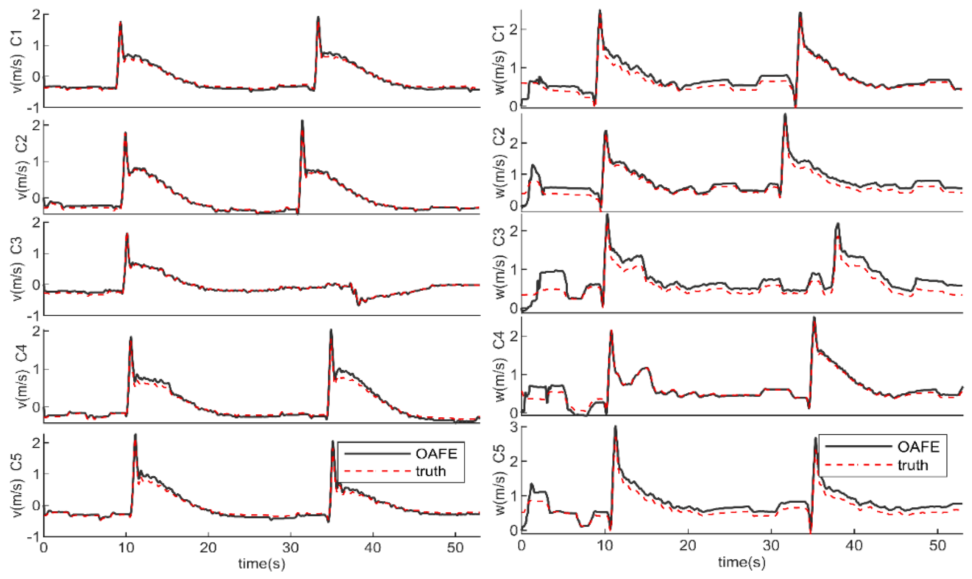
(3) To evaluate the OAFE, both 3D flight simulations and field tests were conducted. The simulation utilized an open-source flight dynamics model and a professional autopilot. The effectiveness of the estimation of relative velocity, flow angles, aerodynamic derivatives, and specific force is validated in this study.

The organization of this paper is as follows. Section 2 presents the mathematical models of flow angle estimation and introduces the theoretical frameworks employed in this paper. The proposed methods are discussed in detail in Section 3. In Section 4 and Section 5, the proposed method is evaluated through simulation and field tests conducted on a fixed-wing SUAV. Section 6 summarizes this study and indicates future work.

2. Problem Formulation

2.1. Kinematics Model

The definition of flow angles is illustrated in Figure 1, where $\alpha$ denotes the angle of attack and $\beta$ denotes the side slip angle. Generally, the relative velocity (also referred to as the velocity relative to air) of the aircraft to the surrounding airmass is labeled as ${\mathit{v}}_r$. The relative velocity is labeled as ${\mathit{v}}_r^b={\left[u,v,w\right]}^T$ in the body frame, as well as ${\mathit{v}}_r^n$ in the navigation frame. Below, the superscript $b$ denotes values in the body frame, $n$ denotes the navigation frame, and $a$ denotes the wind frame.

Once ${\mathit{v}}_r^b$ is known, the airspeed $V_a$, $\alpha$, $\beta$, and dynamic pressure $\overline{q}$ can be calculated by Equation (1) as follows:

$$\begin{array}{l}{V}_a=\parallel \left[u,v,w\right]\parallel \\ \alpha ={\tan }^{-1}\left(w/u\right)\\ \beta ={\sin }^{-1}\left(v/V_a\right)\\ \overline{q}=0.5\rho V_a^2\end{array}$$

(1)

where $\rho$ is the air density.

Wind significantly affects the air data of SUAVs flying at low speed. The ground velocity ${\mathit{v}}_g$ is not a good approximation of ${\mathit{v}}_r$ [24]. As shown in Equation (2), the so-called “wind triangle” denotes the relationship between ${\mathit{v}}_g$, wind velocity over ground ${\mathit{v}}_w$, and ${\mathit{v}}_r$ in the navigation frame [25]. To convert this to the body frame, the rotation matrix ${\mathit{C}}_n^b$ (refer to Appendix A.1) is introduced, as follows:

$$\begin{array}{l}{\mathit{v}}_r^n={\mathit{v}}_g^n-{\mathit{v}}_w^n\\ {\mathit{v}}_r^b=C_n^b\left({\mathit{v}}_g^n-{\mathit{v}}_w^n\right)\end{array}$$

(2)

Equation (2) provides a direct way to compute ${\mathit{v}}_r^b$. However, the standard sensor suite for SUAVs does not provide access to the real-time 3D wind field. Available engineering methods make zero-sideslip and horizontal wind field assumptions [26], which are practical approaches for macroscopic wind field estimation, but not beneficial for the precise estimation of ${\mathit{v}}_r^b$.

2.2. Dynamics Model

The SUAV’s aerodynamic force ${\mathit{F}}_a$ is given in [27], which, when decomposed in the wind frame, is denoted as follows:

$${\mathit{F}}_a={\left[-D,Y,-L\right]}^T=\overline{q}\overline{S}\left[\begin{array}{c}-\left(C_{D_0}+C_{D_{\alpha }}{\alpha }^2\right)\\ C_{Y_{\beta }}\beta +{C_Y}_{{\delta }_r}\\ -\left(C_{L_0}+C_{L_{\alpha }}\alpha +C_{L_q}q\overline{c}/2U_0+C_{L_{{\delta }_e}}{\delta }_e\right)\end{array}\right]$$

(3)

where $\overline{S}$ is the wing area, $C_{{\ast }_{\ast }}$ are aerodynamic derivatives, $\overline{c}$ is the mean aerodynamic chord, $U_0$ is the trim airspeed, $q$ is the pitch angular rate, and ${\delta }_e$ and ${\delta }_r$ are the elevator and rudder deflections.

For low-speed SUAVs, neglecting the effects of the Earth’s rotation and revolution, the dynamics are as follows:

$$m{\dot{\mathit{v}}}_g^b=m\left({\mathit{g}}^b+{\mathit{f}}^b\right)={\mathit{G}}^b+{\mathit{F}}_T^b+{\mathit{C}}_a^b{\mathit{F}}_a$$

(4)

where $m$ is the mass, ${\mathit{g}}^b$ is the gravitational acceleration, ${\mathit{f}}^b$ is the specific force, ${\mathit{G}}^b$ is gravity, ${\mathit{F}}_T^b$ is the thrust, and ${\mathit{C}}_a^b$ is the rotation matrix from the wind frame to the body frame given in Appendix A.1.

Considering SUAVs equipped with an IMU, ${\mathit{f}}^b$ can be measured directly. After cancelling out gravity, Equation (4) is represented as follows:

$$m{\mathit{f}}^{\mathrm{b}}={\mathit{F}}_T^b+{\mathit{C}}_a^b{\mathit{F}}_a$$

(5)

Equations (3) and (5) show the functional relation between aerodynamic derivatives and flow angles. Flow angles can be estimated on the premise that the exact aerodynamic derivatives of the SUAV are known [28].

2.3. Dynamics Simplification

SUAVs typically use non-vectorized propulsion. When decomposed in the body frame, ${\mathit{F}}_T^b$ has no component along the $y$ and $z$ axes. For small flow angle flights, Equations (3) and (5) yield the relationship among $\left[C_{Y_{\beta }}, {C_Y}_{{\delta }_r}, C_{L_0},C_{L_{\alpha }},C_{L_q},C_{L_{{\delta }_e}}\right]$, ${\mathit{v}}_r^b$, and ${\mathit{f}}^b$ as follows:

$$\begin{array}{l}{\mathit{f}}^{b,y}=\overline{q}\overline{S}(C_{Y_{\beta }}\beta +{C_Y}_{{\delta }_r})\cos \beta /m\\ {\mathit{f}}^{b,z}=-\overline{q}\overline{S}\left(C_{L_0}+C_{L_{\alpha }}\alpha +C_{L_q}{\displaystyle \frac{\overline{c}}{2U_0}}q+C_{L_{{\delta }_e}}{\delta }_e\right)\cos \alpha /m\end{array}$$

(6)

where ${\mathit{f}}^{b,y}$ and ${\mathit{f}}^{b,z}$ denote components of ${\mathit{f}}^b$ along the $y$ and $z$-axes.

2.4. Cubature Kalman Filter (CKF)

CKF is an accurate nonlinear filter that can be applied to solve high-dimensional nonlinear filtering problems with minimal computational efforts [29]. It uses a series of cubature points to propagate a priori and a posteriori statistical characteristic. As a result, the calculation of Jacobian matrix is avoided. In order to accommodate the fast maneuvers of aircraft, we used the square-root version of the CKF for its numerical stability. The square-root CKF algorithm is summarized as follows [30]:

(1) Time update

The predicted state ${\widehat{\mathbf{x}}}_{k\left|k-1\right.}$ and the square-root factor of the predicted error covariance $S_{k\left|k-1\right.}$, are computed using the estimated state ${\widehat{\mathbf{x}}}_{k-1\left|k-1\right.}$, the square root of state error covariance $S_{k-1\left|k-1\right.}$, and input ${\mathbf{u}}_{k-1}$, as follows:

$${\mathit{X}}_{i,k-1\left|k-1\right.}=S_{k-1\left|k-1\right.}{\lambda }_i+{\widehat{\mathbf{x}}}_{k-1\left|k-1\right.}$$

(7)

$${\mathit{X}}_{i,k\left|k-1\right.}^{\ast }=\mathbf{f}\left({\mathit{X}}_{i,k-1\left|k-1\right.},{\mathbf{u}}_{k-1}\right)$$

(8)

$${\widehat{\mathbf{x}}}_{k\left|k-1\right.}={\displaystyle \frac{1}{2n}}{\sum }_{i=1}^{2n}{\mathit{X}}_{i,k\left|k-1\right.}^{\ast }$$

(9)

$${\mathit{\chi }}_{k\left|k-1\right.}^{\ast }={\displaystyle \frac{1}{\sqrt{2n}}}\left[\begin{array}{ccc}{\mathit{X}}_{1,k\left|k-1\right.}^{\ast }-{\widehat{\mathbf{x}}}_{k\left|k-1\right.}& \dots & {\mathit{X}}_{2n,k\left|k-1\right.}^{\ast }-{\widehat{\mathbf{x}}}_{k\left|k-1\right.}\end{array}\right]$$

(10)

$$S_{k\left|k-1\right.}=\mathrm{Tria}\left(\left[\begin{array}{cc}{\chi }_{k\left|k-1\right.}^{\ast }& S_{Q,k-1}\end{array}\right]\right)$$

(11)

where $n$ is the dimension of the state $\mathbf{x}$, $i=\mathrm{1,2},\dots ,2n$, ${\lambda }_i=\sqrt{n}{\left[1\right]}_i$ and $\mathbf{f}\left(·\right)$ is the process equations. $\mathbf{T}\mathbf{r}\mathbf{i}\mathbf{a}\left(·\right)$ denotes a general triangularization algorithm, which returns a lower triangular matrix.

(2) Measurement update

The updated state ${\widehat{\mathbf{x}}}_{k\left|k\right.}$ and $S_{k|k}$ are estimated using ${\widehat{\mathbf{x}}}_{k\left|k-1\right.}$, $S_{k\left|k-1\right.}$, measurement ${\mathbf{z}}_k$, and the square root of the measurement error covariance $S_{R,k}$, as follows:

$${\mathit{X}}_{i,k\left|k-1\right.}=S_{k\left|k-1\right.}{\lambda }_i+{\widehat{\mathbf{x}}}_{k\left|k-1\right.}$$

(12)

$${\mathit{Z}}_{i,k\left|k-1\right.}=\mathbf{h}\left({\mathit{X}}_{i,k\left|k-1\right.},{\mathbf{u}}_k\right)$$

(13)

$${\widehat{\mathbf{z}}}_{k\left|k-1\right.}={\displaystyle \frac{1}{2n}}{\sum }_{i=1}^{2n}{\mathit{Z}}_{i,k\left|k-1\right.}$$

(14)

$${\mathcal{Z}}_{k|k-1}={\displaystyle \frac{1}{\sqrt{2n}}}\left[\begin{array}{ccc}{\mathit{Z}}_{1,k\left|k-1\right.}-{\widehat{\mathbf{z}}}_{k\left|k-1\right.}& \dots & {\mathit{Z}}_{2n,k\left|k-1\right.}-{\widehat{\mathbf{z}}}_{k\left|k-1\right.}\end{array}\right]$$

(15)

$$S_{zz,k\left|k-1\right.}=\mathrm{Tria}\left(\left[\begin{array}{cc}{\mathcal{Z}}_{k|k-1}& S_{R,k}\end{array}\right]\right)$$

(16)

$${\chi }_{k\left|k-1\right.}={\displaystyle \frac{1}{\sqrt{2n}}}\left[\begin{array}{ccc}{\mathit{X}}_{i,k\left|k-1\right.}-{\widehat{\mathbf{x}}}_{k\left|k-1\right.}& \dots & {\mathit{X}}_{2n,k\left|k-1\right.}-{\widehat{\mathbf{x}}}_{k\left|k-1\right.}\end{array}\right]$$

(17)

$$P_{xz,k\left|k-1\right.}={\chi }_{k\left|k-1\right.}{\mathcal{Z}}_{k\left|k-1\right.}^T$$

(18)

$$W_k=\left(P_{xz,k\left|k-1\right.}/S_{zz,k\left|k-1\right.}^T\right)/S_{zz,k\left|k-1\right.}$$

(19)

$${\widehat{\mathbf{x}}}_{k\left|k\right.}={\widehat{\mathbf{x}}}_{k\left|k-1\right.}+W_k\left({\mathbf{z}}_k-{\widehat{\mathbf{z}}}_{k\left|k-1\right.}\right)$$

(20)

$$S_{k\mid k}=\mathbf{Tria}\left(\left[\begin{array}{cc}{\chi }_{k\mid k-1}-W_k{\mathcal{Z}}_{k\mid k-1}& W_k{S}_{R,k}\end{array}\right]\right)$$

(21)

where $\mathbf{h}\left(·\right)$ is the measurement equation.

3. OAFE Method

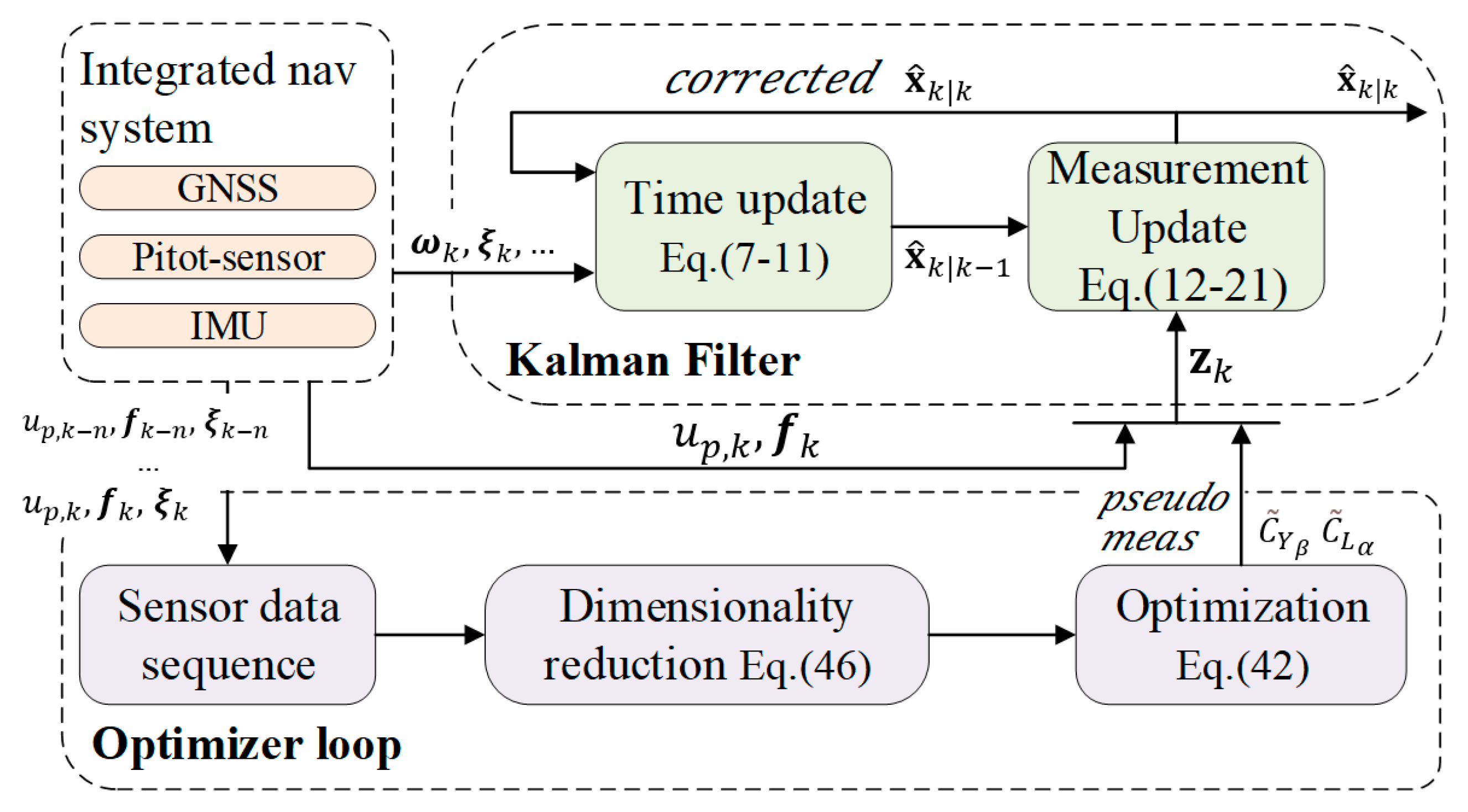
This study proposes an OAFE method for flow angle estimation comprising a filter loop and an optimizer loop (shown in Figure 2). The OAFE combines the benefits of both the filter and optimizer, with the filter serving as the main loop to generate flow angles.

A CKF filter was employed with low computational complexity and high frequency to capture states (${\mathbf{x}}_k$) changes caused by the SUAV maneuvering. The filter incorporates ${\tilde{\mathbf{z}}}_{p,k}$ from the optimizer loop as pseudo-measurements, thereby reducing cumulative errors and ensuring real-time outputs. The subscript $k$ in Figure 2 denotes values at time $t_k$.

Angular rates $\mathit{\omega }$, specific force $\mathit{f}$, pitot airspeed $u_p$, Euler angles $\mathit{\xi }$, and $\left[{\tilde{C}}_{Y_{\beta }}{{\tilde{C}}_L}_{\alpha }\right]$ are assumed to be available. Where $\mathit{\omega }$, $\mathit{f}$, $u_p$, $\mathit{\xi }$ are bias-corrected and provided by the integrated navigation system, $\left[{\tilde{C}}_{Y_{\beta }}{{\tilde{C}}_L}_{\alpha }\right]$ are real-time derivatives identified by the optimizer loop.

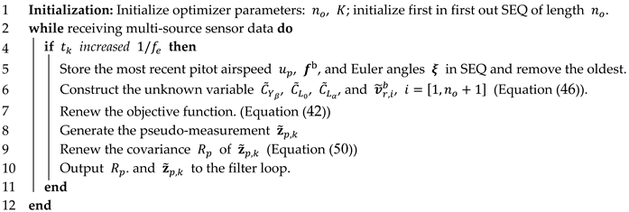
The optimizer loop generates aerodynamic derivatives at a frequency $f_e$, based on a sequence (SEQ) of past sensor data prior to the moment $t_k$ (as shown in Algorithm 1). The SEQ of the data is collected within a moving horizon, the length of which is $n_o+1$.

Algorithm 1 Optimizer for generating pseudo-measurement

3.1. Filter Loop

In this study, SUAVs are treated as nonlinear systems, as follows:

$$\begin{array}{c}\begin{array}{l}{\mathbf{x}}_{\mathrm{k}}=\mathbf{f}\left({\mathbf{x}}_{\mathrm{k}-1},{\mathbf{u}}_{\mathrm{k}-1}\right)+{\mathsf{\nu }}_{\mathrm{k}-1}\\ {\mathbf{z}}_{\mathrm{k}}=\mathbf{h}\left({\mathbf{x}}_{\mathrm{k}},{\mathbf{u}}_{\mathrm{k}},\right)+{\mathbf{w}}_{\mathrm{k}}\end{array}\end{array}$$

(22)

where $T$ is the sample time interval, ${\mathbf{v}}_{\mathrm{k}-1}$ and ${\mathbf{w}}_{\mathrm{k}}$ are the uncorrelated process and measurement Gaussian noise with zero means.

In this study, the filter loop is designed based on the dynamics and kinematics of the SUAV. Based on the CKF introduced in Section 2.4, the state (output) $\mathbf{x}$, input $\mathbf{u}$, and measurement $\mathbf{z}$ vectors are given as follows:

$$\mathbf{x}={\left[u,v,w,{C_L}_0,{C_L}_{\alpha },C_{L_q},C_{L_{{\delta }_e}},C_{Y_{\beta }}\right]}^T$$

(23)

$$\mathbf{u}={\left[p,q,r,\varphi ,\theta ,\psi ,{\mathit{f}}^{b,x},{\delta }_e,{\delta }_r\right]}^T$$

(24)

$$\begin{array}{c}\mathbf{z}={\left[u_p,{\mathit{f}}^{b,y},{\mathit{f}}^{b,z},{{\tilde{C}}_L}_{\alpha },{\tilde{C}}_{Y_{\beta }}\right]}^T\end{array}$$

(25)

Section 3.1.1 and Section 3.1.2 are explicit descriptions of the designed filter in the context of this study.

3.1.1. State Dynamic and Measurement

(1) State Dynamic Equations

The aerodynamic derivatives in state $\mathbf{x}$ use a static propagation model, as follows:

$$\left[\dot{{C_L}_0},\dot{{C_L}_{\alpha }},\dot{C_{L_q}},\dot{C_{L_{{\delta }_e}}},\dot{C_{Y_{\beta }}}\right]=0$$

(26)

The dynamic equation of the ${\mathit{v}}_r^b$ in state $\mathbf{x}$ can be obtained by differentiating Equation (2). Due to the high filter frequency, the wind field varies very little in a single period [31]; therefore, ${\dot{\mathit{v}}}_r^b$ can be represented as follows:

$$\begin{array}{l}\dot{{\mathit{v}}_r^b}=\dot{{\mathit{C}}_n^b}\left[{\mathit{v}}_g^n-{\mathit{v}}_w^n\right]+{\mathit{C}}_n^b\left[\dot{{\mathit{v}}_g^n}-{\dot{\mathit{v}}}_w^n\right]\\ \approx {\mathit{C}}_n^b\left({\mathit{\omega }}_{b\leftarrow n}^n\times \right){\mathit{v}}_r^n+{\mathit{C}}_n^b\dot{{\mathit{v}}_g^n}\\ =-{\mathit{C}}_n^b\left({\mathit{\omega }}_{n\leftarrow b}^n\times \right){\mathit{C}}_b^n{\mathit{C}}_n^b{\mathit{v}}_r^n+\dot{{\mathit{v}}_g^b}\\ =-\left({\mathit{\omega }}_{n\leftarrow b}^b\times \right){\mathit{v}}_r^b+\dot{{\mathit{v}}_g^b}\end{array}$$

(27)

where ${\mathit{\omega }}_{b\leftarrow n}$ represents the angular rate of the navigation frame relative to the body frame while ${\mathit{\omega }}_{n\leftarrow b}$ represents the opposite; ${\mathit{C}}_n^b$ is an orthogonal matrix, and the derivative of the rotation matrix ${\dot{\mathit{C}}}_n^b$ is given in [32].

Combining Equations (4) and (27), the UAV relative velocity is presented as follows:

$$\dot{{\mathit{v}}_r^b}=-\left({\mathit{\omega }}_{i\leftarrow b}^b\times \right){\mathit{v}}_r^b+\left({\mathit{G}}^b+{\mathit{F}}_T^b+{\mathit{C}}_a^b{\mathit{F}}_a\right)/m$$

(28)

where ${\mathit{\omega }}_{i\leftarrow b}^b\approx {\mathit{\omega }}_{n\leftarrow b}^b$ denotes the angular rates measured by IMU, the following expression is succinctly expressed as ${\mathit{\omega }}^b$. $\left({\mathit{\omega }}^b\times \right)$ is the antisymmetric matrix consisting of $\left[p,q,r\right]$ and is denoted by $\left({\mathit{\omega }}^b\times \right)=\left[\begin{array}{ccc}0& r& -q\\ -r& 0& p\\ q& -p& 0\end{array}\right]$.

Thus, the dynamic equations can be represented as follows:

$$\begin{array}{l}\dot{\mathbf{x}}={\left[\dot{u},\dot{v},\dot{w},\dot{{C_L}_0},\dot{{C_L}_{\alpha }},\dot{C_{L_q}},\dot{C_{L_{{\delta }_e}}},\dot{C_{Y_{\beta }}}\right]}^T\\ =-\left[\begin{array}{c}-\left({\mathit{\omega }}^b\times \right){\mathit{v}}_r^b\\ 0_{\left(5\times 1\right)}\end{array}\right]+\left[\begin{array}{c}{{\mathit{C}}_n^b{\mathit{g}}^n}_{\left(3\times 1\right)}\\ 0_{\left(5\times 1\right)}\end{array}\right]+\left[\begin{array}{c}\begin{array}{c}\begin{array}{c}\begin{array}{c}{\mathit{f}}^{b,x}\\ \overline{q}\overline{S}\left(C_{Y_{\beta }}\beta +{C_Y}_{{\delta }_r}{\delta }_r\right)\mathit{cos}\beta /m\\ -\overline{q}\overline{S}\left(C_{L_0}+C_{L_{\alpha }}\alpha +C_{L_q}{\displaystyle \frac{\overline{c}}{2V_a}}q+C_{L_{{\delta }_e}}{\delta }_e\right)\mathit{cos}\alpha /m\end{array}\end{array}\\ 0_{\left(5\times 1\right)}\end{array}\end{array}\right]\end{array}$$

(29)

where ${\mathit{f}}^{b,x}$ denotes the component of ${\mathit{f}}^b$ along the x-axes.

The cubature points propagate in Equation (8) according to the dynamic equations described in Equation (29).

(2) Measurement equations

The functional relation between $\left[u_p,{\tilde{C}}_{Y_{\beta }},{{\tilde{C}}_L}_{\alpha }\right]$ in corrector $\mathbf{z}$ and the state vector $\mathbf{x}$ is evident. Combined with Equation (6), the measurement equation $\mathbf{h}\left(·\right)$ in Equations (13) and (22) is precisely defined by Equation (30). where ${\delta }_r$, $q$, and ${\delta }_e$ are disregarded as they change at high frequency.

$$\mathbf{h}\left(\mathbf{x},\mathbf{u}\right)=\left[\begin{array}{c}\begin{array}{c}\begin{array}{c}u\\ \overline{q}\overline{S}{C}_{Y_{\beta }}\beta \cos \beta /m\\ -\overline{q}\overline{S}\left(C_{L_{\alpha }}\alpha +C_{L_0}\right)\cos \alpha /m\end{array}\\ C_{Y_{\beta }}\end{array}\\ C_{L_{\alpha }}\end{array}\right]$$

(30)

3.1.2. Filtering Noise

The IMU data used for the filters are bias-corrected. The estimation of these biases is conducted in the integrated navigation module, in which the bias of ${\mathit{\omega }}^b$ and ${\mathit{f}}^b$ are generally modeled as a first-order Markov process [15]. The main consideration in this study is the IMU noise, which affects both the state time update and the measurement update.

(1) Process error covariance

$S_{Q,k-1}$ in Equation (11) is a square-root factor of process error covariance $Q_{k-1}$, such that $Q_{k-1}=S_{Q,k-1}{S}_{Q,k-1}^T$. $Q_{k-1}$ is the covariance of process noise ${\mathsf{\nu }}_{\mathrm{k}-1}$ in Equation (22).

The process error covariance of ${\mathit{v}}_r^b$ is denoted as $Q_{v,k-1}$, and that of $\left[{C_L}_0,\cdots ,C_{Y_{\beta }}\right]$ is denoted as $Q_{C,k-1}$, such that $Q_{k-1}$ is expressed as follows:

$$Q_{k-1}=\left[\begin{array}{cc}{Q}_{v,k-1\left(3\times 3\right)}& 0_{\left(3\times 5\right)}\\ 0_{\left(5\times 3\right)}& Q_{C,k-1\left(5\times 5\right)}\end{array}\right]$$

(31)

Errors in the time update of ${\mathit{v}}_r^b$ are mainly due to input $\mathbf{u}$, arising from two terms ($A$) and ($B$), shown as follows:

$${\mathit{v}}_{r,k}^b={\mathit{v}}_{r,k-1}^b+{\int }_{t_{k-1}}^{t_k}\left[\begin{array}{c}\underset{\left(A\right)}{\underbrace{-\left({\mathit{\omega }}^b\times \right)\cdot {\mathit{v}}_r^b}}\\ +\underset{\left(B\right)}{\underbrace{{\mathit{C}}_n^b{\mathit{g}}^n}}+\left({\mathit{F}}_a^b+{\mathit{F}}_T^b\right)/m\end{array}\right]dt$$

(32)

In this study, the noises associated with ($A$) and ($B$) are considered to be independent of each other within a filter period and can be evaluated separately. Then, the process error covariance of ${\mathit{v}}_r^b$ can be expressed as follows:

$$Q_{v,k-1}=Q_{v,k-1}^A+Q_{v,k-1}^B$$

(33)

The propagation residual ${\mathit{e}}_A$ of ${\mathit{v}}_r^b$ caused by the term ($A$) can be expressed as follows:

$${\mathit{e}}_A={\int }_{t_{k-1}}^{t_k}-\left({\mathit{\delta }}_{{\mathit{\omega }}^b}\times \right)\cdot {\mathit{v}}_{r,k-1}^{b}dt$$

(34)

where ${\mathit{\delta }}_{{\mathit{\omega }}^b}$ denotes the noise vector of the gyroscope.

According to the derivation in Appendix A.2, $Q_{v,k-1}^A$ can be expressed as follows:

$$Q_{\mathit{v},k-1}^A=\left({\mathit{v}}_{r,k-1}^b\times \right){\mathit{\sigma }}_{{\mathit{\omega }}^b}^2{\left({\mathit{v}}_{r,k-1}^b\times \right)}^T\cdot T$$

(35)

where ${\mathit{\sigma }}_{{\mathit{\omega }}^b}^2$ represents the angular rate variance, which is detailed in Section 4.

For small and low-speed SUAVs, the variation of ${\mathit{g}}^n$ can be ignored and $Q_{v,k-1}^B$ mainly results from attitude errors as Equation (36). The derivation is detailed in Appendix A.2, as follows:

$$Q_{\mathit{v},k-1}^B={\mathit{C}}_n^b\left({\mathit{g}}^n\times \right){\mathit{\sigma }}_{\mathit{\xi }}^2\left({\mathit{g}}^n\times \right){\mathit{C}}_b^n·T$$

(36)

where ${\mathit{\sigma }}_{\mathit{\xi }}^2$ represents the Euler angles variance, which is detailed in Section 4.

(2) Measurement noise

$S_{R,k}$ in Equation (16) is a square-root factor of the measurement error covariance $R_k$, such that $R_k=S_{R,k}{S}_{R,k}^T$. $R_k$ is the covariance of measurement noise ${\mathbf{r}}_{\mathrm{k}}$, and is expressed as follows:

$$R_k=\left[\begin{array}{cc}{R_s}_{\left(3\times 3\right)}& 0_{\left(3\times 2\right)}\\ 0_{\left(2\times 3\right)}& {R_p}_{\left(2\times 2\right)}\end{array}\right]$$

(37)

where $R_s$ is constructed from the sensor noise and $R_p$ denotes the error covariance of real-time derivatives from the optimizer loop at the time $t_k$.

$R_s$ is represented as follows:

$$R_s=\mathbf{d}\mathbf{i}\mathbf{a}\mathbf{g}\left(\left[{\sigma }_{u_p}^2,{\sigma }_{{\mathit{f}}^{b,y}}^2,{\sigma }_{{\mathit{f}}^{b,z}}^2\right]\right)$$

(38)

where the symbol “$\mathbf{d}\mathbf{i}\mathbf{a}\mathbf{g}\left(a\right)$” stands for a diagonal matrix with $a$ on the main diagonal; $\left[{\sigma }_{u_p}^2,{\sigma }_{{\mathit{f}}^{b,y}}^2,{\sigma }_{{\mathit{f}}^{b,z}}^2\right]$ denote the variance of $\left[u_p,{\mathit{f}}^{b,y},{\mathit{f}}^{b,z}\right]$, and the associated sensor noise is detailed in Section 4.

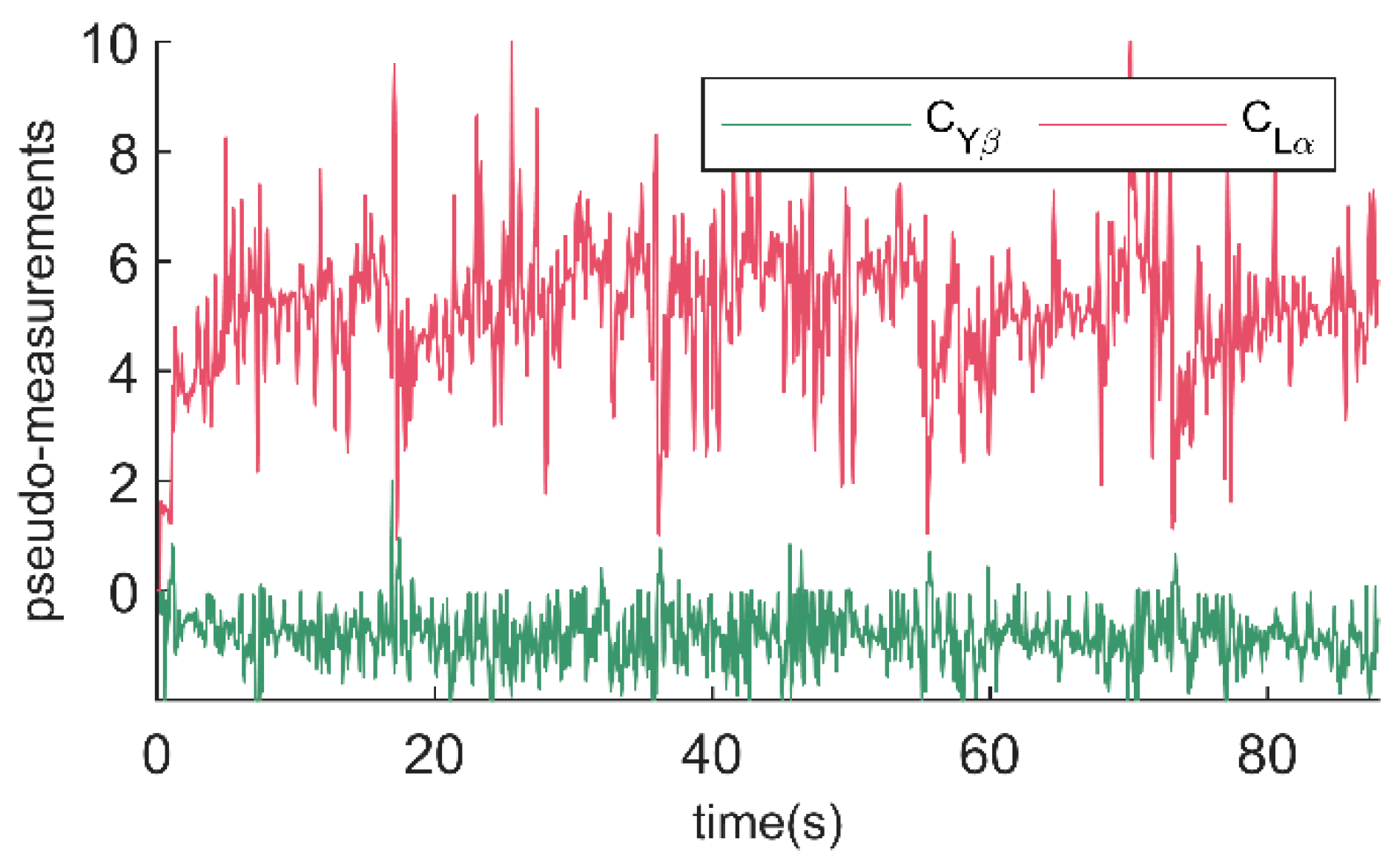
As mentioned earlier, derivatives exhibit a high level of noise. Real-time [${\tilde{C}}_{Y_{\beta }} {{\tilde{C}}_L}_{\alpha }$] generated from the optimizer loop in flight tests are shown in Figure 3. To use them as pseudo-measurements, their noise level $R_p$ is detailed in the design of the optimizer loop (shown in Section 3.2.3).

3.2. Optimizer Loop

The main difficulty faced by the optimizer loop is that the flow angles are unknown since they are exactly the states to be estimated by the OAFE.

Based on an SEQ of past sensor data collected over multiple periods, the optimizer loop determines a set of aerodynamic derivatives that satisfy the following two conditions:

(1) The SUAV flight states satisfy the motion-continuity rule (Equation (28)) [33];

(2) The air data parameters (including ${\mathit{v}}_r^b$) and aerodynamic parameters determine the SUAV’s forces (Equation (6)) [34].

3.2.1. Objective Function

Assuming there is a functional relation between the input and output data, this optimization aims to determine the functional relation that minimizes the error, as follows:

$$\mathit{Y}=\mathit{W}\left(\mathsf{\Theta }\right)+\mathbf{w}$$

(39)

where $\mathit{Y}$ represents the output and $\mathit{W}\left(·\right)$ represents the input. $\mathsf{\Theta }$ is the unknown variable to be determined.

More precisely, $\mathit{Y}$ and $\mathsf{\Theta }$ are defined as follows:

$$\left\{\begin{array}{l}\mathit{Y}={\left[u_p,{\mathit{f}}^{b,y},{\mathit{f}}^{b,z}\right]}^T\\ \mathit{\Theta }={\left[\tilde{u},\tilde{v},\tilde{w},{\tilde{C}}_{Y_{\beta }},{\tilde{C}}_{L_0},{\tilde{C}}_{L_{\alpha }}\right]}^T\end{array}\right.$$

(40)

where $\left[\tilde{u},\tilde{v},\tilde{w}\right]$ denote the components of ${\tilde{\mathit{v}}}_r^b$ to be determined and $\left[{\tilde{C}}_{Y_{\beta }},{\tilde{C}}_{L_0},{\tilde{C}}_{L_{\alpha }}\right]$ denote the derivatives to be determined.

$\mathit{W}\left(·\right),$ in Equation (39), can be represented as Equation (41). The aerodynamic forces due to $\left[{\delta }_r,q,{\delta }_e\right]$ are also ignored, as follows:

$$\underset{\mathit{Y}}{\underbrace{\left[\begin{array}{c}{u}_p\\ {\mathit{f}}^{b,y}\\ {\mathit{f}}^{b,z}\end{array}\right]}}=\underset{\mathit{W}\left(\mathit{\Theta }\right)}{\underbrace{\left[\begin{array}{c}\left[\begin{array}{c}\mathrm{1,0},0\end{array}\right]{\left[\tilde{u},\tilde{v},\tilde{w},\right]}^T\\ \mathcal{F}\left(\tilde{u},\tilde{v},\tilde{w},{\tilde{C}}_{Y_{\beta }},{\tilde{C}}_{L_0},{\tilde{C}}_{L_{\alpha }}\right)\\ \mathcal{G}\left(\tilde{u},\tilde{v},\tilde{w},{\tilde{C}}_{Y_{\beta }},{\tilde{C}}_{L_0},{\tilde{C}}_{L_{\alpha }}\right)\end{array}\right]}}+\mathbf{w}$$

(41)

where $\mathcal{F}\left(·\right)$ and $\mathcal{G}\left(·\right)$ denote the functional relation among $\tilde{u}$, $\tilde{v}$, $\tilde{w}$, ${\tilde{C}}_{Y_{\beta }}$, ${\tilde{C}}_{L_0}$, ${\tilde{C}}_{L_{\alpha }}$, and $\left[{\mathit{f}}^{b,y},{\mathit{f}}^{b,z}\right]$ in Equation (6); $\mathbf{w}$ denotes the associated measurement noise.

At time $t_k$, when extending Equation (41) to $n_o+1$ periods, there are historical measurement sequences, as follows:

$$\left\{\begin{array}{l}{u}_{p,k-n_o},u_{p,k-n_o+1},\dots ,u_{p,k}\\ {\mathit{f}}_{k-n_o}^{b,y},{\mathit{f}}_{k-n_o+1}^{b,y},\dots ,{\mathit{f}}_k^{b,y}\\ {\mathit{f}}_{k-n_o}^{b,z},{\mathit{f}}_{k-n_o+1}^{b,z},\dots ,{\mathit{f}}_k^{b,z}\end{array}\right.,$$

and the variable sequences are ${\mathit{\Theta }}_{k-n_o}, {\mathit{\Theta }}_{k-n_o+1}, \dots {\mathit{\Theta }}_k$.

At time $t_k$, subscript $\left[k-n_o, k-n_o+1, \dots , k\right]$ is marked as $\left[1, 2, \dots , n_o+1\right]$ for easy expression. Finally, the optimizer loop finds the unknown ${\mathit{\Theta }}_1, {\mathit{\Theta }}_2, \dots {\mathit{\Theta }}_{n_o+1}$, by minimizing the objective function at time $t_k$, as follows:

$$J\left(\mathit{\Theta }\right)=\underset{{\mathit{\Theta }}_i}{\min }{\sum }_{i=1}^{n_o+1}K·{\left[\begin{array}{c}{\mathit{Y}}_i-\mathit{W}\left({\mathit{\Theta }}_i\right)\\ {\mathit{\Theta }}_1-{\widehat{\mathit{\Theta }}}_{pre}\end{array}\right]}^T\left[\begin{array}{c}{\mathit{Y}}_i-\mathit{W}\left({\mathit{\Theta }}_i\right)\\ {\mathit{\Theta }}_1-{\widehat{\mathit{\Theta }}}_{pre}\end{array}\right]$$

(42)

where $K$ denotes the weight vector; one available $K$ for testing in this study is $K=\left[1, 4, 1, 0, 0, 0, 1.5, 1, 1\right]$; ${\widehat{\mathit{\Theta }}}_{pre}$ denotes the previous estimates at time $t_{k-n_o}$ from the filter loop.

Based on our tests using the selected sensors with a data acquisition frequency of 10 Hz, it was considered that a time window width of $n_o=5$ in Equation (42) was appropriate. As the acquisition frequency increases, it is advisable to correspondingly increase the value of $n_o$. Similarly, if the sensor accuracy improves,$n_o$ can be also increased.

In this study, the Levenberg–Marquardt algorithm was employed to conduct the optimization task. To ensure prompt optimization outcomes, a maximum of 30 iterations was set for each optimization period.

3.2.2. Improving Optimization Efficiency

(1) Variable dimensionality reduction

At time $t_k$, $[{\tilde{C}}_{Y_{\beta }}$, ${\tilde{C}}_{L_0}$, ${\tilde{C}}_{L_{\alpha }}]$ in ${\mathit{\Theta }}_i$ across the time window are treated as constants. In contrast, ${\tilde{\mathit{v}}}_{r,i}^b$ is rapidly changing. In order to reduce the dimensionality, the unknown variables ${\tilde{\mathit{v}}}_{r,i}^b$ in ${\mathit{\Theta }}_i$ are treated as functions of ${\tilde{\mathit{v}}}_{r,1}^b$.

In addition, since the online resolution of Equation (42) uses an optimization algorithm, the optimization process computes ${\tilde{\mathit{v}}}_{r,i}^b$ multiple times, utilizing distinct $\left[{\widehat{u}}_1,{\tilde{v}}_1,{\tilde{w}}_1\right]$. In order to avoid a high number of repetitive recursive operations, the increment of ${\tilde{\mathit{v}}}_r^b$ is used to construct the unknown ${\tilde{\mathit{v}}}_{r,i}^b$ (shown in Figure 4).

Neglecting the variation of the wind field during the time window, the equation is first established in the navigation frame as follows:

$${\tilde{\mathit{v}}}_{r,i}^n={\tilde{\mathit{v}}}_{r,1}^n+∆{\mathit{v}}_i^n, i=1, 2, \dots , n_o+1$$

(43)

where $∆{\mathit{v}}_i^n$ denotes the increment of ${\mathit{v}}^n$ within the time window $\left[t_1,t_i\right]$.

The discrete form of pre-integration [35] is utilized to approximate $∆{\displaystyle {\mathit{v}}_i^n}$ as follows:

$$∆{\mathit{v}}_i^n={\sum }_{j=1}^{i-1}\left[{\mathit{C}}_b^n\left(j\right){\mathit{f}}_j^b+{\mathit{g}}^n\right]·T, i=1, 2, \dots , n_o+1$$

(44)

where the script $j$ denotes the values at time $t_j$ and ${\mathit{C}}_b^n\left(j\right)$ represents the rotation matrix at time $t_j$.

As a result, the constructed sequence ${\tilde{\mathit{v}}}_{r,i}^n$ naturally satisfies the continuity rule expressed in Equation (28). When decomposed in the body frame, Equation (43) is expressed as follows:

$${\tilde{\mathit{v}}}_{r,i}^b={\mathit{C}}_n^b\left(i\right)\left[{\mathit{C}}_b^n\left(1\right){\tilde{\mathit{v}}}_{r,1}^b+∆{\mathit{v}}_i^n\right], i=1, 2, \dots , n_o+1$$

(45)

(2) Minimize redundant operations

Combining Equations (44) and (45) yields Equation (46). Based on Equation (46), it is possible to directly construct the unknown variables of sequence ${\tilde{\mathit{v}}}_{r,i}^b$ instead of the repetitive recursive operations. At time $t_k$, only ${\tilde{v}}_1$ and ${\tilde{w}}_1$ are unknown variables in sequence ${\tilde{\mathit{v}}}_{r,i}^b$, as follows:

$$\begin{array}{l}{\tilde{\mathit{v}}}_{r,i}^b={\mathit{C}}_n^b\left(i\right){\mathit{C}}_b^n\left(1\right){\tilde{\mathit{v}}}_{r,1}^b+∆{\mathit{v}}_{r,i}^b, i=1, 2, \dots , n_o+1\\ ∆{\mathit{v}}_{r,i}^b={\mathit{C}}_n^b\left(i\right)\sum _{j=1}^{i-1}\left[{\mathit{C}}_b^n\left(j\right){\mathit{f}}_j^b+{\mathit{g}}^n\right]·T\end{array}$$

(46)

According to Equation (46), the sequence ${\tilde{\mathit{v}}}_{r,i}^b$ are computed using ${\mathit{C}}_n^b\left(i\right)$ and $∆{\mathit{v}}_{r,i}^b$. Once ${\mathit{C}}_n^b\left(i\right)$ and $∆{\mathit{v}}_{r,i}^b$ are obtained, they remain constant throughout the optimization process at time $t_k$.

Moreover, Equation (47) is derived from Equation (46). With Equation (47), the sequence ${∆{\mathit{v}}_{r,i}^b|}_{k+1}$ at time $t_{k+1}$ can be quickly obtained based on the sequence ${∆{\mathit{v}}_{r,i}^b|}_k$ at time $t_k$. Thus, the optimization task at time $t_{k+1}$ can start quickly, avoiding the repetitive computation of $∆{\mathit{v}}_{r,i}^b$, as follows:

$$\begin{array}{c}{∆{\mathit{v}}_{r,i}^b|}_{k+1}={{\mathit{C}}_n^b\left(i\right)|}_{k+1}\left\{{\mathit{C}}_b^n{\left(i\right)|}_k·{∆{\mathit{v}}_{r,i+1}^b|}_k+\left[{{\mathit{C}}_b^n\left(i-1\right)|}_{k+1}·{{\mathit{f}}_{i-1}^b|}_{k+1}-{\mathit{C}}_b^n{\left(1\right)|}_k·{{\mathit{f}}_1^b|}_k\right]·T\right\}, \hfill \\ i=\mathrm{1,2},\dots ,n_o+1\hfill \end{array}$$

(47)

when $i=n_o+1$, ${∆{\mathit{v}}_{r,i+1}^b|}_k=0.$

3.2.3. Noises of Selected Derivatives

The sequence ${\tilde{\mathit{v}}}_{r,i}^b$ can be calculated through Equation (46) at time $t_k$, once $\left[\tilde{v},\tilde{w}\right]$ are determined. It is easy to calculate sequences $\left[Q_1, \dots , Q_{n_o+1}\right]$, $\left[{\mathrm{\alpha }}_1, \dots , {\mathrm{\alpha }}_{n_o+1}\right]$, and $\left[{\beta }_1, \dots , {\beta }_{n_o+1}\right]$ from time $t_{k-n}$ to $t_k$ according to Equation (1).

The error variance is thus expressed as follows:

$${\sigma }^2\left({{\tilde{C}}_L}_{\alpha }\right)={\displaystyle \frac{1}{n_o+1}}{\sum }_{i=1}^{n_o+1}{\left(\left({\displaystyle \frac{m{\mathit{f}}_i^{b,z}}{Q_{i}S}}-{{\tilde{C}}_L}_0\right)/{\alpha }_i-{{\tilde{C}}_L}_{\alpha }\right)}^2$$

(48)

$${\sigma }^2\left({\tilde{C}}_{Y_{\beta }}\right)={\displaystyle \frac{1}{n_o+1}}{\sum }_{i=1}^{n_o+1}{\left({\displaystyle \frac{m{\mathit{f}}_i^{b,y}}{Q_{i}S{\beta }_i}}-{{\tilde{C}}_L}_{\beta }\right)}^2$$

(49)

On the other hand, considering that the flight control system counteracts the perturbations required to excite the SUAV dynamics [36], the error covariance of the estimated derivatives is weighted by normalized flow angle variations within the time window. Therefore, $R_p$ in Equation (37) is set as follows:

$$R_p=\left[\begin{array}{cc}{\sigma }^2\left({{\tilde{C}}_L}_{\alpha }\right)/{\mathrm{e}}^{∆\mathrm{\alpha }}& 0\\ 0& {\sigma }^2\left({{\tilde{C}}_L}_{\beta }\right)/{\mathrm{e}}^{∆\mathrm{\beta }}\end{array}\right]$$

(50)

where $∆\mathrm{\alpha }=\max \left({\mathrm{\alpha }}_{k-n},\dots ,{\mathrm{\alpha }}_k\right)-\min \left({\mathrm{\alpha }}_{k-n},\dots ,{\mathrm{\alpha }}_k\right)$, $∆\beta =\max \left({\beta }_{k-n},\dots ,{\beta }_k\right)-\min \left({\beta }_{k-n},\dots ,{\beta }_k\right)$, and $\mathrm{e}$ is a natural constant.

4. Simulation

In this study, the OAFE method was first tested using a flight simulation. The flight simulation provides a fundamental guarantee for field trials, allows for more scenarios to be simulated, and facilitates more detailed and refined testing of the method in the future. The ideas for evaluations in the simulation are shown in

Table 1. Validation methods.

OAFE Estimates	Reference for Simulation
$u, v, w, \alpha , \beta , {\mathit{f}}^b$	Truth values from the HIL Syst
$C_L, C_{\beta }, {C_L}_{\alpha }, C_{Y_{\beta }}$	Derivatives of SUAV in the HIL Syst

. Both the flow angles and aerodynamic parameters estimated by the OAFE were evaluated. To enhance readability, the aerodynamic derivatives were synthesized into aerodynamic coefficients for presentation.

4.1. Initialization of OAFE

To start the OAFE, the initial states ${\mathbf{x}}_0$, and the initial error covariance $P_0$ of ${\mathbf{x}}_0$ were set as follows:

$${\mathbf{x}}_0={\left[u_{p,0}, 0, 0, -2, -10, 0, 0\right]}^T$$

(51)

$$P_0=diag\left(\left[5^2, 3^2, 3^2, 0.01, 0.01, 0.01, 0.01\right]\right)$$

(52)

where the $u_{p,0}$ is the pitot airspeed when the filter starts, and $S_{0,0}$ in Section 2.4 is the square root of $P_0$.

Referring to the parameters of onboard sensors, the noise characteristics of the inputs and measurements are shown in

Table 2. Noise characteristics of the OAFE.

Input Noise ${\mathit{\sigma }}^2$		$\mathbf{Measurement} \mathbf{Noise} {\mathit{\sigma }}^2$
$p$	${0.00109}^2 {\left(\mathrm{r}\mathrm{a}\mathrm{d}/\mathrm{s}\right)}^2$	$u_p$	${0.2}^2 {\left(\mathrm{m}/\mathrm{s}\right)}^2$
$q$	${0.00109}^2 {\left(\mathrm{r}\mathrm{a}\mathrm{d}/\mathrm{s}\right)}^2$	${\mathit{f}}^{b,y}$	$4\times {10}^{-5} {\left(\mathrm{m}/{\mathrm{s}}^2\right)}^2$
$r$	${0.00109}^2 {\left(\mathrm{r}\mathrm{a}\mathrm{d}/\mathrm{s}\right)}^2$	${\mathit{f}}^{b,z}$	$4\times {10}^{-5} {\left(\mathrm{m}/{\mathrm{s}}^2\right)}^2$
$\varphi$	${0.014}^2 {\mathrm{r}\mathrm{a}\mathrm{d}}^2$	${{\tilde{C}}_L}_{\alpha }$	$R_{p,11}$ (Equation (50))
$\theta$	${0.014}^2 {\mathrm{r}\mathrm{a}\mathrm{d}}^2$	${\tilde{C}}_{Y_{\beta }}$	$R_{p,22}$ (Equation (50))
$\psi$	${0.009}^2 {\mathrm{r}\mathrm{a}\mathrm{d}}^2$
${\delta }_e$	$8\times {10}^{-5} \mathrm{r}\mathrm{a}{\mathrm{d}}^2$
${\delta }_r$	$8\times {10}^{-5} \mathrm{r}\mathrm{a}{\mathrm{d}}^2$

. The values of $\varphi$, $\theta$, and $\psi$ provided are reference values; in practice, they are determined by the integrated navigation system and are updated in real time.

The process error covariance of aerodynamic parameters $Q_C$ in Equation (31) was set as follows:

$$Q_{C,k-1}={0.01}^{2}diag\left(\left[{0.1}^2,1^2,1^2,1^2,1^2\right]\right)$$

(53)

4.2. HIL Simulation System

To accurately replicate real-world conditions, a hardware-in-loop (HIL) simulation was implemented. The simulation employed an onboard autopilot (comprising both the hardware Pixhawk and software px4) and an onboard computer system NX3 (running the OAFE) identical to those used in an actual SUAV. A workstation was used for the flight simulation and a control station was used for the mission setup. The hardware configuration is depicted in Figure 5.

We modeled the sensors of the test SUAV in HIL based on the noise characteristics from the real onboard sensors shown in

Table 3. Sensor’s performance parameters.

Sensors	Type	Noise/Error
BMI160	IMU	$0.014°/\mathrm{S}/\sqrt{\mathrm{H}\mathrm{z}}$
		$150 \mathrm{\mu }\mathrm{g}/\sqrt{\mathrm{H}\mathrm{z}}$
MS5525	pressure sensor and pitot tube	$\pm 0.84 \mathrm{P}\mathrm{a}$
HEX Here3	GPS Module	$\mathrm{pos}: 2.5 \mathrm{m}$ $\mathrm{vel}: 0.1 \mathrm{m}/\mathrm{s}$

.

The simulation framework is illustrated in Figure 6. To start the flight simulation, JSBSim first instantiates the SUAV system model and configures the associated parameters. Subsequently, it sets the initial position, attitude, and velocity of the SUAV.

The following processes occurred during each simulation period: ① the JSBSim received commands from the px4 autopilot to control the SUAV’s actuators. Subsequently, it then updated the aerodynamic forces and moments of the model and proceeded with the kinematic solution; ② The px4 autopilot operated on the Pixhawk hardware platform. It acquired sensor data from JSBSim, fused the data for navigation, and generated control commands according to the preset mission; and ③ the OAFE accepted ${\mathit{f}}^b$, $\mathit{\xi }$, ${\mathit{\omega }}^b$, and $u_P$ from the px4 and estimated $\left[u, v, w\right]$, $\left[\alpha ,\beta \right]$ and $\left[{C_L}_0,{C_L}_{\alpha },C_{L_q},C_{L_{{\delta }_e}},C_{Y_{\beta }}\right]$.

4.3. Simulation Setup

4.3.1. Simulation Scenes

Wind is an important topic in flight mechanics and the aerodynamic forces of SUAVs are highly sensitive to the wind field. In this study, five different 3D wind fields were set up in the flight simulation. These five wind fields were defined in the navigation frame, including the crosswind, headwind, tailwind, and updraft, as shown in

Table 4. Wind fields set-up in flight simulation.

Wind Field Conditions	Wind Fields (m/s)
Case 1	$\left[0, 0, 0\right]$
Case 2	$\left[0, 3, 0\right]$
Case 3	$\left[0, 0,-3\right]$
Case 4	$\left[0, 2.2,-2.2\right]$
Case 5	$\left[-6, 0, 0\right]$

.

The wind velocity ${\mathit{v}}_w^n$ was assumed to be the sum of a low-frequency part ${\mathit{v}}_s^n$ and a high-frequency turbulent part ${\mathit{v}}_t^n$. The ${\mathit{v}}_s^n$ was assumed to be slowly time-varying as ${\dot{\mathit{v}}}_s^n\approx 0$. The ${\mathit{v}}_t^n$ is modeled by the Dryden wind model¹⁴ as follows:

$${\mathit{v}}_{t,k+1}^n={\mathit{v}}_{t,k}^n-T{V}_a\left({\mathit{v}}_t^n\circ {\displaystyle \frac{1}{{\mathit{L}}_k}}\right)+{\mathit{\sigma }}_{{\mathit{v}}_t}\circ \sqrt{2T{V}_a/{\mathit{L}}_k}\circ {\mathbf{v}}_{{\mathit{v}}_t}$$

(54)

where ${\mathit{L}}_k$ is the spatial wavelength, ${\mathit{\sigma }}_{{\mathit{v}}_t}$ is the noise amplitude, ${\mathbf{v}}_{{\mathit{v}}_t}$ is the Gaussian white noise, and “$\circ$” denotes the Hadamard product.

As depicted in Figure 7, the simulation flight path primarily consisted of a straight flight and turns; the px4 autopilot controlled the SUAV to fly along the path at a cruise speed of 30 m/s under different wind field conditions. Data from the red route segments were intercepted for analysis.

4.3.2. Simulation Process

In real-world scenarios, SUAVs commonly employ autopilots to ensure safety and efficient flight operations in line with the mission. Consequently, the flow angles are often constrained within a narrow range, making it challenging to excite the dynamics of the SUAV. To replicate realistic conditions in this study, the “Mission” mode of the px4 autopilot was utilized for verification purposes. The attitude variations of the SUAV in the five scenarios are depicted in Figure 8.

During the simulation implementation, we also collected $\left[u,v,w\right]$ and $\left[\alpha ,\beta \right]$ from JSBSim, which jointly, with the preset aerodynamic derivatives, served as the reference for validating the OAFE method.

4.4. Simulation Results and Analysis

The OAFE method was evaluated by comparing the estimated values of ${\mathit{v}}_r^b$, the coefficient of side force $C_Y$, the coefficient of lift $C_L$, ${C_L}_{\alpha },C_{Y_{\beta }}$, and ${\mathit{f}}^{b,y},{\mathit{f}}^{b,z}$ (labeled as “OAFE”) with the reference values provided by the HIL system (labeled as “truth”). In the simulations, the OAFE output frequency was set to 20 Hz. Data from two complete turns along the above flight path were collected to assess the performance of the OAFE method. All the estimated values were highly accurate (Figure 9, Figure 10 and Figure 11).

As mentioned in Section 3.2, the air data parameters (including ${\mathit{v}}_r^b$) and aerodynamic parameters determine its aerodynamic force. A comparison was made between the calculated values of ${\mathit{f}}^{b,y}$ and ${\mathit{f}}^{b,z}$(obtained from the estimated $\left[u,v,w\right]$ and aerodynamic parameters) with the truth values. This comparison is illustrated in Figure 12.

As shown in

Table 5. Root mean square errors of estimates.

Case	$\mathit{v}$ (m/s)	$\mathit{w}$ (m/s)	$\mathit{\beta }$ (°)	$\mathit{\alpha }$ (°)
C1	0.038	0.127	0.072	0.239
C2	0.041	0.151	0.076	0.234
C3	0.028	0.137	0.051	0.257
C4	0.076	0.091	0.141	0.170
C5	0.069	0.155	0.129	0.293

, the OAFE method demonstrates a strong efficacy in estimating $v$, $w$, $\beta$, and $\alpha$, across five distinct wind field conditions. The root mean square error (RMSE) of $\alpha$ varies less under different wind field conditions, whereas the accuracy of $\beta$ is higher during flights without crosswinds.

$C_{L_{\alpha }}$ and $C_{Y_{\beta }}$ are theoretically constant values when $\alpha$ and $\beta$ are small. Thus, the real-time estimates of $C_{L_{\alpha }}$ and $C_{Y_{\beta }}$ obtained from the OAFE should converge to their true values, respectively. More importantly, in this study, the convergence of $C_{L_{\alpha }}$ and $C_{Y_{\beta }}$ with different initial values can be a factor in demonstrating the feasibility of the OAFE. The simulation results (shown in Figure 13) demonstrate that $C_{L_{\alpha }}$ shows good convergence with different initial values in C5.

5. Field Tests

The ideas for evaluation in the flight tests are shown in

Table 6. Validation methods for flight tests.

OAFE Estimates	Reference for Field Test
$u, v, w$ $\alpha , \beta$	Model-aided method
$C_L, C_{\beta }, {C_L}_{\alpha }, C_{Y_{\beta }}$	Parameters from a CFD work; Derivatives convergence
$f^{b,y}, f^{b,z}$	$f^{b,y}, f^{b,z}$ measured by IMU

. In the flight tests, the model-aided method provides reference values for $\alpha$ and $\beta$, as it is an extensively researched method with an accuracy within 0.5° and 1° [5,20,23]. What we aim to demonstrate in the field tests is that the proposed method achieves the estimation of flow angles without the prior acquisition of aerodynamic parameters, rather than achieving superior estimation accuracy.

Before conducting the field test, an aerodynamic derivatives model was developed for the test SUAV [37]. This model serves two purposes in the field tests, as follows: to provide reference aerodynamic parameters; and to complete a model-aided estimation. Appendix A.3 provides detailed aerodynamic parameters.

5.1. SUAV for Flight Tests

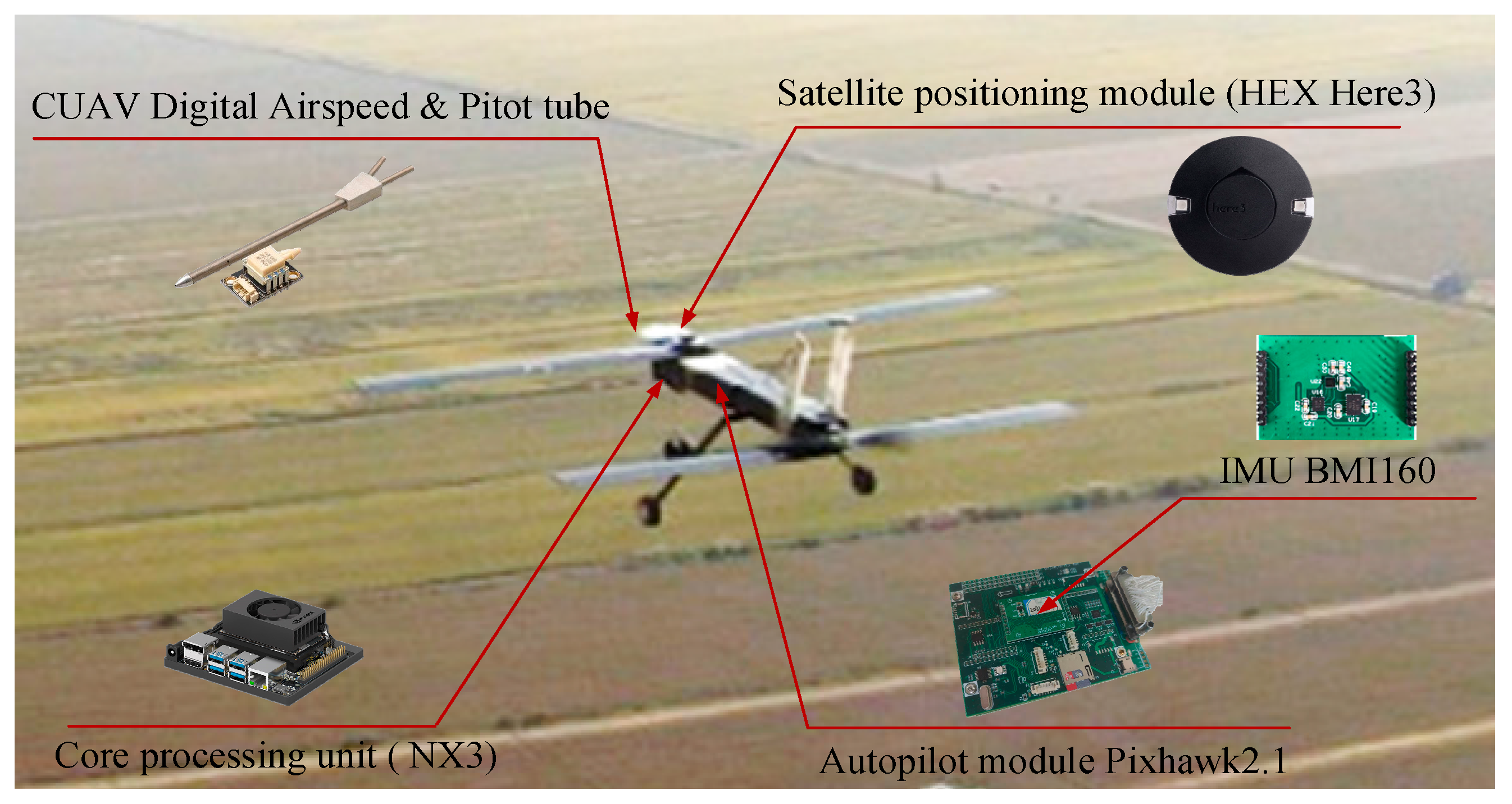
The Sula89 SUAV, employed for conducting the field tests, is presented in Figure 14. The Sula89 adopts a tandem layout with a high aspect ratio and equal-chord straight wings. The vertical tails act as a lateral stabilizer. Detailed geometric characteristics of the Sula89 are shown in

Table 7. Geometric characteristics of the Sula89.

Parameters	Values
Aerodynamic configuration	Tandem wing
Fuselage length	0.92 m
Wingspan	1.56 m
Reference area	$0.26 {\mathrm{m}}^2$
Aspect ratio	11
Mean aerodynamic chord	0.19 m
Mass	8.9 kg
Cruise speed	30 m/s

.

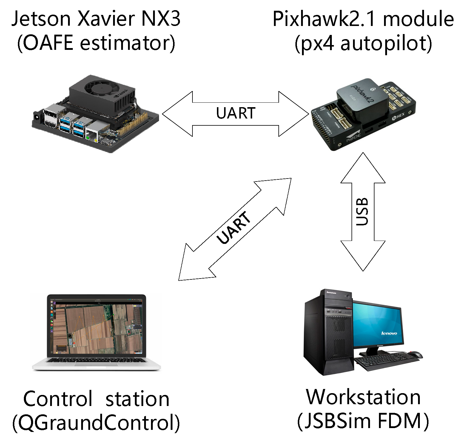
5.2. Hardware Modules

As shown in Figure 14, the Sula89 is equipped with a Pixhawk2.1 autopilot (running px4 v1.8.0) that facilitates automatic flight control, and an NVIDIA Jetson Xavier NX3 that runs the OAFE. The decision not to integrate the OAFE with the EKF module in px4 was made to maintain the original navigation module, thereby ensuring flight safety, and minimizing dimensionality and computational burden on the estimator. The data used in this study were collected by the Pixhawk2.1, which was connected with a CUAV digital airspeed and pitot tube, as well as a HEX Here3, which provided satellite positioning information.

The IMU cube of the Pixhawk 2.1 was replaced with the 6-axis IMU (BMI160), as well as the STMicroelectronics 3-axis magnetometer LIS3MDL. The BMI160 is a 6-axis IMU consisting of a digital, tri-axial, 16-bit acceleration sensor and a tri-axial 16-bit gyroscope.

Table 3 in Section 4 illustrates the sensor data that can be obtained from the hardware modules. [$\varphi ,\theta ,\psi$] were estimated based on the fusion of IMU, magnetometer and GPS data with high accuracy [38]. The sensor data and estimated [$\varphi ,\theta ,\psi$] transmitted from px4 to NX3 were downsampled to 50 Hz. In the flight test conducted for this study, the Sula89 was not equipped with an air data system or a flow angle sensor.

5.3. Field Test Setup

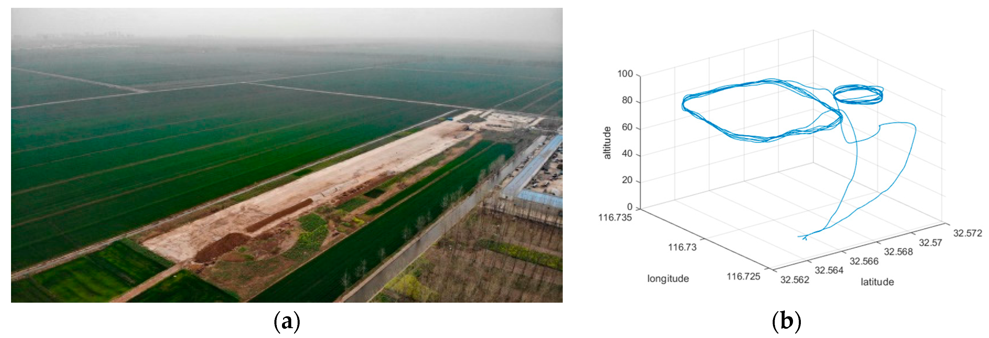
In 2024, a field flight verification of the OAFE was conducted in Anhui Province, China, at a standard airplane flight field with legal airspace. The site is located on a huge farm, as indicated in Figure 15. The local temperature was 17 °C, and the weather was overcast with a level 2 east wind (about 3 m/s).

In the flight test, the initialization of the OAFE was consistent with the simulation, as in Section 4.1.

First, the structure and electrical components of the Sula89a were checked. Then, the SUAV took off remotely in stabilized mode, and subsequently switched to mission mode to fly autonomously along a preset four-sided route (shown in Figure 15). Finally, the SUAV was remotely controlled to land, after which the data stored onboard were archived. The specific control parameters of the px4 employed in this test can be found in [39].

5.4. Results and Analysis

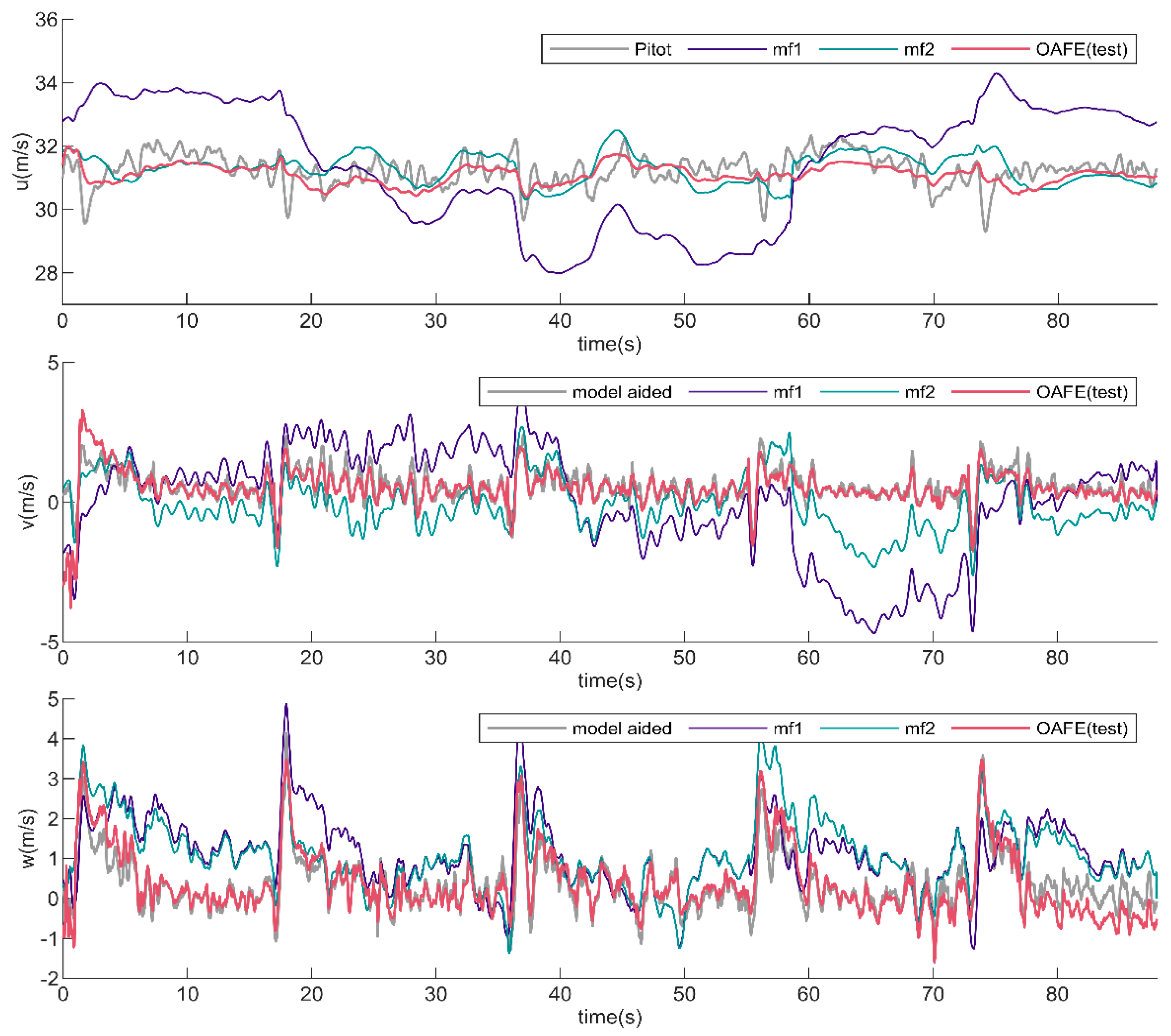
The estimated $\left[u,v,w\right]$ obtained from the OAFE method were compared with the reference, as depicted in Figure 16. The model-free-1 method, which is kinematic-based and assumes no wind (${\mathit{v}}_w^n=0$), is labeled with “mf1” in the figures below [16]. The model-free-2 method, with the assumption of $\beta =0$ and 2D horizontal wind, is labeled with “mf2” [15]. These two methods were selected based on the principle of immediate availability, like the OAFE. That is, there is no need for direct flow angle measurements, the prior acquisition of aerodynamic parameters, or pre-training.

The pitot airspeed is labeled “Pitot”. The ${\mathit{v}}_r^b$ estimated based on the model-aided method is labeled as “model-aided” and was used as the reference. Consistent with the approach outlined in [25], we also utilized the pre-identified aerodynamic parameters of the Sula89 [39].

As shown in Figure 16, the mf1 method presents the largest error for the estimation of $\left[u,v,w\right]$. The error of $u$ exhibits periodic oscillations due to the Sula89 flying a quadrilateral course in the wind field. The mf2 method shows significantly improved accuracy in estimating $u$, but not in estimating $v$ and $w$. The OAFE method consistently shows good agreement with the reference values for the estimation of $[u, v, w]$ throughout the entire flight. The $u$ estimated by OAFE is a fusion of inertial and differential pressure information, which is smoother than the reference $u_p$. We think that it is a beneficial effect, as $u$ is a long-term state and changes slowly.

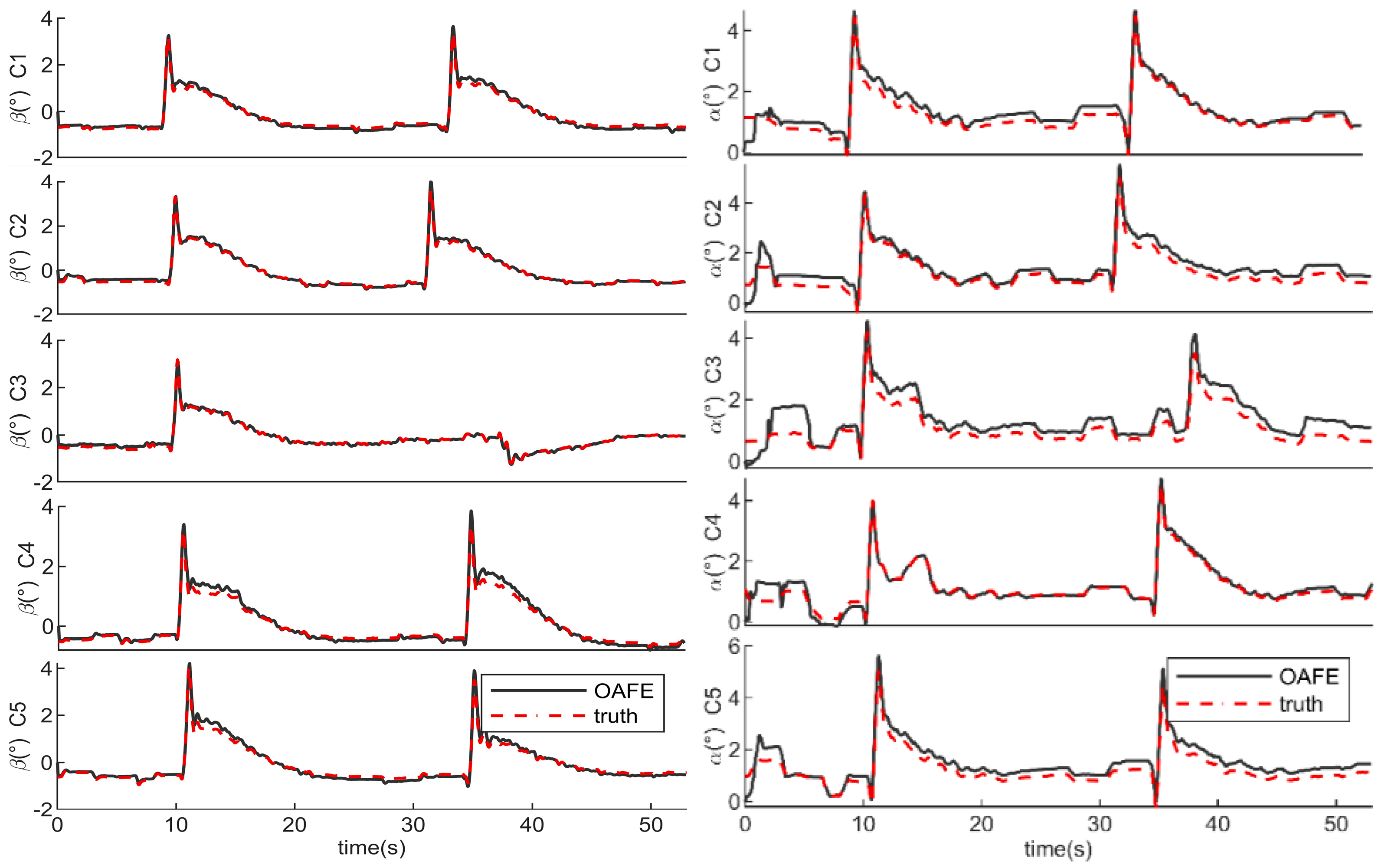
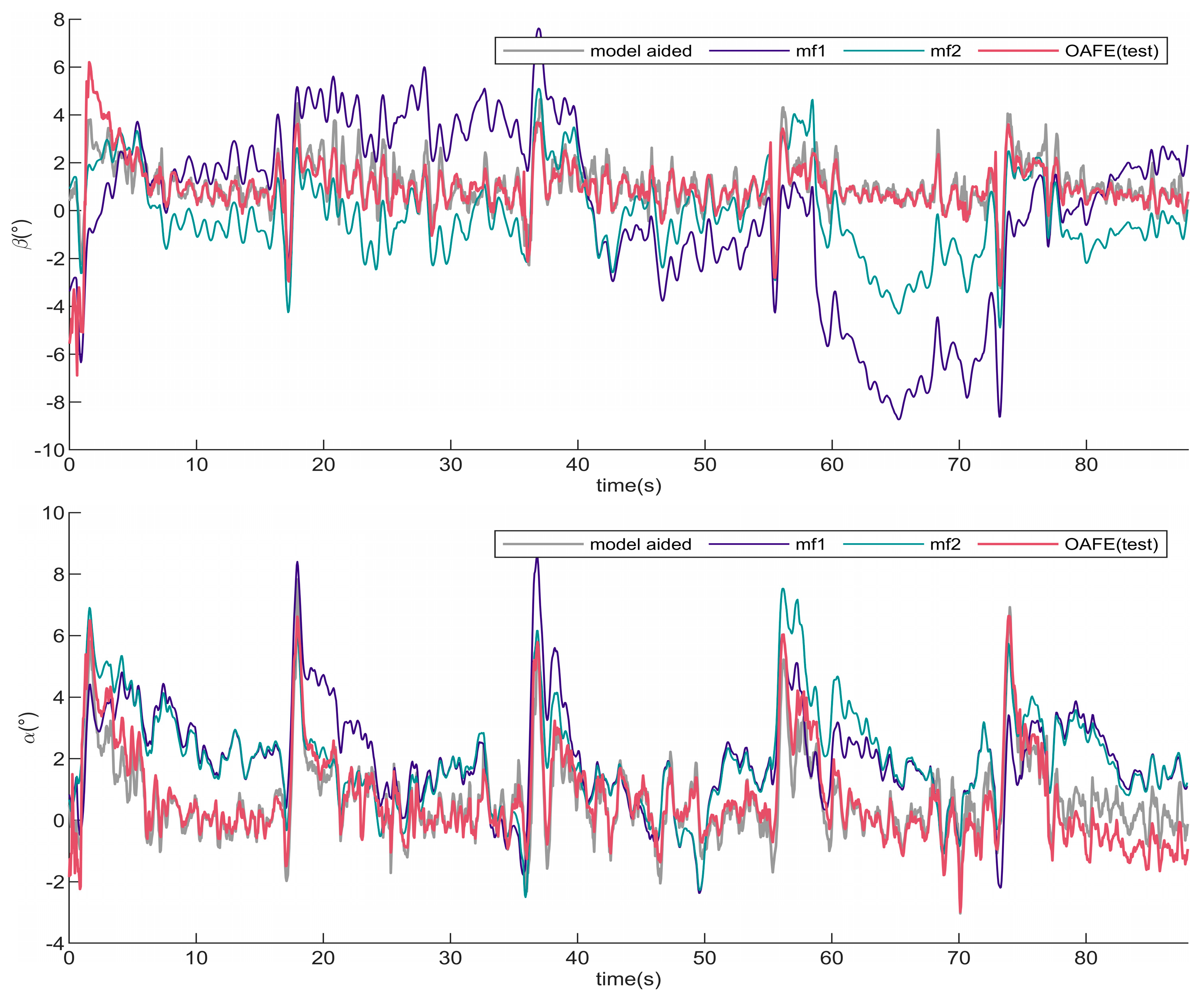
The flow angle $\left[\alpha , \beta \right]$, calculated from the estimated $\left[u,v,w\right]$, is shown in Figure 17.

Taking the results obtained from the “model-aided” method as a reference, the statistical performance of estimated $\left[v,w\right]$ and $\left[\alpha , \beta \right]$ are summarized in

Table 8. RMSE of estimates from different methods.

Estimates	$\mathit{v}$ (m/s)	$\mathit{w}$ (m/s)	$\mathit{\beta }$ (°)	$\mathit{\alpha }$ (°)
mf1	1.920	1.062	3.581	1.909
mf2	0.987	1.001	1.830	1.837
OAFE	0.407	0.324	0.748	0.593

.

Regarding the mf1 method, under the assumption of no wind, even with $v$, $w$ errors as low as 1–2 m/s, the method resulted in a significant flow angle error for the test SUAV. The error of $\beta$ even reached 10° at 65 s, presumably due to gusts of wind. This is to be expected since this method is designed for high-speed general aviation airplanes. As for the mf2 method, the estimated $v$ and $\beta$ fluctuated around zero, respectively, because it utilized $\beta$ = 0 as a measurement. Although its assumptions reduced the RMSE of $v$ and $\beta$, it did not lead to accurate estimates. For the estimation of $\alpha$, the improvement in mf2 over mf1 was very small.

The OAFE method significantly improved the estimation accuracy of $\beta$ and $\alpha$. Throughout the process, the OAFE estimates fit the reference values better and captured more nuanced dynamical changes. The estimation results of both $\beta$ and $\alpha$ are close to the accuracy limits of the reference ($1°$ and $0.5°$). Even though the lateral aerodynamics adopt only a “$\beta -C_Y$” model, the OAFE still demonstrated good accuracy in estimating $\beta$. This is attributed to the OAFE’s ability to capture the rapid changes in $\beta$ by fusing inertial data, even without incorporating aileron inputs, roll rates, or yaw rates into its aerodynamic model.

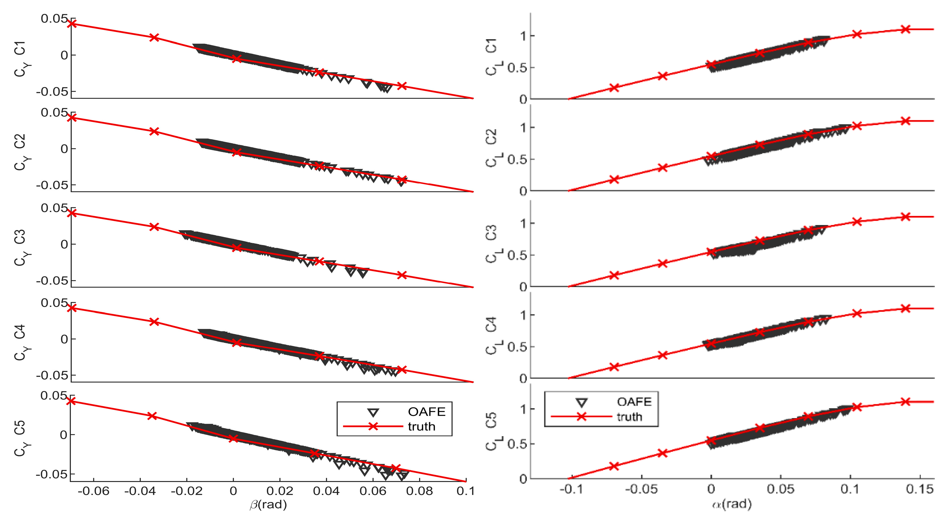
The distribution of estimation errors in the $\alpha$ domain is illustrated in Figure 18, revealing an increase in error with the increase in $\alpha$. This may be attributed to the fact that the OAFE method utilizes a “$L-\alpha$” linear model, while the tested SUAV’s “$L-\alpha$” curve has some anticipated nonlinear characteristics.

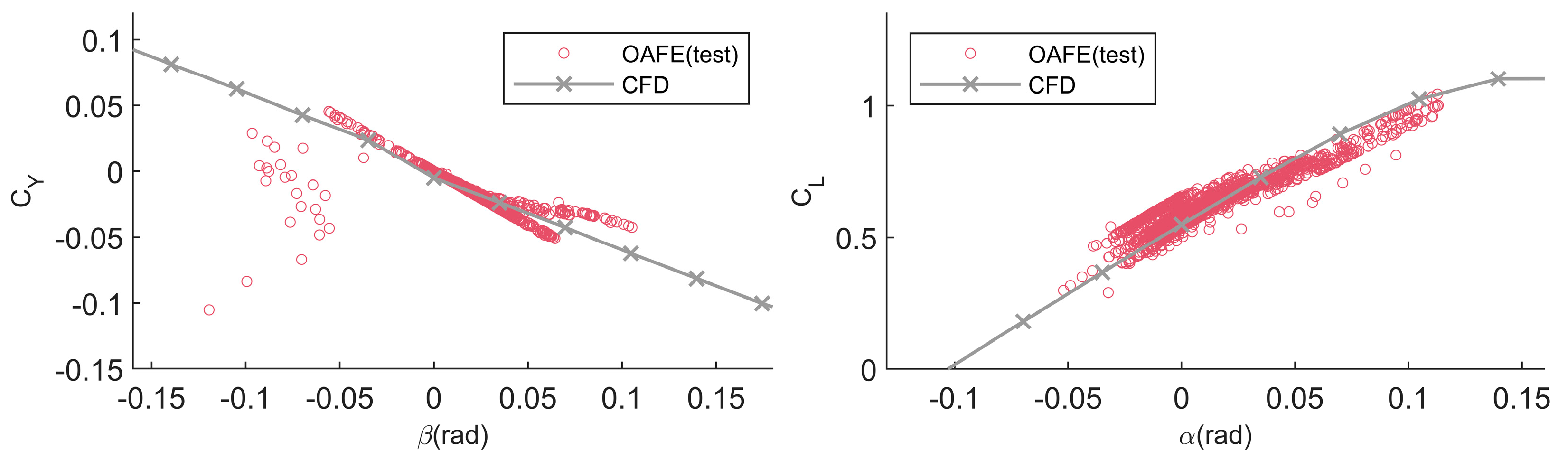
The estimated $C_Y,C_L$ by the OAFE are presented in Figure 19. The coefficients obtained from the CFD work were used as a reference and labeled as “CFD”. Among these, the lift coefficient $C_L$ showed a more obvious hysteresis in the interval of $\alpha =\left[\mathrm{0.05,0.12}\right]$.

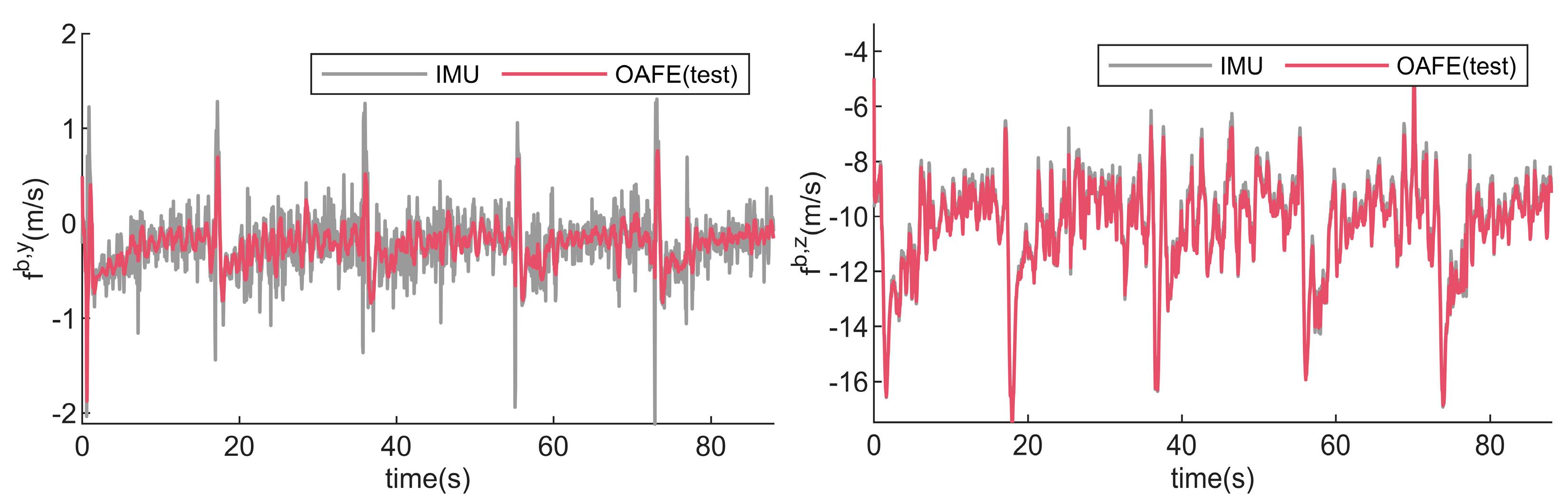
The estimated ${\mathit{f}}^{b,y}$ and ${\mathit{f}}^{b,z}$, derived from the estimated ${\mathit{v}}_r^b$ and estimated $\left[{C_L}_0,{C_L}_{\alpha },C_{L_q},C_{L_{{\delta }_e}},C_{Y_{\beta }}\right]$, are depicted in Figure 20. The measurement components from the IMU serve as the reference for comparison.

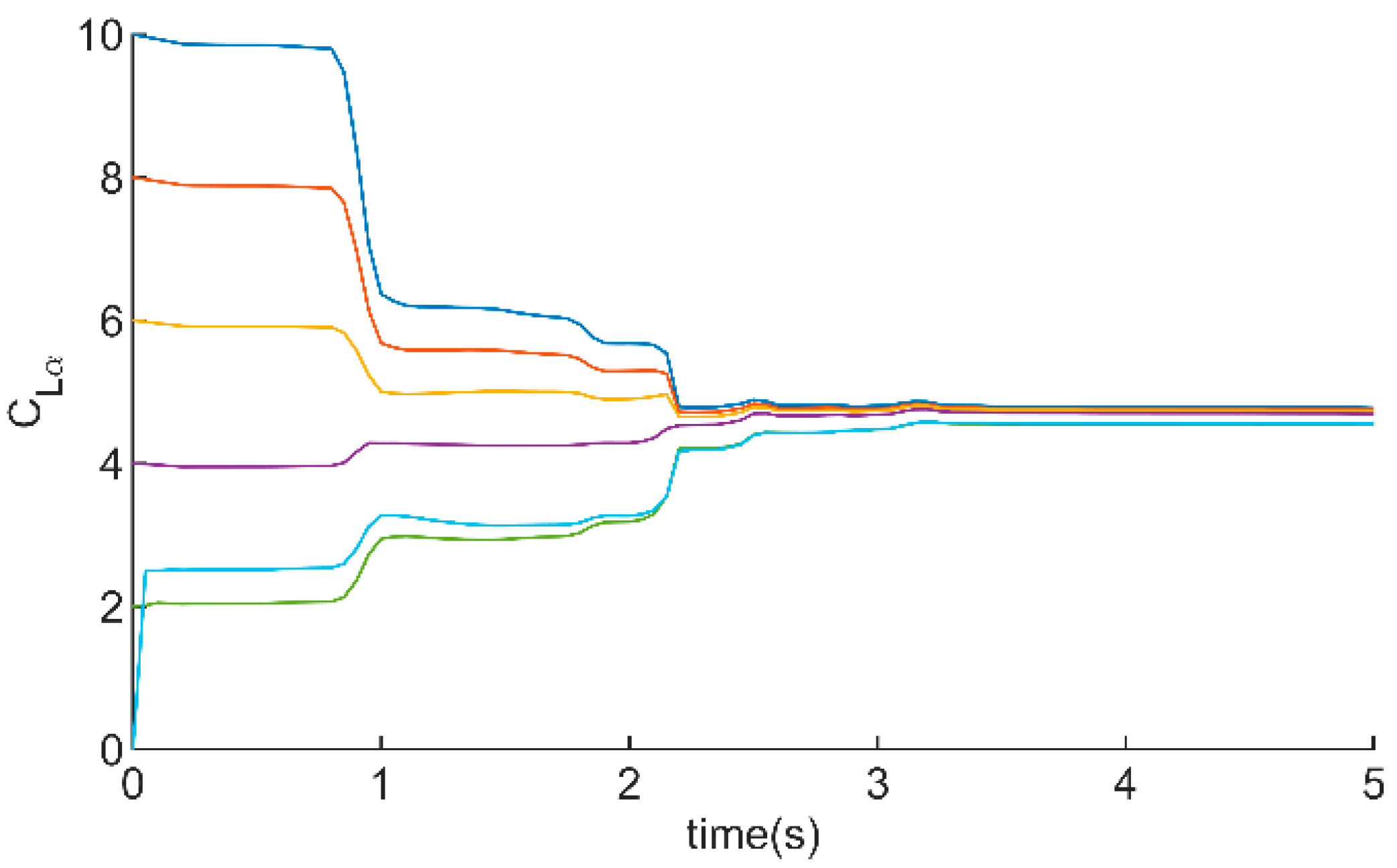
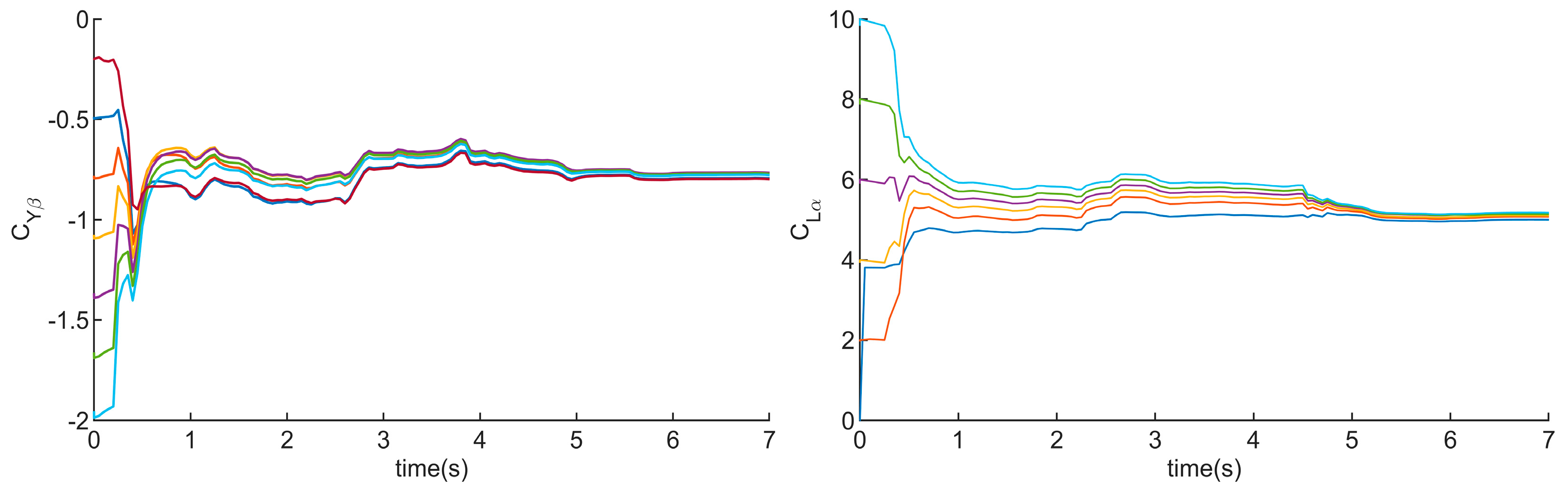
For further analysis, the original sensor data stored in the TF memory card were utilized for offline validation. As shown in Figure 21, the results indicate that $\left[C_{Y_{\beta }},C_{L_{\alpha }}\right]$ converge rapidly when different initial values are set. The amplitude of $C_{Y_{\beta }}$ reduces to 7% after 3 s. Similarly, the amplitude of $C_{L_{\alpha }}$ decreases to 5% after 3 s.

6. Conclusions

An OAFE method that yields flow angle estimates of SUAVs solely using a standard sensor suite is proposed in this study. The OAFE’s filter loop utilizes inertial data and incorporates noisy aerodynamic derivatives identified online to refine its performance. The noisy aerodynamic derivatives are generated in real time by the optimizer loop of the OAFE in the absence of flow angle measurements. The optimizer approximately determines these derivatives based on multi-period sensor data, motion-continuity rules, and aerodynamics.

The OAFE method was evaluated through simulations and field tests. The simulation results revealed that the estimated $\alpha$ and $\beta$ displayed an RMSE of approximately $0.11°$ and $0.24°$, respectively. In field flight tests, the results indicated an RMSE of 0.75° for $\beta$ and 0.59° for $\alpha$, which fell within the error range of the reference method.

The OAFE method does not require flow angle measurements or the prior acquisition of aerodynamic parameters (derivatives or neural networks). Therefore, it is economical and does not require identification or training efforts in advance, making it suitable for quick deployment on different SUAVs and adaptable to changes in aerodynamic parameters caused by icing or other factors.

Further efforts will be dedicated to completing the estimation of other key aerodynamic derivatives without the need for α and β measurements. In addition, the OAFE will be utilized for the estimation of complete-state air data.