Physics-Informed Neural Networks for Unmanned Aerial Vehicle System Estimation

Abstract

The dynamic nature of quadrotor flight introduces significant uncertainty in system parameters, such as thrust and drag factors. Consequently, operators grapple with escalating challenges in implementing real-time control actions. This study presents an approach for estimating the dynamic model of Unmanned Aerial Vehicles based on Physics-Informed Neural Networks (PINNs), which is of paramount importance due to the presence of uncertain data and since control actions are required in very short computation times. In this regard, by including physical laws into neural networks, PINNs offer the potential to tackle several issues, such as heightened non-linearities in low-inertia systems, elevated measurement noise, and constraints on data availability or uncertainties, while ensuring the robustness of the solution, thus ensuring effective results in short time, once the network training has been performed and without the need to be retrained. The effectiveness of the proposed method is showcased in a simulation environment with real data and juxtaposed with a state-of-the-art technique, such as the Extended Kalman Filter (EKF). The results show that the proposed estimator outperforms the EKF both in terms of the efficacy of the solution and computation time.

1. Introduction

1.1. Context

One of the biggest hurdles in control theory is creating a dynamic model of a physical system to understand and forecast its future behavior. This can result in a very complicated mathematical representation of the system, often necessitating specific experiments to estimate unknown parameters (see Ref. [1]). This is especially true for complex systems like Unmanned Aerial Vehicles (UAVs), which are inherently unstable and have multiple inputs and outputs (MIMO). When real-world data are unavailable (due to a lack of reliable system knowledge or inaccurate measurements), system identification offers an effective solution. This technique involves deriving mathematical models of a dynamic system from measured input and output data. Two approaches can be adopted for system identification, namely, grey box model, also known as the semi-physical model (i.e., when the constructed model still has a number of unknown free parameters that are estimated through system identification) and the black box model (i.e., when no prior model is available) Ref. [2]. Regardless of the adopted model, system identification strategies consist of designing and conducting an identification experiment to collect data, selecting the structure of the dynamic system and specifying which parameters are to be identified, and fitting the model parameters to the obtained data; the overall quality of the resulting model is then evaluated through a validation procedure Ref. [1].

Research on system identification has garnered considerable attention in recent decades, starting from the 1950s, and has become a vital discipline in various applications within the field of automatic control. This includes areas such as robotics, industrial processes, reduced-order modeling, and model testing.

In recent decades, as researchers and engineers have gained access to larger numbers of data, one of the most widely used methods for system identification has been the Least Squares Method. This approach can be considered the foundation of data-driven system modeling.

In Ref. [3], a classification of model identification is presented based on the applied methodologies. The classification includes Fuzzy Logic Theory, Genetic Algorithm, Neural Network, Swarm Intelligence Optimization Algorithms, Auxiliary Model Identification Method, Hierarchical Method, and Stochastic Theory Ref. [4].

Referring to the last method, in Ref. [5] crucial principles of realization theory were introduced, particularly emphasizing controllability and observability concepts. Their focus was on linear system identification, with a special emphasis on establishing the minimal state-space representation to define the subspace within which the system dynamics evolves. They pioneered the concept of state-variable equations, which facilitates the realization of an external description through an equivalent internal description of a dynamical system. A second algorithm addressing the same problem was simultaneously presented by Kalman (see Ref. [6]), utilizing the principles of controllability and observability and necessitating linear algebra-type computations. State-space models are particularly well-suited for this approach as they lend themselves to linear algebra techniques, robust numerical simulation, and modern control design methods. A few years later, Ho and Kalman Ref. [5] approached the same problem from a new perspective. They demonstrated that the minimum realization problem is equivalent to a representation problem involving a sequence of real matrices known as Markov parameters (pulse response samples).

During the 1990s, expanding upon the foundational work by Gilbert and Kalman, various methods were developed to identify the most observable and controllable subspace of a system based on given input–output (I/O) data. Some years later, at NASA, Juang devised an approach to concurrently ascertain a linear state-space model and the corresponding Kalman filter using noisy input–output measurements (see Ref. [7] for details). Referred to as the Observer/Kalman Identification Algorithm (OKID) and exclusively formulated in the time domain, this method computes the Markov parameters of a linear system. Subsequently, both the state-space model and a corresponding observer are determined simultaneously from these parameters. The Kalman Filter was therefore a reference point for identification in the case of linear systems and its parameters. Subsequently, the theory was extended to nonlinear systems through the Extended Kalman Filter (EKF) in various versions (see, e.g., the work in Ref. [8] for the polynomial one), starting from a series of measurements subject to noise, and was successful in any application that could be linked to control theory.

In this regard, it is worth noting that an interesting comparison among modern methods for the parameter estimation of aircrafts is presented in Ref. [9]. In particular, by using real flight data, the authors find that the performance of Filter Error Methods (FEMs), such as Extended Kalman Filter (EKF) and Unscented Kalman Filter (UKF), prevail over Equation Error Methods (EEMs) and Output Error Methods (OEMs), particularly in the presence of turbulence and noise.

In recent times, machine learning techniques, especially artificial neural networks, have gained prominence in addressing control problems. Neural networks, which have evolved significantly since the late 20th century, have found applications in diverse fields, particularly cyber-physical systems. They are especially useful in intelligent control, nonlinear optimization, computer vision, biomedical engineering, robotics, and system identification. Neural network identification exploits the nonlinear structure of a system, allowing it to simulate input–output relationships by approximating any nonlinear mapping. It employs the self-adaptation and self-learning capabilities of neural networks to implement simple learning algorithms in engineering, ultimately achieving the forward or inverse model of the system through training. This method exhibits the following characteristics:

• No need to establish the model structure of the actual system, as the neural network itself serves as a model for network identification.
• It is capable of identifying any linear or nonlinear model.
• The neural network not only serves as a model but is also an actual system achievable through physics.

However, it comes with certain limitations:

• The local minimum problem.
• Lengthy training time and slow learning speed.
• Difficulty in extracting ideal training samples.
• Challenges in optimizing the network structure.
• Difficulty in completely solving the convergence problem theoretically for the neural network algorithm.

To address these limitations, numerous researchers have proposed improved neural network identification methods, resulting in favorable identification outcomes (see, e.g., Refs. [10,11]).

1.2. Relevant and Related Work

In the above-described context, the main contribution of this paper is to exploit the power in the management and use of a limited number of data available data in Neural Networks with the physical laws of the flight dynamics of a quadcopter. In particular, we use Physics-Informed Neural Networks (PINNs), also known as Theory-Trained Neural Networks, to estimate the drone model. In fact, in the last decade, aerial robots, and particularly small UAVs and drones, have witnessed continuously increasing use in a wide range of services (see, e.g., Ref. [12]). As a consequence, the identification and control (and hence the system parameters estimation) of these systems is of paramount importance from different point of view (see Refs. [13,14]).

We conclude this section by highlighting that the use of PINNs for system identification has been attracting attention in the research community. As an example, the work in Ref. [15] proposes the use of PINNs for non-linear system identification for power system dynamics. In particular, the final aim of this contribution is to discover the frequency dynamics of future power systems. To assess the performance of the presented model and validate their proposal, the authors compare the estimator against the UKF. PINNS are also used in Ref. [16] to discover the ordinary differential equation (ODE) of a rotor system from noise measurements and assess the healthy/faulty machine condition. The validation is performed on a test bench. The system identification of structural systems with a multiphysics damping model through PINNs is presented in Ref. [17], while in Ref. [18] it is adopted to estimate motion and identify the system parameters of a moored buoy under different sea states. In Ref. [19] it is applied to the understanding of the dynamics of COVID-19. The authors of Ref. [20] demonstrate the utilization of Pontryagin Neural Networks (PoNNs) to acquire control strategies for achieving fuel-optimal trajectories. PoNNs, a subtype of Physics-Informed Neural Network (PINN), are tailored for solving optimal control problems through indirect methods. In Ref. [21], Physics-Informed Neural Networks are used to examine the mechanical properties of a helicopter blade. The work Ref. [22] proposes a novel nonlinear Model Predictive Control approach, informed by Physics-Informed Neural Networks, to optimize the trajectory tracking of Automated Guided Vehicles in intricate dynamic environments. In Ref. [23], the PennyLane quantum device simulator is utilized to investigate the application of quantum and hybrid quantum-classical Physics-Informed Neural Networks to the solution of both transient and steady-state partial differential equations in one and two spatial dimensions.

In Ref. [24], a Nonlinear AutoRegressive with eXogenous inputs (NARX) network with a serial-parallel structure was employed to identify an unknown aerial delivery system equipped with a ram-air parachute. The dataset was generated using the software-in-the-loop simulation method. Gazebo served as the simulator, while PX4 was utilized as the autopilot software. The authors of Ref. [25] investigate the strengths of Legendre multiwavelet (LW) bases to develop a Legendre multiwavelet neural network (LWNN). This network has a straightforward structure comprising an input layer, a hidden layer, and an output layer. Notably, the activation functions in the hidden layer are based on LW bases. This choice is motivated by the rich properties of LW bases, including piecewise polynomial nature, orthogonality, and various regularities. These properties empower LWNNs to excel in approximating complex characteristics, such as uncertainties, step functions, nonlinearities, and ramps, in dynamical systems, surpassing traditional wavelet neural networks. The authors of Ref. [26] present a physics-based identification method employing genetic algorithms. The primary goal is to determine a parametric matrix, designated as A, that characterizes the time-invariant linear model representing the longitudinal dynamics of an aircraft. This is accomplished by introducing a fitness function rooted in the properties of the transition matrix and capitalizing on the strengths of the genetic algorithm, particularly its ability to constrain the search ranges of unknown parameters. These unknown parameters are associated with the specific aircraft type and flight conditions considered during the identification process.

1.3. Original Contributions and Organization

Different types of studies have been conducted in the drone and aircraft sector in general for the estimation of the system and/or parameters with many methods, including those that use neural networks with different architectures or combined with specific algorithms. To the best of our knowledge, the first attempt to apply PINNs to quadrotor dynamical modeling is presented in Ref. [27]. This study compares PINNs with other existing methods, demonstrating superior performance in terms of test error and the ability to uncover underlying relationships between parameters compared to linearized mathematical models and classical black-box DNN approaches. While Ref. [27] focuses on orientation estimation, our work addresses all state variables, including spatial ones. By avoiding linearized models, we aim to leverage the power of neural networks and the physical model to identify nonlinearities. This preliminary research seeks to optimize the weighting of neural networks and the physical model as data availability varies. Future research, detailed in the conclusions, will further explore this direction. The reminder of the paper is organized as follows. In Section 2, the drone dynamics model is recalled. Section 3 illustrates the two methodologies chosen to compare system model identification: a quick recall of the Extended Kalman Filter, and then the idea on which PINNs are based is described. Section 4 shows the simulation and comparison results between the methods mentioned above. Some final considerations and future research ideas conclude the paper.

2. Mathematical Model of a Quadrotor

The quadrotor analyzed in this study is composed of a rigid structure with four rotors (for more details, refer to [28,29]). The propellers produce a force $F_i=b·{\omega }_{p,i}^2$, which is proportional to their angular velocity ${\omega }_{p,i}$, for $i=1,2,3,4$. Propellers 1 and 3 spin counterclockwise, while propellers 2 and 4 spin clockwise. In the following discussion, the quadrotor’s orientation will be described using Euler angles. The frames $RC(O,e_1,e_2,e_3)$ and $R\Gamma (\Omega ,{\epsilon }_1,{\epsilon }_2,{\epsilon }_3)$) represent the reference systems fixed to the Earth and the quadrotor, respectively, with $\Omega$ located at the quadrotor’s center of mass (see Figure 1).

The quadrotor’s position in $RC$ is represented by $p={(x,y,z)}^T$, while its orientation is defined by the Euler angles $\alpha ={(\varphi ,\theta ,\psi )}^T$, where $\varphi \in [-\pi /2,\pi /2)$, $\theta \in (-\pi /2,\pi /2)$, and $\psi \in [-\pi ,\pi )$ correspond to the roll, pitch, and yaw angles, respectively. The 3–2–1 sequence is utilized here, as in [30]. Furthermore, $v={(v_x,v_y,v_z)}^T$ and $\omega ={({\omega }_1,{\omega }_2,{\omega }_3)}^T$ denote the linear and angular velocities of the quadrotor’s center of mass, expressed in $RC$ and $R\Gamma$, respectively. The quadrotor’s translational dynamics are expressed in $RC$, while its rotational dynamics are expressed in $R\Gamma$:

$$\begin{array}{cc}\hfill \dot{p}& =v\hfill \\ \hfill \dot{v}& ={\displaystyle \frac{1}{m}}\left(f_p+f_g\right)\hfill \\ \hfill \dot{\alpha }& =M\left(\alpha \right)\omega \hfill \\ \hfill \dot{\omega }& =J^{-1}\left(-\tilde{\omega }J\omega +{\tau }_p+{\tau }_{gy}\right)\hfill \end{array}$$

(1)

where m represents the mass of the quadrotor, $f_p=\mathcal{R}\left(\alpha \right){\phi }_p$ is the force exerted by the propellers in $RC$ (${\phi }_p$ is the same force, but expressed in $R\Gamma$), J (a positive definite symmetric matrix in ${\mathbb{R}}^{3\times 3}$, expressed in $R\Gamma$) is the quadrotor’s inertia matrix, and

$$\tilde{\omega }=\left(\begin{array}{ccc}0& -{\omega }_3& {\omega }_2\\ {\omega }_3& 0& -{\omega }_1\\ -{\omega }_2& {\omega }_1& 0\end{array}\right)$$

(2)

is the so-called dyadic representation of $\omega$ (see [14] for more details). Furthermore,

$${\phi }_p=\left(\begin{array}{c}0\\ 0\\ u_p\end{array}\right),u_p=\sum _{i=1}^4{F}_i,f_g=\left(\begin{array}{c}0\\ 0\\ -mg\end{array}\right)$$

(3)

$${\tau }_p=\left(\begin{array}{c}{\tau }_1\\ {\tau }_2\\ {\tau }_3\end{array}\right)=\left(\begin{array}{c}\ell b({\omega }_{p,2}^2-{\omega }_{p,4}^2)\\ \ell b({\omega }_{p,3}^2-{\omega }_{p,1}^2)\\ c({\omega }_{p,1}^2-{\omega }_{p,2}^2+{\omega }_{p,3}^2-{\omega }_{p,4}^2)\end{array}\right)$$

(4)

are the input forces (as shown in (3)) and moments (as shown in (4)) generated by the propellers (expressed in $R\Gamma$), where ℓ is the distance from the center of mass $CG$ to the rotor shaft, and b (with units [b] = ${\displaystyle \frac{N,s^2}{ra{d}^2}}$) and c (with units [c] = ${\displaystyle \frac{N,s^2,m}{ra{d}^2}}$) are the thrust and drag coefficients, respectively. It is evident that:

$$\begin{array}{l}\left(\begin{array}{c}{F}_1\\ F_2\\ F_3\\ F_4\end{array}\right)={\left(\begin{array}{cccc}1& 1& 1& 1\\ 0& \ell & 0& -\ell \\ -\ell & 0& \ell & 0\\ c& -c& c& -c\end{array}\right)}^{-1}\left(\begin{array}{c}{u}_p\\ {\tau }_1\\ {\tau }_2\\ {\tau }_3\end{array}\right),\\ \left(\begin{array}{c}{\omega }_{p,1}^2\\ {\omega }_{p,2}^2\\ {\omega }_{p,3}^2\\ {\omega }_{p,4}^2\end{array}\right)=\left(\begin{array}{cccc}\frac{1}{4b}& 0& \frac{-1}{2b\ell }& \frac{1}{4c}\\ \frac{1}{4b}& \frac{1}{2b\ell }& 0& \frac{-1}{4c}\\ \frac{1}{4b}& 0& \frac{1}{2b\ell }& \frac{1}{4c}\\ \frac{1}{4b}& \frac{-1}{2b\ell }& 0& \frac{-1}{4c}\end{array}\right)\left(\begin{array}{c}{u}_p\\ {\tau }_1\\ {\tau }_2\\ {\tau }_3\end{array}\right),\end{array}$$

(5)

$${\omega }_{p,i}=\sqrt{{\displaystyle \frac{F_i}{b}}},0\le F_i\le F_{i,max},0\le {\omega }_{p,i}\le {\omega }_{p,i,max}$$

with $i=1,2,3,4$, where $F_{i,max}$ and ${\omega }_{p,i,max}$ represent the maximum forces and angular velocities for each propeller, constrained by physical limitations. Additionally, $f_g$ in (3) refers to the gravitational force, expressed in $RC$. Vectors expressed in $R\Gamma$ are converted into vectors in $RC$ using the rotation matrix

$$R(\alpha )=\left(\begin{array}{ccc}{c}_{\theta }{c}_{\psi }& s_{\varphi }{s}_{\theta }{c}_{\psi }-c_{\varphi }{s}_{\psi }& c_{\varphi }{s}_{\theta }{c}_{\psi }+s_{\varphi }{s}_{\psi }\\ c_{\theta }{s}_{\psi }& s_{\varphi }{s}_{\theta }{s}_{\psi }+c_{\varphi }{c}_{\psi }& c_{\varphi }{s}_{\theta }{s}_{\psi }-s_{\varphi }{c}_{\psi }\\ -s_{\theta }& s_{\varphi }{c}_{\theta }& c_{\varphi }{c}_{\theta }\end{array}\right)$$

(6)

where $c_{★}=cos(★)$, $s_{★}=sin(★)$, $★=\varphi ,\theta ,\psi$. The angular velocity dynamics are expressed using the following matrix:

$$M(\alpha )=\left(\begin{array}{ccc}1& s_{\varphi }{\mathrm{t}\mathrm{g}}_{\theta }& c_{\varphi }{\mathrm{t}\mathrm{g}}_{\theta }\\ 0& c_{\varphi }& -s_{\varphi }\\ 0& s_{\varphi }{\mathrm{s}\mathrm{c}}_{\theta }& c_{\varphi }{\mathrm{s}\mathrm{c}}_{\theta }\end{array}\right)$$

where ${\mathrm{tg}}_{★}=tan(★)$ and ${\mathrm{sc}}_{★}=sec(★)$ with $★=\varphi ,\theta ,\psi$. Assuming small angles for $\varphi$ (roll) and $\theta$ (pitch), which is reasonable for a quadrotor performing non-aggressive maneuvers, this matrix can be approximated by the identity matrix, i.e., $M\left(\alpha \right)\simeq I_{3x3}$[31]. Therolling torque ${\tau }_1$ is generated by the forces $F_2$ and $F_4$, while the pitching torque ${\tau }_2$ is generated by the forces $F_1$ and $F_3$. According to Newton’s third law, the propellers exert a yawing torque ${\tau }_3$ on the quadrotor body in the direction opposite to the propeller rotation. Furthermore, the gyroscopic torque arising from the propeller rotations is given by

$${\tau }_{gy}=\sum _{i=1}^4{(-1)}^i{J}_{p,i}{\omega }_{p,i}\tilde{\omega }{ϵ}_3$$

(7)

where $J_{p,i}$, for $i=1,2,3,4$, represents the moment of inertia of the $i_{\mathrm{th}}$ motor and propeller about its axis of rotation. Finally, the gyroscopic torque can also be expressed as

$${\tau }_{gy}^{\circ }=\sum _{i=1}^4{(-1)}^i{J}_p^{\circ }{\omega }_{p,i}\tilde{\omega }{ϵ}_3=J_p^{\circ }{\omega }_p\left(\begin{array}{c}{\omega }_2\\ -{\omega }_1\\ 0\end{array}\right)$$

(8)

where ${\omega }_p=-{\omega }_{p,1}+{\omega }_{p,2}-{\omega }_{p,3}+{\omega }_{p,4}$ is referred to as the rotor relative speed. Given these conditions, the mathematical model (1) of the quadrotor can be rewritten as:

$$\begin{array}{cc}\hfill \dot{x}\left(t\right)& =v_x\left(t\right),\dot{y}\left(t\right)=v_y\left(t\right),\dot{z}\left(t\right)=v_z\left(t\right)\hfill \\ \hfill {\dot{v}}_x\left(t\right)& =\left(c_{\varphi \left(t\right)}{s}_{\theta \left(t\right)}{c}_{\psi \left(t\right)}+s_{\varphi \left(t\right)}{s}_{\psi \left(t\right)}\right){\displaystyle \frac{u_p\left(t\right)}{m}}\hfill \\ \hfill {\dot{v}}_y\left(t\right)& =\left(c_{\varphi \left(t\right)}{s}_{\theta \left(t\right)}{s}_{\psi \left(t\right)}-s_{\varphi \left(t\right)}{c}_{\psi \left(t\right)}\right){\displaystyle \frac{u_p\left(t\right)}{m}}\hfill \\ \hfill {\dot{v}}_z\left(t\right)& =-g+c_{\varphi \left(t\right)}{c}_{\theta \left(t\right)}{\displaystyle \frac{u_p\left(t\right)}{m}}\hfill \\ \hfill \dot{\varphi }\left(t\right)& ={\omega }_1\left(t\right),\dot{\theta }\left(t\right)={\omega }_2\left(t\right),\dot{\psi }\left(t\right)={\omega }_3\left(t\right)\hfill \\ \hfill {\dot{\omega }}_1\left(t\right)& ={\displaystyle \frac{J_2-J_3}{J_1}}{\omega }_2\left(t\right){\omega }_3\left(t\right)+{\displaystyle \frac{J_p}{J_1}}{\omega }_p\left(t\right){\omega }_2\left(t\right)+{\displaystyle \frac{1}{J_1}}{\tau }_1\left(t\right)\hfill \\ \hfill {\dot{\omega }}_2\left(t\right)& ={\displaystyle \frac{J_3-J_1}{J_2}}{\omega }_1\left(t\right){\omega }_3\left(t\right)-{\displaystyle \frac{J_p}{J_2}}{\omega }_p\left(t\right){\omega }_1\left(t\right)+{\displaystyle \frac{1}{J_2}}{\tau }_2\left(t\right)\hfill \\ \hfill {\dot{\omega }}_3\left(t\right)& ={\displaystyle \frac{J_1-J_2}{J_3}}{\omega }_1\left(t\right){\omega }_2\left(t\right)+{\displaystyle \frac{1}{J_3}}{\tau }_3\left(t\right).\hfill \end{array}$$

(9)

where the state space vector is $\left[xyz{v}_x{v}_y{v}_z\varphi \theta \psi {\omega }_1{\omega }_2{\omega }_3\right]$, and the control input is $\left[u_p{\tau }_1{\tau }_2{\tau }_3\right]$. Given the aims of the research, it is assumed that we have a limited number of data available in the form input–output (state). Moreover, the system identification methods that will be presented in Section 3 are in discrete form. Thus, the quadrotor system Equations (9) will be implemented in discrete form by keeping the functions constant over each time interval $[t_i,t_{i+1})$, where $t_{i+1}-t_i=\Delta t$ for $i=0,\cdots ,i_{max}-1$, and $t_{i_{max}}=t_f$ represents the final mission time. This discrete-time formulation allows for accurate modeling within each interval, enhancing the overall performance of the UAV system. The digitalization is obtained by a first-order discretization.

3. System Identification Methods

3.1. Extended Kalman Filter

The EKF ([32]) is an adaptation of the standard Kalman filter designed for use when the system and/or measurement models are nonlinear. The approach underlying the extended Kalman filter is based on the following procedure. Given the system type:

$$\begin{array}{c}\hfill s_k=f(s_{k-1},{\mu }_{k-1})+n_{1,k}\\ \hfill z_k=h\left(x_k\right)+n_{2,k}\end{array}$$

(10)

where $s_k$ is the state space vector, $z_k$ is the output, and ${\mu }_{k-1}$ is the control input, it approximates the nonlinear functions of the system $x_k$ and $z_k$, through a Taylor series expansion stopped at the first order around the current estimate, thus making the system linear. The noise vectors $n_{1,k}$ and $n_{2,k}$ represent disturbances affecting the state and measurements, respectively, and are assumed to be uncorrelated with each other. Given a random variable s, we want to know the probability density of the variable y obtained from the transformation of the variable s. Moments up to first order are studied.

$$\begin{array}{c}\hfill s\sim N(\widehat{s},{\sigma }_s^2)=\widehat{s}+{\delta }_s\mathrm{with}{\delta }_s\sim N(0,{\sigma }_s^2)\end{array}$$

(11)

$$\begin{array}{c}\hfill y=f\left(s\right)=f(\widehat{s}+{\delta }_s)\end{array}$$

(12)

whose development is $y=f\left(\widehat{s}\right)+\lambda f{\delta }_s+{\displaystyle \frac{1}{2}}{\Delta }^{2}f{\delta }_s^2$. Then, $J_s^h={\left[{\displaystyle \frac{\partial h}{\partial s}}\right]}_{s={\widehat{s}}_{k|k}}$ is defined as the Jacobian matrix of the function h with respect to s and $J_s^f={\left[{\displaystyle \frac{\partial f}{\partial s}}\right]}_{s={\widehat{s}}_{k|k}}$ is the Jacobian matrix of f with respect to s. Moreover, the conditional probability function is assumed to be Gaussian. Using these approximations, the system turns out to be linear, so the Kalman filter can be applied, obtaining the following recursive equations (referring, respectively, to the prediction and the correction):

$$\begin{array}{c}\hfill {\widehat{s}}_{k|k-1}=f(s_{k|k-1},{\mu }_k)\\ \hfill P_{k|k-1}=J_s^f{P}_{k-1|k-1}{J}_s^{f^T}+Q\end{array}$$

(13)

$$\begin{array}{c}\hfill n_{2,k}=z_k-h\left({\widehat{s}}_{k|k-1}\right)\\ \hfill S_k=J_s^h{P}_{k|k-1}{J}_s^{h^T}+R_k\\ \hfill K_k=P_{k|k-1}{J}_s^{h^T}{S}_k^{-1}\\ \hfill s_{k|k}=s_{k|k-1}+K_k{n}_{2,k}\\ \hfill P_{k|k}=(I-K_k{J}_s^h)P_{k|k-1}\end{array}$$

(14)

where the matrices Q and R have the same properties as in the linear Kalman filter. However, there are no assurances regarding the quality of the estimates produced, and the extended Kalman filter is highly sensitive to the accuracy of the initial estimates (see [32]).

3.2. Physics-Informed Neural Networks

PINNs are introduced to integrate physical laws, typically described by Ordinary Differential Equations (ODEs), into Deep Neural Networks (DNNs) (see [33]). This approach trains DNNs in a supervised fashion to comply with given physical laws, enabling the automatic discovery of data-driven solutions for ODEs, as demonstrated in the application under consideration (Equation (9)). The core idea behind PINNs is to incorporate the differential equation into the loss function, as illustrated in Figure 2, enhancing the network’s robustness and facilitating accurate approximations even in data-scarce scenarios. In this study, we focus on parametrized and nonlinear partial differential equations in the general form:

$${\partial }_t\widehat{y}+N\left[\widehat{y};\lambda \right]=0.t\in \left[0,T\right]$$

(15)

where $\widehat{y}(t,x)$ represents the latent (hidden) solution or the state of the dynamic system, and $N\left[·\right]$ denotes a nonlinear differential operator parametrized by $\lambda$. We define $l(t,x)$ as the expression on the left-hand-side of Equation (15), i.e.,

$$l:=\partial \widehat{y}+N\left[\widehat{y}\right]$$

(16)

and then we continue by modeling $\widehat{y}(t,x)$ using a deep neural network. In this context, $\widehat{y}$ serves as the output of a layered architecture neural network, denoted by $l_w\left(t\right)$, where $\widehat{y}=l_w\left(t\right)$; let $l_w$ denote the mapping function learned by a deep network with adaptive weights w. In this context, the neural network is expected to learn the solution of a specified ODE as a function of continuous time t.

By using automatic differentiation and the chain rule, we can derive a neural network representing $\widehat{y}(t,x)$. Importantly, this network shares the same parameters as the one representing $\widehat{y}(t,x)$ but may employ different activation functions due to the influence of the differential operator N. Assuming an autonomous system, we train a neural network $\widehat{y}\left(t\right)$ by optimizing its shared parameters with those of $\widehat{y}(t,x)$ and $l(t,x)$. Our goal is to minimize a Mean Square Error (MSE) cost function.

$$MSE=MS{E}_{\widehat{y}}+\gamma MS{E}_l.$$

(17)

where:

$$MS{E}_{\widehat{y}}={\displaystyle \frac{1}{N_{\widehat{y}}}}\sum _{i=1}^{N_{\widehat{y}}}{\displaystyle \frac{1}{N_t}}\sum _{j=1}^{N_t}{|{\widehat{y}}_i\left(t^j\right)-{\widehat{y}}_{i,ref}^j|}^2$$

(18)

$$MS{E}_l={\displaystyle \frac{1}{N_{\widehat{y}}}}\sum _{i=1}^{N_{\widehat{y}}}{\displaystyle \frac{1}{N_l}}\sum _{j=1}^{N_l}{\left|l\left({\widehat{y}}_i\left(t^k\right)\right)\right|}^2$$

(19)

where $0\le \gamma \le 1$ is a hyper-parameter that should reflect how confident we are in the physical constraints of our system, $N_t$ represent the total number of training data samples, $N_l$ the number of collocation points, and $N_{\widehat{y}}$ the number of outputs produced by the neural network. For each output i, we denote the network’s prediction as ${\widehat{y}}_i\left(·\right)$. Given a data pair $(t^j,{\widehat{y}}_{i,ref}^j)$, where j indexes the pair and ${\widehat{y}}_{i,ref}^j$ is the desired output, we can compare it to the network’s prediction ${\widehat{y}}_i\left(·\right)$. In particular, the outputs of the system Equations (9) in the application considered are enclosed in the following vector $\widehat{y}=\left[xyz\varphi \theta \psi \right]$.

The initial loss term $MS{E}_{\widehat{y}}$ is associated with the conventional regression cost function applied to the acquired training data ${(t^j,{\widehat{y}}_{i,\mathrm{ref}}^j)}_{j=1}^{N_t}$, typically used to establish the boundary (initial or terminal) conditions of ODEs during their solution. The second loss term, $MS{E}_l$, penalizes deviations in the behavior of $\widehat{y}\left(t\right)$ as measured by $l\left(\widehat{y}\right)$. This ensures that the solution adheres to the required physical properties, as defined by $l\left(\widehat{y}\right)$, at a specific set of randomly chosen collocation points ${\left\{t^k\right\}}_{k=1}^{N_l}$. The experimental findings indicate a substantial reduction in the needed training data size $N_t$ to learn specific dynamical behaviors. This reduction is attributed to the a priori information incorporated from $MS{E}_l$. Considering the assumed representation of the differential equation of the physical system as $l\left(\widehat{y}\right)=0$, the term $MS{E}_l$ serves as an indicator of how effectively the PINN conforms to the solution of the physical model. The physics-informed method outlined in this study offers a unified framework that combines a pre-existing theoretical model, potentially approximate, with measured data from processes. This framework is intended to address shortcomings in the theoretical model or increase the effectiveness of sample data in process modeling.

4. Simulation Results

In this part, we execute some computer simulations to validate the proposed approach and theoretical findings.

4.1. PINNs Hyperparameters Tuning

Hyperparameter tuning involves selecting the best values for a neural network’s hyperparameters, which are parameters set before training that significantly impact the model’s performance. This process is crucial for enhancing the accuracy and efficiency of the model, helping to achieve optimal results. For instance, the learning rate controls the speed at which the model learns. If this value is too high or too low, the model may not fit the data effectively. Therefore, finding the right combination of hyperparameters is key to ensuring good model performance.

There are various methods for hyperparameter tuning such as grid search, random search, and Bayesian optimization. Grid search involves defining a range of hyperparameter values and systematically evaluating the model for every possible combination. In contrast, random search selects random combinations of hyperparameter values to evaluate the model, which can be more efficient since it does not require testing all combinations. Bayesian optimization, a more sophisticated approach, uses a probabilistic model that relates hyperparameters to performance metrics, helping to predict which hyperparameter values are likely to improve the model’s performance. A broad review of tuning algorithms is available in [34], which also explores a genetic approach. The fundamental hyperparameters to adjust include the number of layers, the number of neurons per layer, the learning rate, and the batch size for the neural network. For Physics-Informed Neural Networks (PINNs), there is an additional hyperparameter called lambda, which controls the balance between the data and the model. Future research will likely focus on a deeper theoretical investigation of this specific parameter.

In this study, the random search method was employed for hyperparameter tuning.

Table 1. Actual hyper-parameters values for the simulation.

Hyper-Parameter	Hyper-Parameter Values
Number of layers	1, 2, 3, 4, 5
Number of neurons	32, 64, 128, 256, 512
Activation function	linear, sigmoid, tanh, tanh, relu
Learning rate	0.015
Batch size	250
Epochs	1000

lists the most suitable hyper-parameters for this simulation along with the actual values.

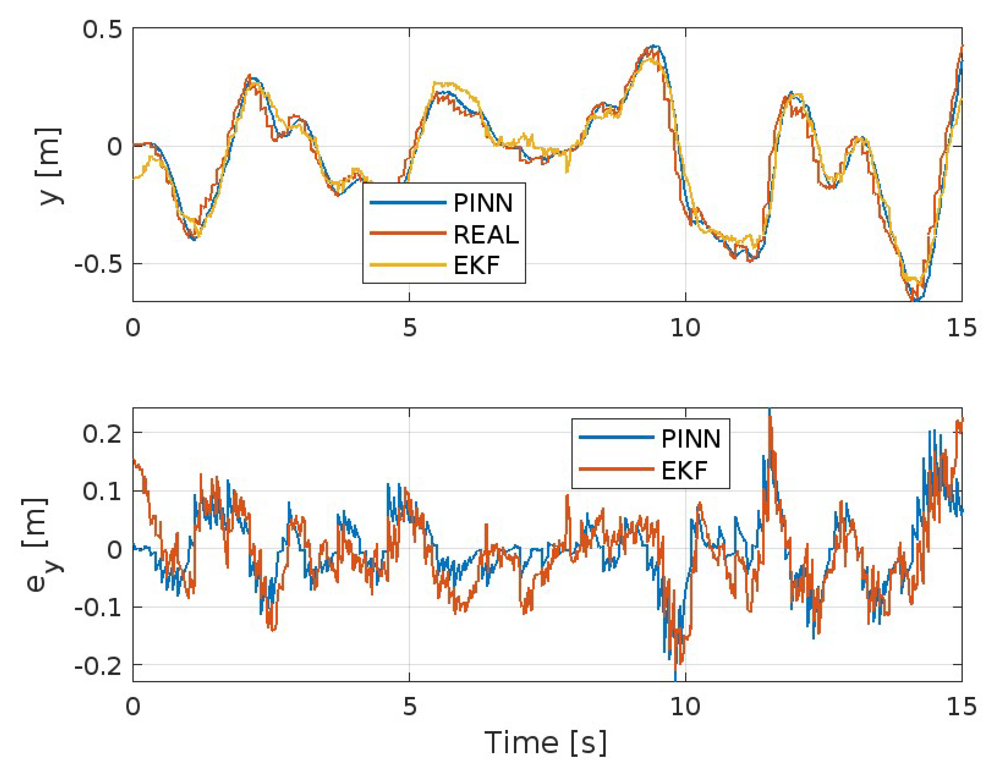
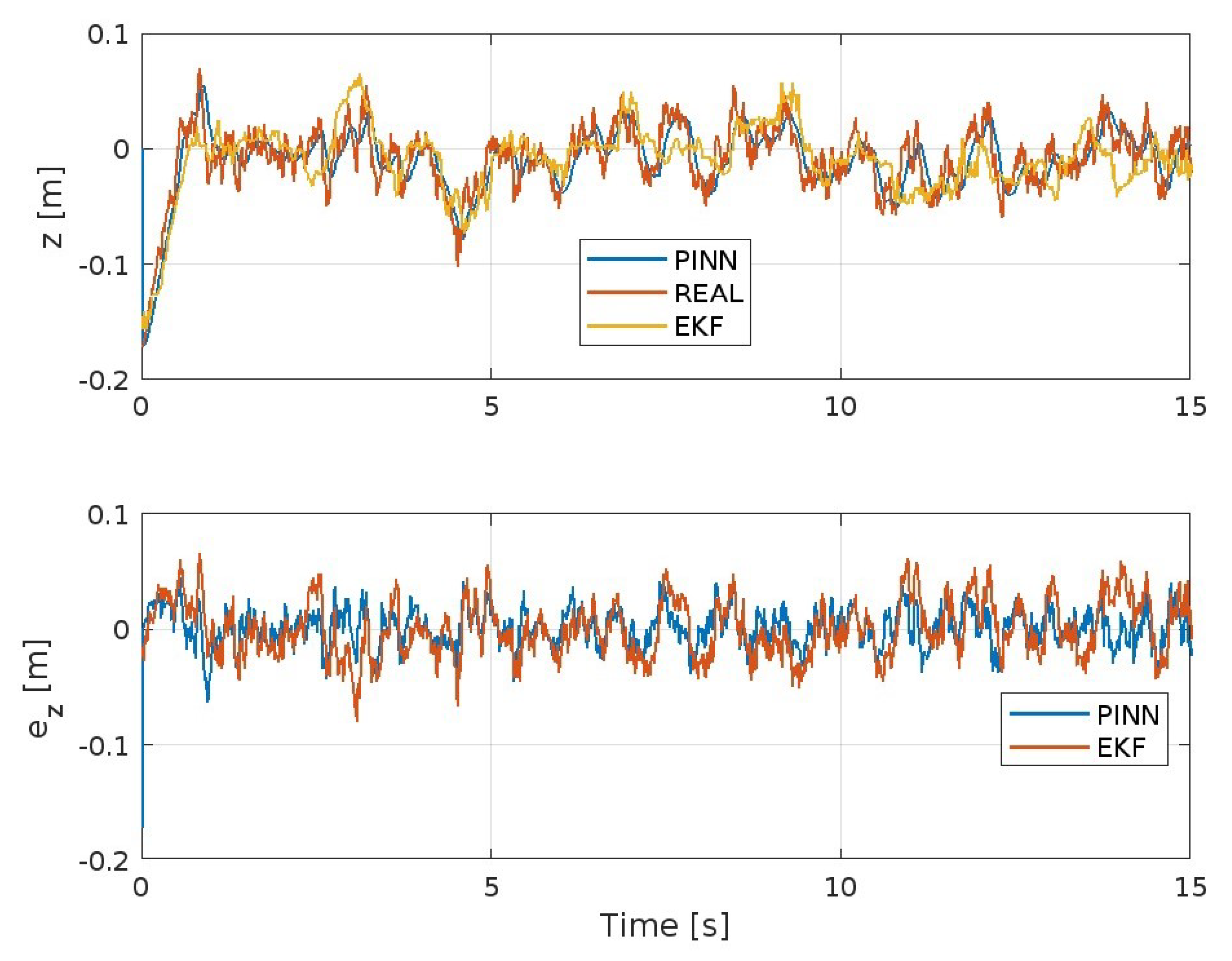
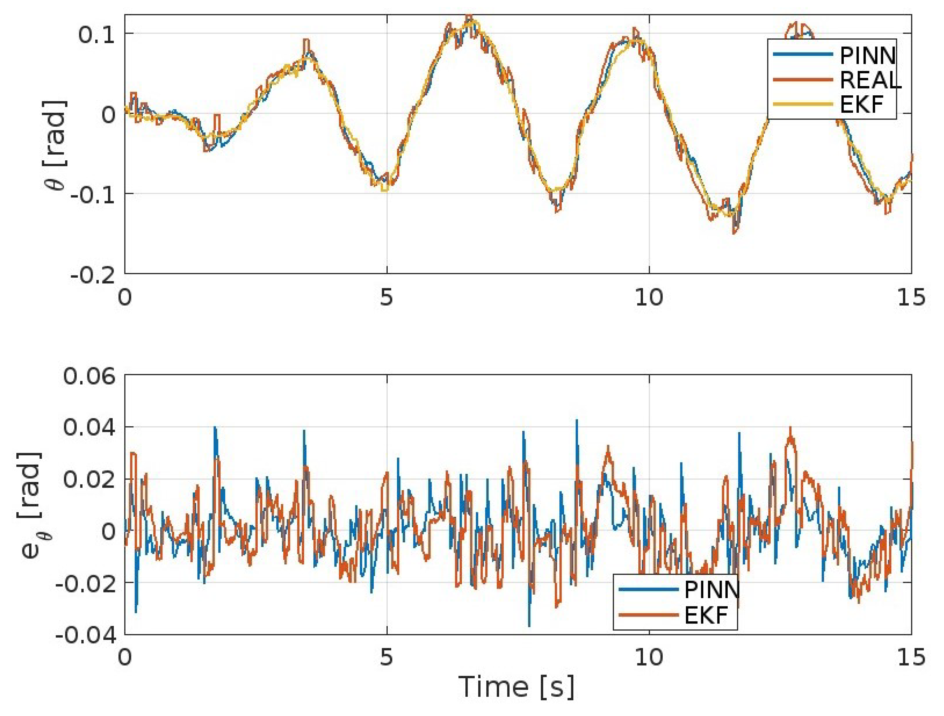
4.2. Model and Performance Comparison

To assess the effectiveness of the proposed Physics-Informed Neural Networks method and to make a comparison with the Extended Kalman Filter-based model identification approach outlined in Section 3, a simulation of the quadrotor system described in Section 2 was conducted using Simulink from MATLAB^® (https://ww2.mathworks.cn/en/?s_tid=gn_logo (accessed on 25 November 2024)). We want to underline that we have available measured data in limited quantities that link the input and output (corresponding to the state). This makes the problem difficult, and a hybrid approach between the use of neural networks and impositions of physical laws represents an excellent compromise between the results obtained and computational load. In

Table 2. Actual parameter values.

Parameter	Value	Units	Known for EKF	Known for PINNs
m	0.65	kg	YES	NO
d	0.165	m	YES	NO
$J_x$	0.03	kg·m2	NO	NO
$J_y$	0.025	kg·m2	NO	NO
$J_z$	0.045	kg·m2	NO	NO
b	3.50	N/rad/s	NO	NO
k	0.06	N·m/rad/s	NO	NO

, the values of the known and unknown model parameters are reported.

An important factor to take into account and that is a strong point of PINNs is that for them every system parameter is assumed to be unknown, while for the EKF it is assumed that some trivial parameters, such as the mass and the distance of the motors from the center of mass, are known. Furthermore, at the simulation level, noise is added to all measured available data in order to make the simulation more realistic. The considered network is comprised of four layers, with each hidden layer featuring 80 neurons activated by the hyperbolic tangent function.

To evaluate the performance of two proposed system estimators in some missions, various metrics, including Mean Absolute Error (MAE), Mean Square Error (MSE), Integral Squared Error (ISE), Integral Absolute Error (IAE), and Integral Time-weighted Absolute Error (ITAE), have been utilized as comparative indicators for system identification. The performance indices are defined for the output state variables $\widehat{y}$ (the same reasoning applies to other variables) concerning the reference $y_{ref}$ that needs to be tracked across N sampling instances. They are defined as follows:

$$MAE={\displaystyle \frac{{\sum }_{i=1}^N[y_{ref,i}-y_i]}{N}},MSE={\displaystyle \frac{1}{N}}\sum _{i=1}^N{(y_{ref,i}-y_i)}^2$$

$$ISE=\int {(y_{ref}-y)}^{2}dt,IAE=\int \mid y_{ref}-y\mid dt$$

$$ITAE=\int (t\mid y_{ref}-y\mid )dt$$

where $y_{ref,i}$ and $y_i$, respectively, are the values of the variables $y_{ref}$ and y at sampling time i, and ISE, IAE, and ITAE integrate over time. Furthermore, the gains in the EKF and the architecture, some parameters of the neural network, as well as a weight on the two cost functionals considered to calculate MSE in the PINNs assume an important value for evaluating the results. Some preliminary findings are reported in

Table 3. Performance indices for the x model errors expressed in meters.

	MAE	MSE	ISE	IAE	ITAE
EKF	0.0514	0.0039	5.8711	77.17	599.94
PINNs	0.0367	0.0022	3.3427	55.07	432.52

,

Table 4. Performance indices for the y model errors expressed in meters.

	MAE	MSE	ISE	IAE	ITAE
EKF	0.0533	0.0047	7.0927	79.96	638.23
PINNs	0.0426	0.0033	4.8822	64	543.46

,

Table 5. Performance indices for the z model errors expressed in meters.

	MAE	MSE	ISE	IAE	ITAE
EKF	0.0198	5.85 $\times {10}^{-4}$	0.8786	29.71	229.05
PINNs	0.0135	2.99 $\times {10}^{-4}$	0.4491	20.3	147.99

,

Table 6. Performance indices for the $\varphi$ model errors expressed in radians.

	MAE	MSE	ISE	IAE	ITAE
EKF	0.0133	4.4527 $\times {10}^{-4}$	0.4204	20.02	163.38
PINNs	0.0103	2.801 $\times {10}^{-4}$	0.2656	15.44	128.97

,

Table 7. Performance indices for the $\theta$ model errors expressed in radians.

	MAE	MSE	ISE	IAE	ITAE
EKF	0.0107	1.81 $\times {10}^{-4}$	0.2718	16.11	130.64
PINNs	0.0085	1.27 $\times {10}^{-4}$	0.1838	12.78	102.45

and

Table 8. Performance indices for the $\psi$ model errors expressed in radians.

	MAE	MSE	ISE	IAE	ITAE
EKF	0.0234	8.92 $\times {10}^{-4}$	0.7541	35.07	269.87
PINNs	0.0149	5.53 $\times {10}^{-4}$	0.5828	22.39	170.66

, illustrating the disparity between the EKF and PINNs estimators in each performance metric of the monitored variables for the x position (Table 3), y position (Table 4), z position (Table 5), $\varphi$ roll angle (Table 6), $\theta$ pitch angle (Table 7), and $\psi$ yaw angle (Table 8).

Figure 3, Figure 4, Figure 5, Figure 6, Figure 7 and Figure 8 show the trends of the Extended Kalman Filter and PINNs to approximate the real system, respectively, for position x, y, z, and the angles $\varphi$, $\theta$, and $\psi$. Both methods will achieve excellent results considering the type of maneuver presented here and the disturbances present. But it is evident that the PINNs outperform the EKF, with the additional strength of requiring a reduced computational effort, despite the fact they require training prior to their use or during the simulation.

5. Conclusions

In this study, we explored the feasibility of using a physics-informed machine learning method, specifically Physics-Informed Neural Networks, to identify nonlinear system models for quadrotors, especially when real-world input–output data are limited. We investigated the potential of PINNs to replace complex nonlinear dynamics with simpler, computationally efficient approximations. By utilizing automatic differentiation, PINNs allow for the straightforward and cost-effective calculation of state derivatives. We compared the performance of PINNs with the Extended Kalman Filter, a well-established method known for its superior performance. Our simulations, conducted on both spatial and orientation variables, demonstrated excellent results from both techniques. However, PINNs outperformed the EKF in terms of error levels compared to real data and computational efficiency. While PINNs require a significant initial training effort, they offer a more efficient and accurate solution once trained.

We plan to extend this research by conducting a comparative computational analysis and exploring the impact of varying identification parameters like $\gamma$. This will help us understand the performance of the hybrid weighted data-driven model-based approach. A subsequent research endeavor could entail the utilization of this system-estimation approach in conjunction with model-based controllers, followed by experimental validation on drone systems. Such an approach would facilitate a thorough assessment of both precision performance and energy consumption metrics with a larger number of available data.

References

1. Wang, J.; Ricardo, A.R.M.; Jorge, J.L.S. Introducing system identification strategy into Model Predictive Control. J. Syst. Sci. Complex. 2020, 33, 1402–1421. [Google Scholar] [CrossRef]
2. Forssell, U.; Lindskog, P. Combining Semi-Physical and Neural Network modeling: An example of its usefulness. IFAC Proc. Vol. 1997, 30, 767–770. [Google Scholar] [CrossRef]
3. Fu, L.; Li, P. The Research Survey of System Identification Method. In Proceedings of the 5th International Conference on Intelligent Human-Machine Systems and Cybernetics, Hangzhou, China, 26–27 August 2013; pp. 397–401. [Google Scholar] [CrossRef]
4. Gueho, D.; Singla, P.; Majji, M.; Juang, J.-N. Advances in System Identification: Theory and Applications. In Proceedings of the 60th IEEE Conference on Decision and Control, Austin, TX, USA, 14–17 December 2021; pp. 22–30. [Google Scholar] [CrossRef]
5. Ho, B.L.; Kalman, R.E. Editorial: Effective construction of linear state-variable models from input/output functions: Die Konstruktion von linearen Modeilen in der Darstellung durch Zustandsvariable aus den Beziehungen für Ein-und Ausgangsgrößen. Automatisierungstechnik 1966, 14, 545–548. [Google Scholar] [CrossRef]
6. Kalman, R.E. Mathematical Description of Linear Dynamical Systems. J. Soc. Ind. Appl. Math. Ser. A Control. 1963, 1, 152–192. [Google Scholar] [CrossRef]
7. Chen, C.W.; Lee, G.; Juang, J.-N. Several recursive techniques for observer/Kalman filter system identification from data. In Proceedings of the Guidance, Navigation and Control Conference, Hilton Head Island, SC, USA, 10–12 August 1992. [Google Scholar] [CrossRef]
8. Germani, A.; Manes, C.; Palumbo, P. Polynomial extended Kalman filter. IEEE Trans. Autom. Control. 2005, 50, 2059–2064. [Google Scholar] [CrossRef]
9. Peyada, N.K.; Sen, A.; Ghosh, A.K. Aerodynamic characterization of HANSA-3 aircraft using equation error, maximum likelihood and filter error methods. In Proceedings of the International MultiConference of Engineers and Computer Scientists, Hong Kong, 19–21 March 2008. [Google Scholar] [CrossRef]
10. Bianchi, D.; Borri, A.; Di Benedetto, M.D.; Di Gennaro, S. Active Attitude Control of Ground Vehicles with Partially Unknown Model. IFAC-PapersOnLine 2020, 53, 14420–14425. [Google Scholar] [CrossRef]
11. Rodrigues, L.; Givigi, S. System Identification and Control Using Quadratic Neural Networks. IEEE Control. Syst. Lett. 2023, 7, 2209–2214. [Google Scholar] [CrossRef]
12. Cavone, G.; Epicoco, N.; Carli, R.; Del Zotti, A.; Ribeiro Pereira, J.P.; Dotoli, M. Parcel delivery with drones: Multi-criteria analysis of trendy system architectures. In Proceedings of the 29th Mediterranean Conference on Control and Automation, Puglia, Italy, 22–25 June 2021; pp. 693–698. [Google Scholar] [CrossRef]
13. Carli, R.; Cavone, G.; Epicoco, N.; Di Ferdinando, M.; Scarabaggio, P.; Dotoli, M. Consensus-Based Algorithms for Controlling Swarms of Unmanned Aerial Vehicles; Lecture Notes in Computer Science; Springer: Cham, Switzerland, 2020; Volume 12338, pp. 84–99. [Google Scholar] [CrossRef]
14. Bianchi, D.; Borri, A.; Di Gennaro, S.; Preziuso, M. UAV trajectory control with rule-based minimum-energy reference generation. In Proceedings of the European Control Conference, London, UK, 12–15 July 2022; pp. 1497–1502. [Google Scholar] [CrossRef]
15. Stiasny, J.; Misyris, G.S.; Chatzivasileiadis, S. Physics-Informed Neural Networks for Non-linear System Identification for Power System Dynamics. In Proceedings of the 2021 IEEE Madrid PowerTech, Madrid, Spain, 28 June–2 July 2021. [Google Scholar] [CrossRef]
16. Liu, X.; Cheng, W.; Xing, J.; Chen, X.; Zhao, Z.; Zhang, R.; Huang, Q.; Lu, J.; Zhou, H.; Zheng, W.X.; et al. Physics-Informed Neural Network for system identification of rotors. IFAC-PapersOnLine 2024, 58, 307–312. [Google Scholar] [CrossRef]
17. Liu, T.; Meidani, H. Physics-Informed Neural Networks for System Identification of Structural Systems with a Multiphysics Damping Model. J. Eng. Mech. 2023, 149, 04023079. [Google Scholar] [CrossRef]
18. Li, H.W.X.; Lu, L.; Cao, Q. Motion estimation and system identification of a moored buoy via Physics-Informed Neural Network. Appl. Ocean. Res. 2023, 138, 103677. [Google Scholar] [CrossRef]
19. Malinzi, J.; Gwebu, S.; Motsa, S. Determining COVID-19 Dynamics Using Physics Informed Neural Networks. Axioms 2022, 11, 121. [Google Scholar] [CrossRef]
20. D’Ambrosio, A.; Furfaro, R. Learning Fuel-Optimal Trajectories for Space Applications via Pontryagin Neural Networks. Aerospace 2024, 11, 228. [Google Scholar] [CrossRef]
21. Singh, V.; Harursampath, D.; Dhawan, S.; Sahni, M.; Saxena, S.; Mallick, R. Physics-Informed Neural Network for Solving a One-Dimensional Solid Mechanics Problem. Modelling 2024, 5, 1532–1549. [Google Scholar] [CrossRef]
22. Li, Y.; Liu, L. Physics-Informed Neural Network-Based Nonlinear Model Predictive Control for Automated Guided Vehicle Trajectory Tracking. World Electr. Veh. J. 2024, 15, 460. [Google Scholar] [CrossRef]
23. Trahan, C.; Loveland, M.; Dent, S. Quantum Physics-Informed Neural Networks. Entropy 2024, 26, 649. [Google Scholar] [CrossRef] [PubMed]
24. Güven, K.; Şamiloğlu, A.T. System Identification of an Aerial Delivery System with a Ram-Air Parachute Using a NARX Network. Aerospace 2022, 9, 443. [Google Scholar] [CrossRef]
25. Zheng, X.; Liu, S.; Yu, Z.; Luo, C. A New Method for Dynamical System Identification by Optimizing the Control Parameters of Legendre Multiwavelet Neural Network. Mathematics 2023, 11, 4913. [Google Scholar] [CrossRef]
26. Peña-García, R.; Velázquez-Sánchez, R.D.; Gómez-Daza-Argumedo, C.; Escobedo-Alva, J.O.; Tapia-Herrera, R.; Meda-Campaña, J.A. Physics-Based Aircraft Dynamics Identification Using Genetic Algorithms. Aerospace 2024, 11, 142. [Google Scholar] [CrossRef]
27. Gu, W.; Primatesta, S.; Rizzo, A. Physics-Informed Neural Network for Quadrotor Dynamical Modeling. Robot. Auton. Syst. 2024, 171, 104569. [Google Scholar] [CrossRef]
28. Bianchi, D.; Borri, A.; Cappuzzo, F.; Di Gennaro, S. Quadrotor Trajectory Control Based on Energy-Optimal Reference Generator. Drones 2024, 8, 29. [Google Scholar] [CrossRef]
29. Bianchi, D.; Di Gennaro, S.; Di Ferdinando, M.; Lua, C.A. Robust Control of UAV with Disturbances and Uncertainty Estimation. Machines 2023, 11, 352. [Google Scholar] [CrossRef]
30. Hughes, P.C. Spacecraft Attitude Dynamics; Dover Publications, Inc.: Mineola, NY, USA, 1986. [Google Scholar]
31. Nagaty, A.; Saeedi, S.; Thibault, C.; Seto, M.; Li, H. Control and Navigation Framework for Quadrotor Helicopters. J. Intell. Robot. Syst. 2013, 70, 1–12. [Google Scholar] [CrossRef]
32. Fujii, K. Extended Kalman Filter; Refernce Manual; The ACFA-Sim-J Group: Tokyo, Japan, 2013. [Google Scholar]
33. Raissi, M.; Perdikaris, P.; Karniadakis, G.E. Physics-Informed Neural Networks: A deep learning framework for solving forward and inverse problems involving nonlinear partial differential equations. J. Comput. Phys. 2019, 378, 686–707. [Google Scholar] [CrossRef]
34. Kumar, P.; Batra, S.; Raman, B. Deep neural network hyper-parameter tuning through twofold genetic approach. Soft Comput. 2021, 25, 8747–8771. [Google Scholar] [CrossRef]
Figure 1. Quadrotor orientation using Euler angles.
Drones 08 00716 g001
Figure 2. PINNs architecture. It functions by employing its own output prediction as the initial state.
Drones 08 00716 g002
Figure 3. Position x-axis and corresponding error.
Drones 08 00716 g003
Figure 4. Position y-axis and corresponding error.
Drones 08 00716 g004
Figure 5. Position z-axis and corresponding error.
Drones 08 00716 g005
Figure 6. Roll angle ϕ and corresponding error.
Drones 08 00716 g006
Figure 7. Pitch angle θ and corresponding error.
Drones 08 00716 g007
Figure 8. Yaw angle ψ and corresponding error.
Drones 08 00716 g008