
Wind Pressure Orthogonal Decomposition Anemometer: A Wind Measurement Device for Multi-Rotor UAVs

 ,
,
Abstract
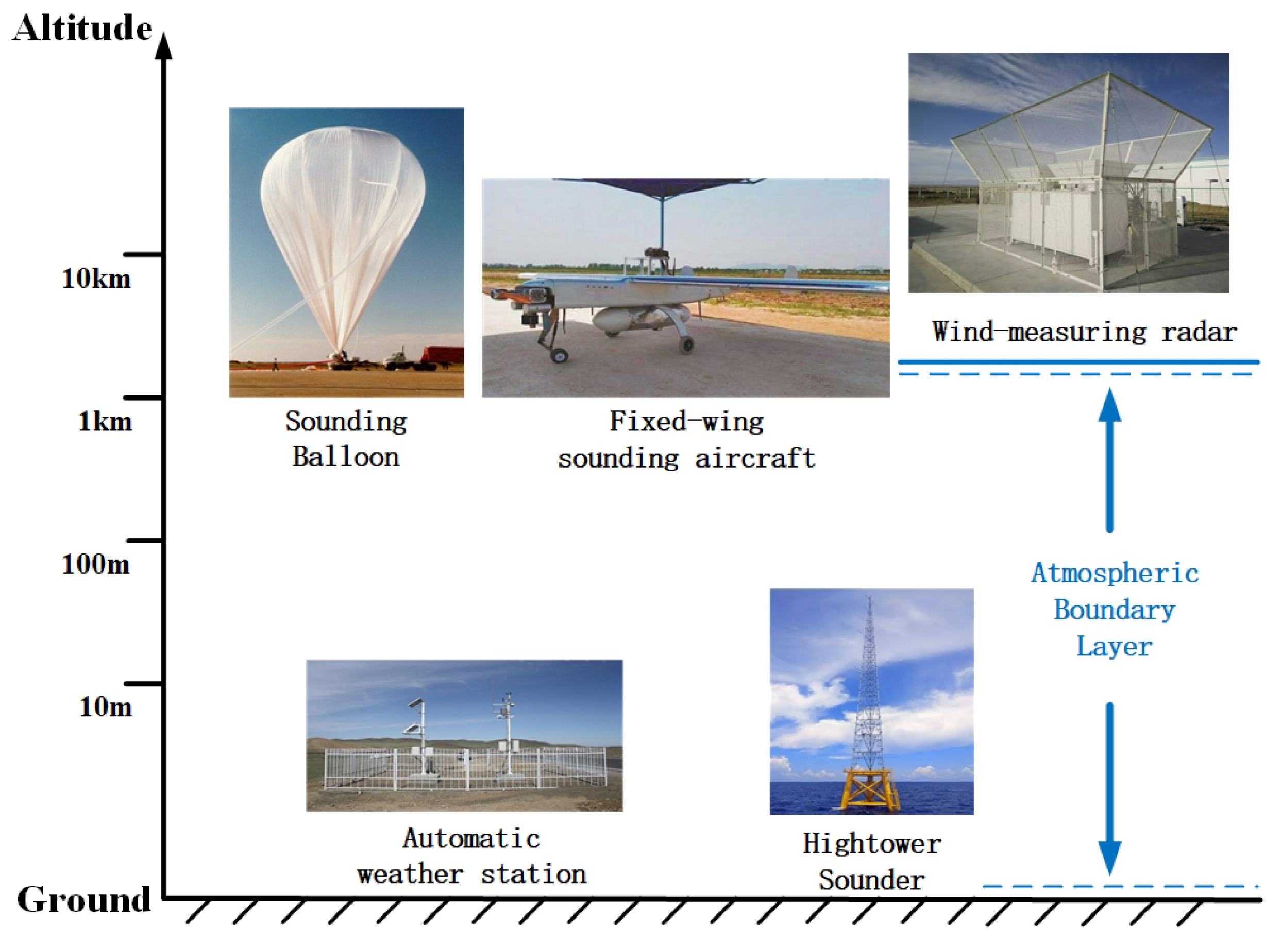
1. Introduction
2. Flow Field Analysis of Quadrotor UAV
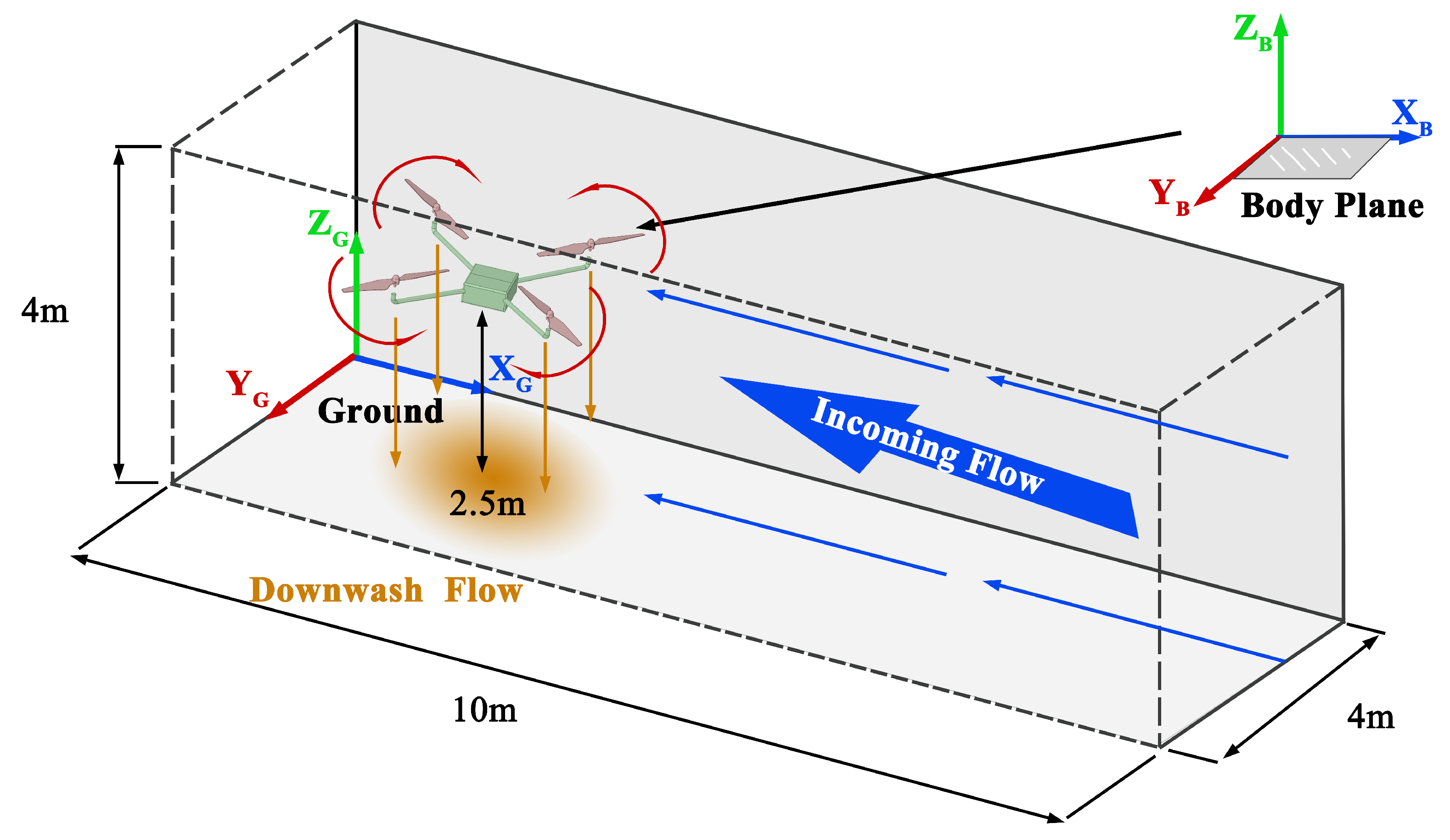
2.1. Experimental Setup for Wind Field Analysis
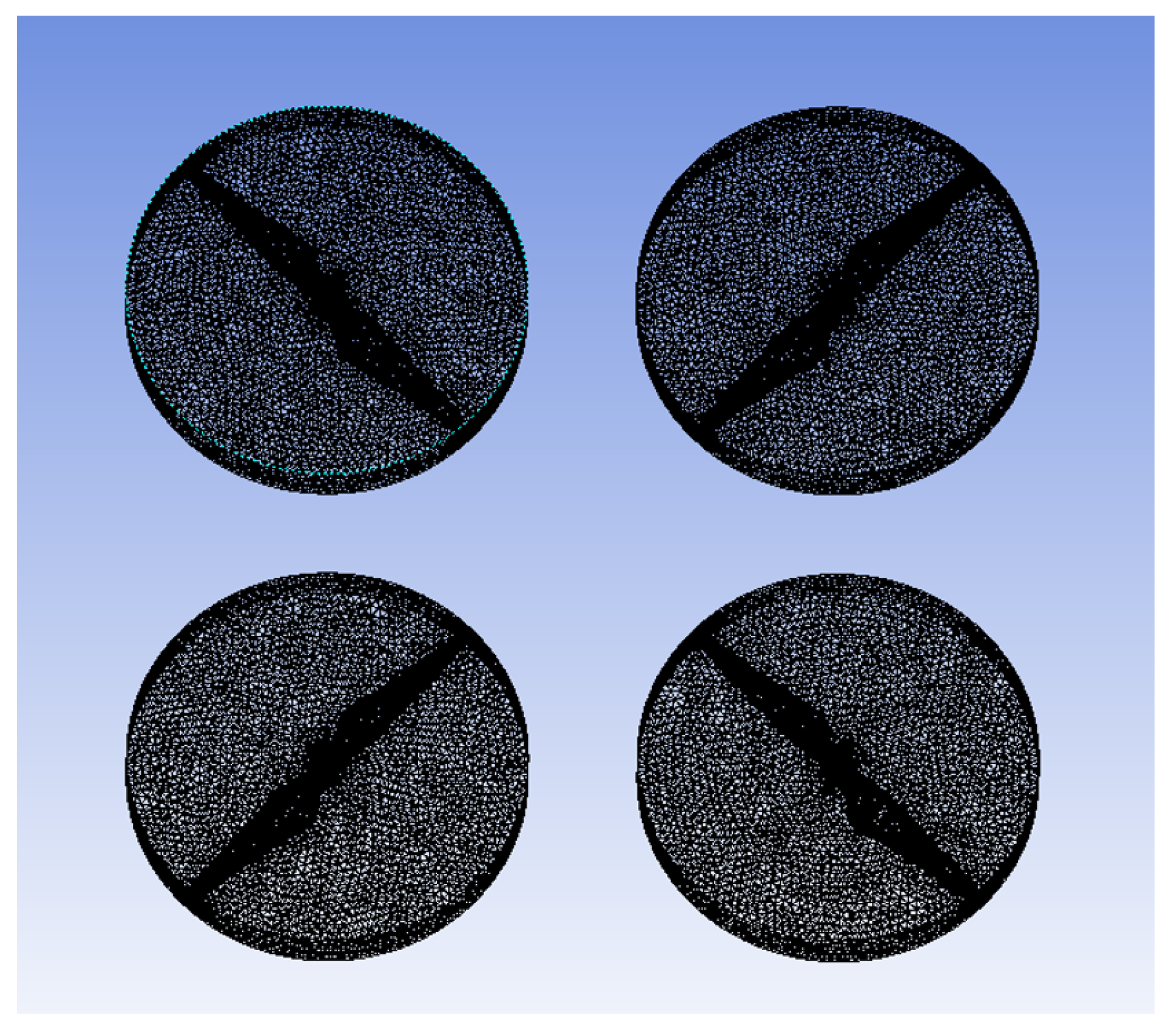
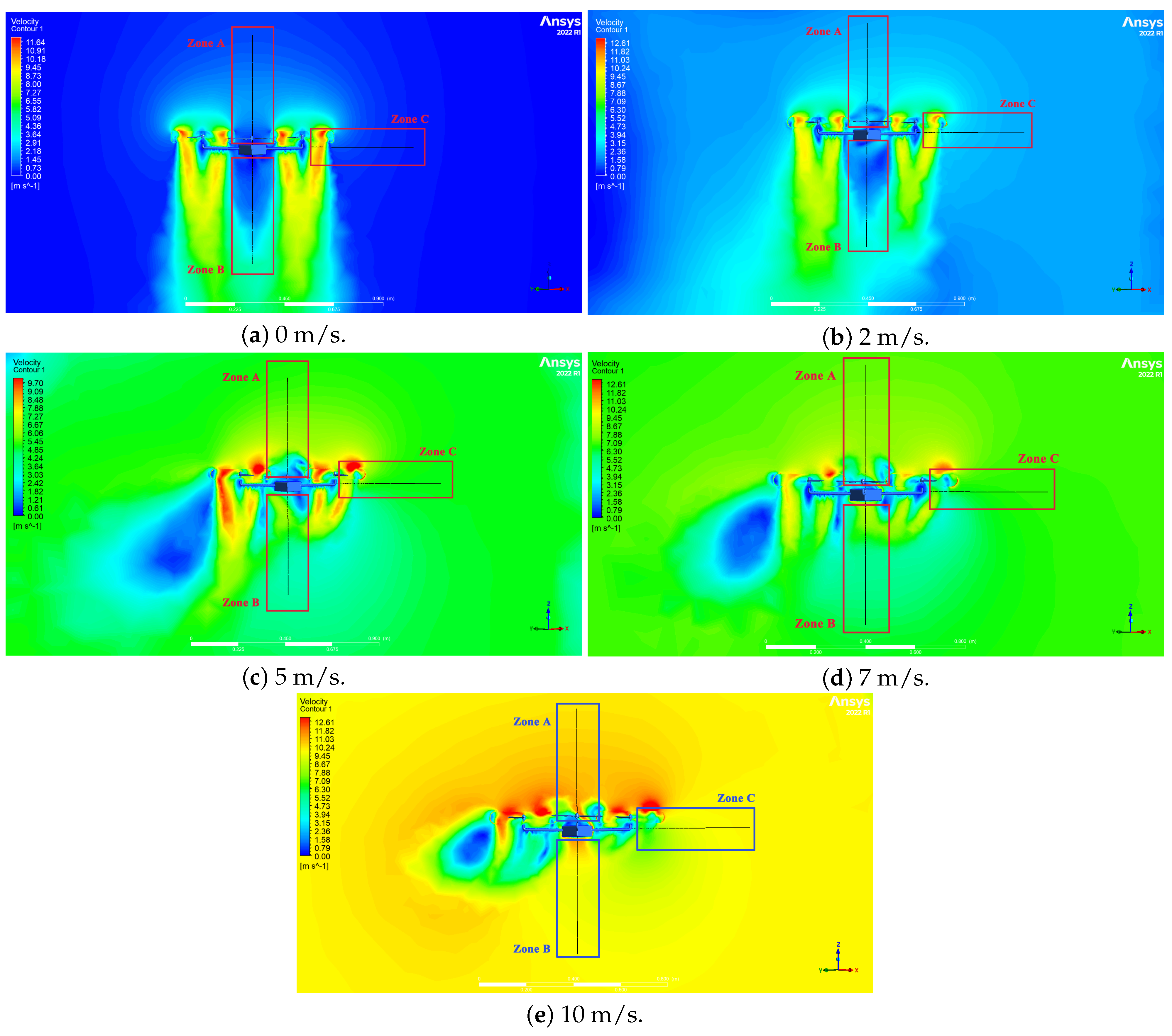
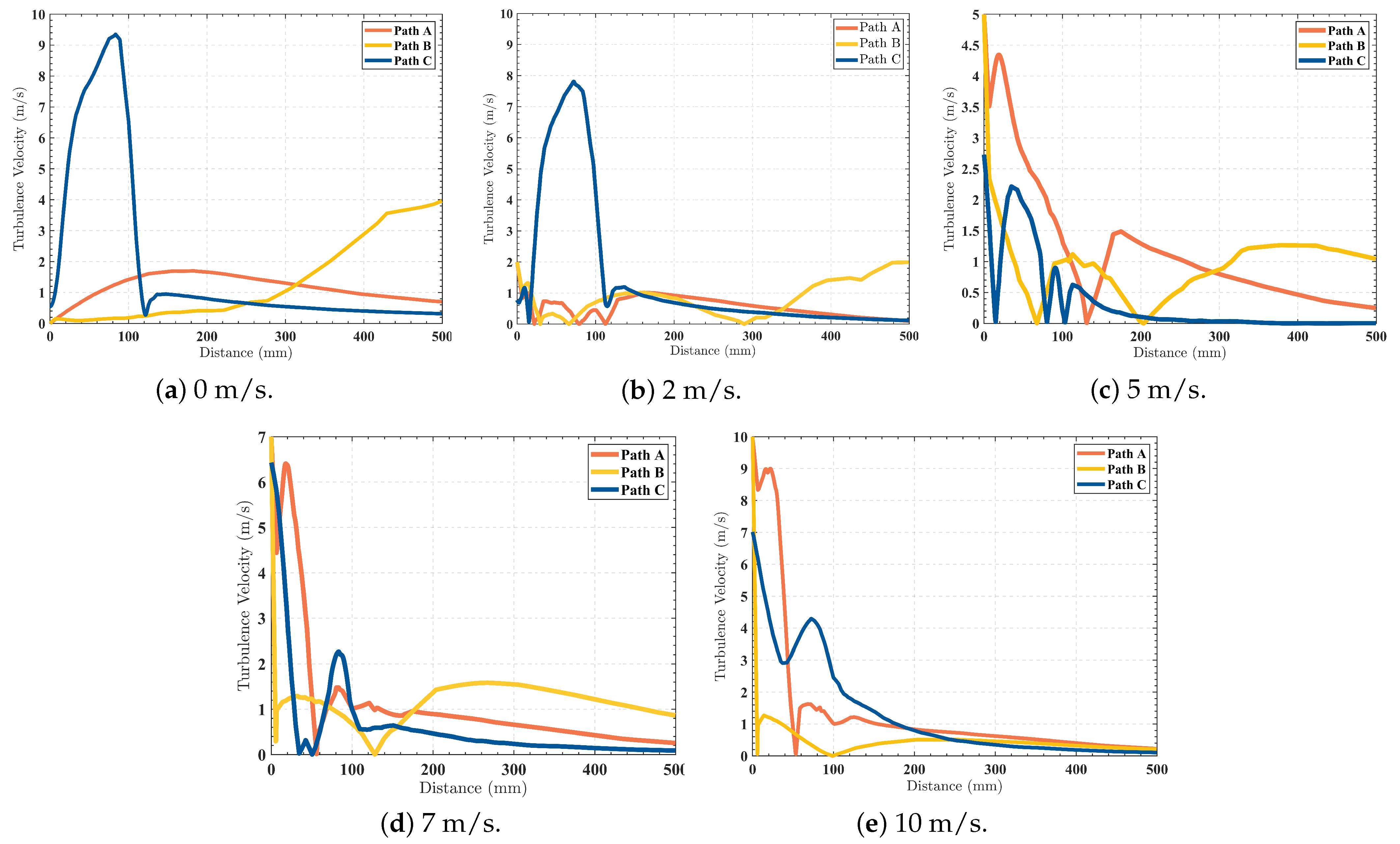
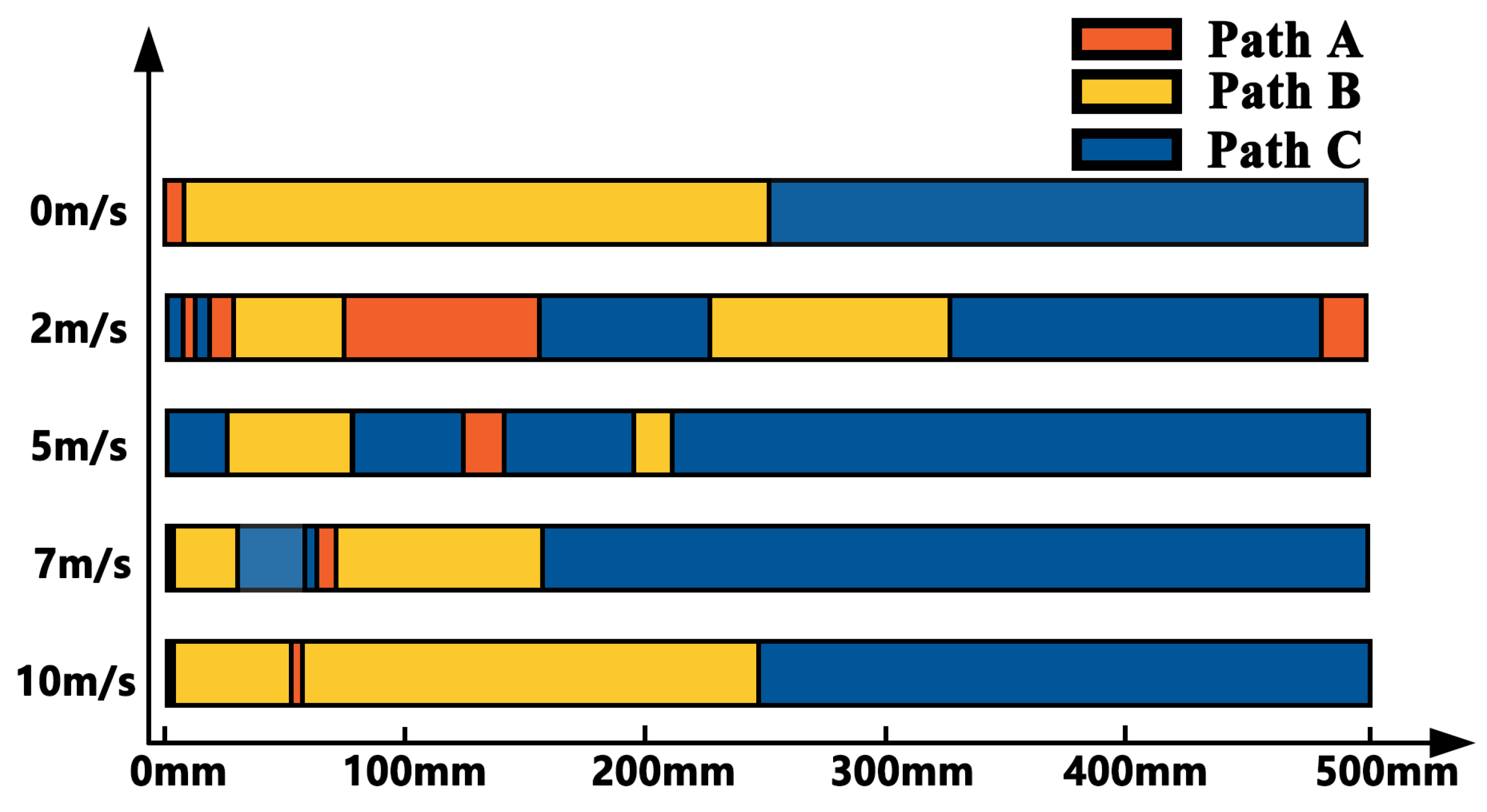
2.2. Flow Field Analysis of the Quadrotor UAV Flight
3. The Wind Pressure Orthogonal Decomposition Wind Measurement Method
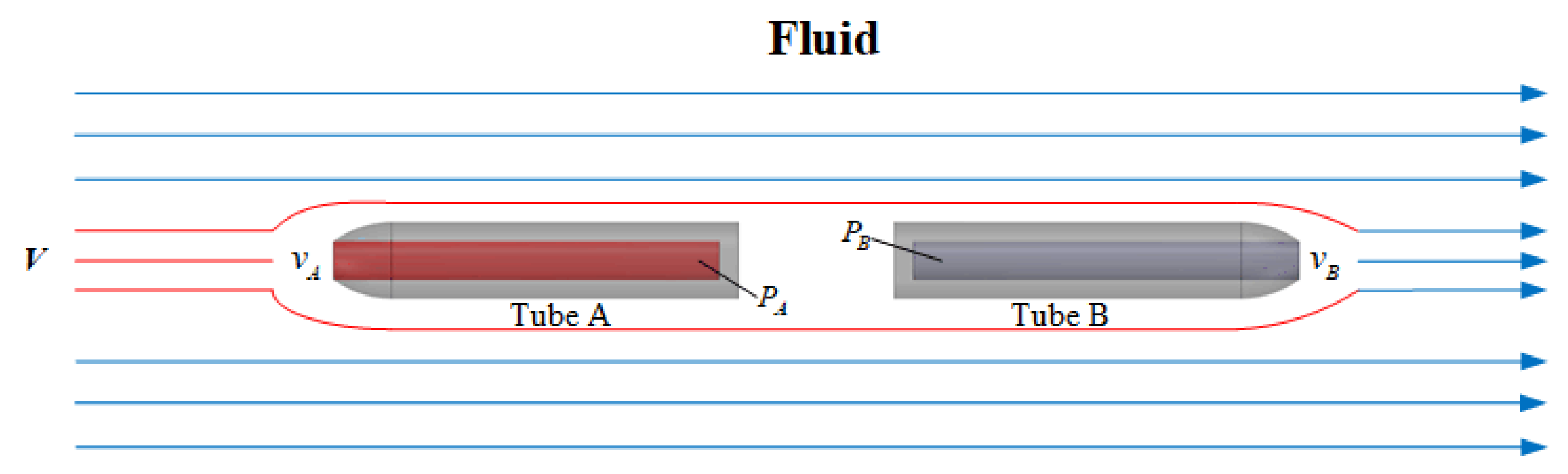
3.1. Wind Measurement Principles
3.2. Attitude—Wind Velocity Correction Algorithm
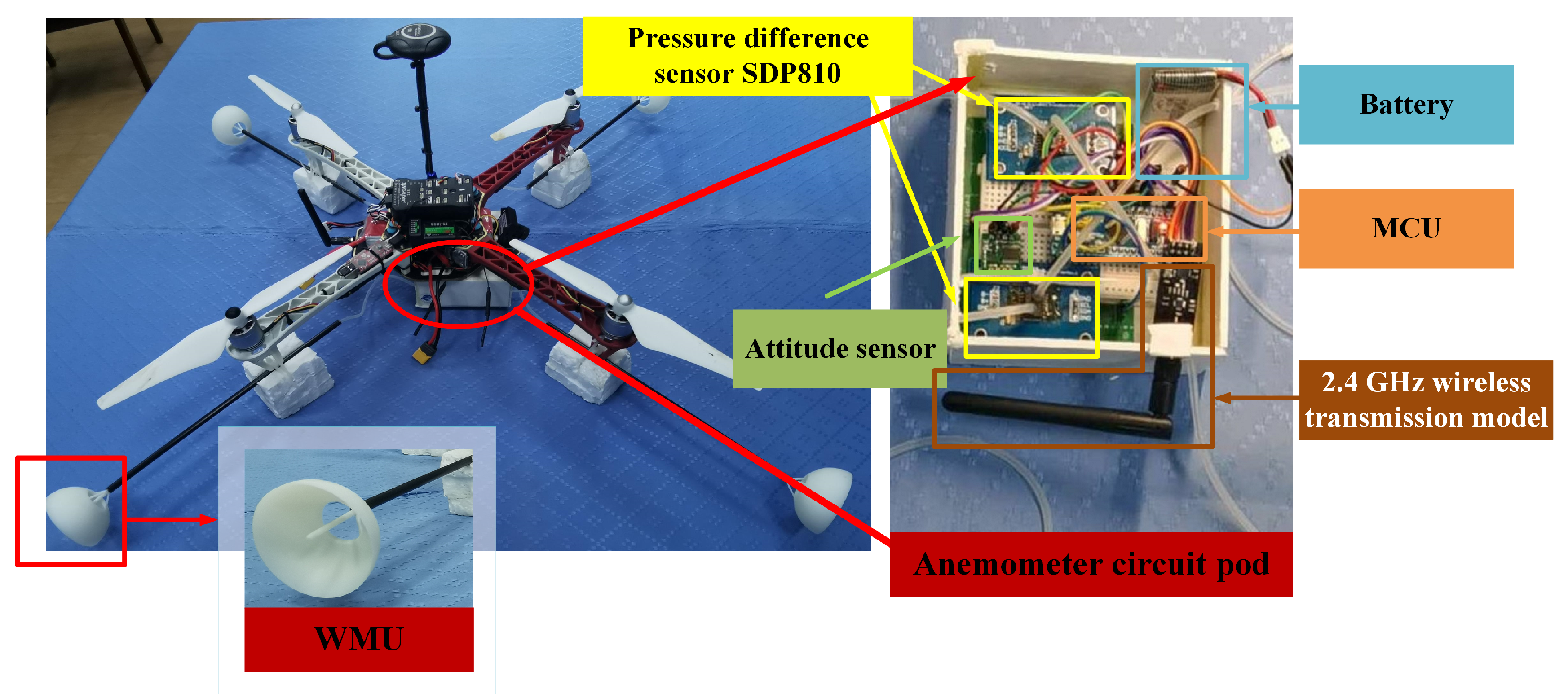
4. WPOD Anemometer
4.1. WPOD Anemometer Construction
4.2. WMU Performance Verification and Calibration
5. Field Experiment and Analysis
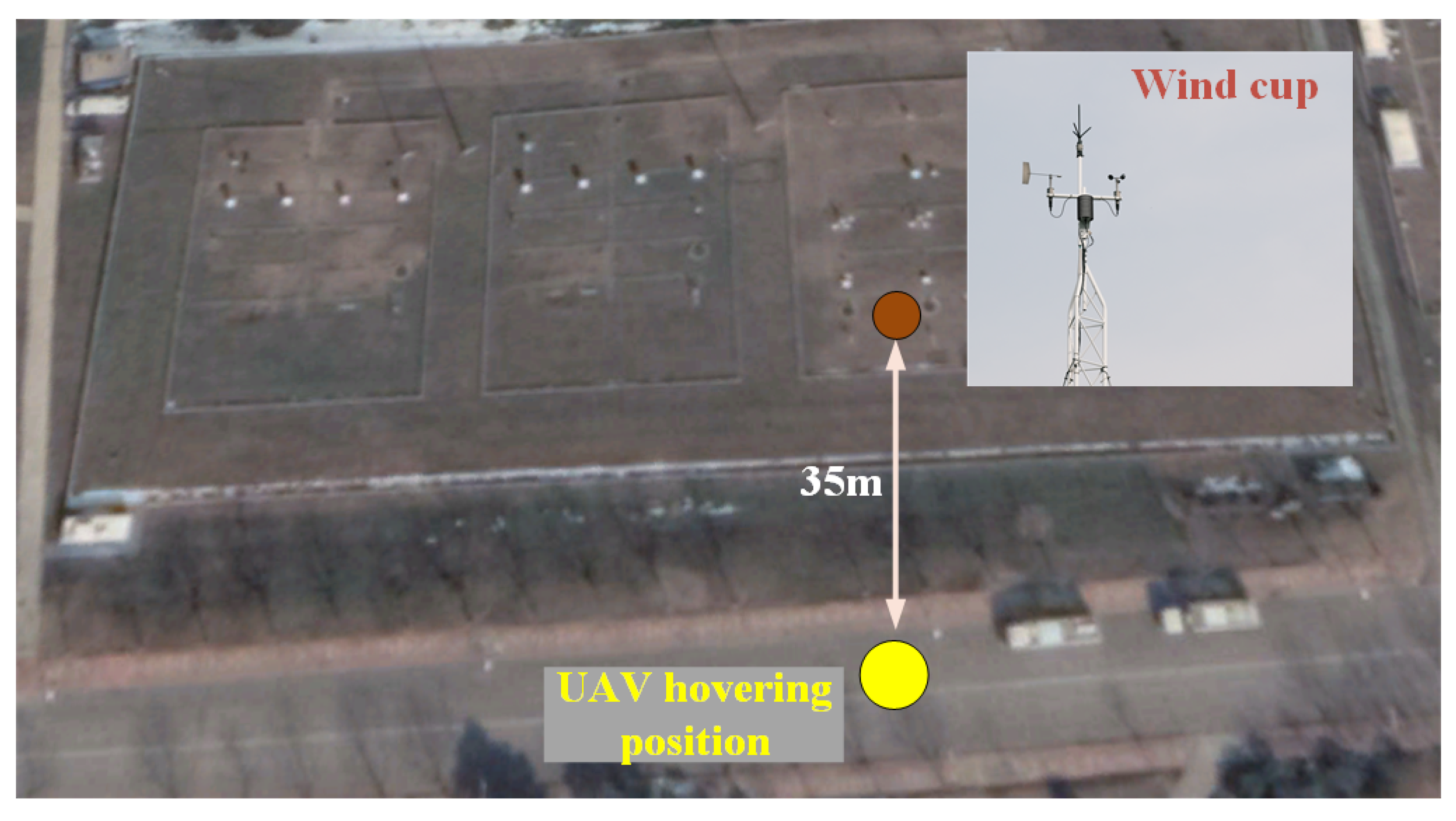
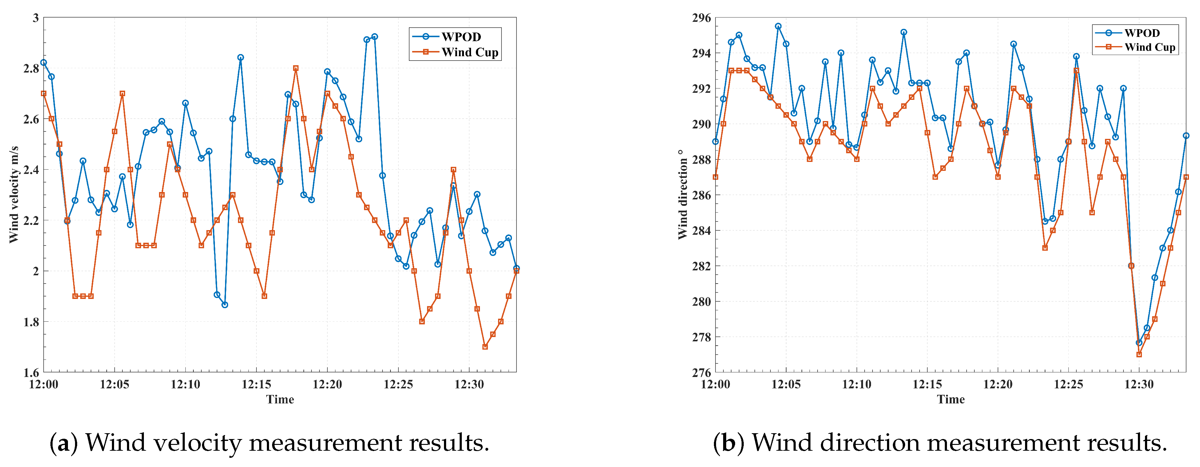
5.1. Hovering Wind Measurement Experiment
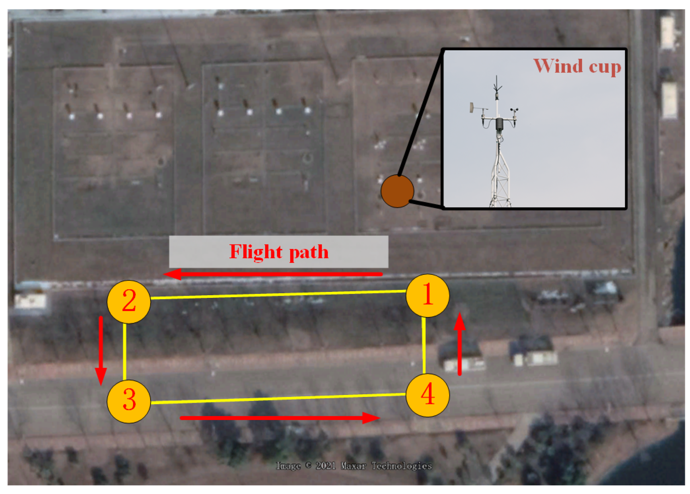
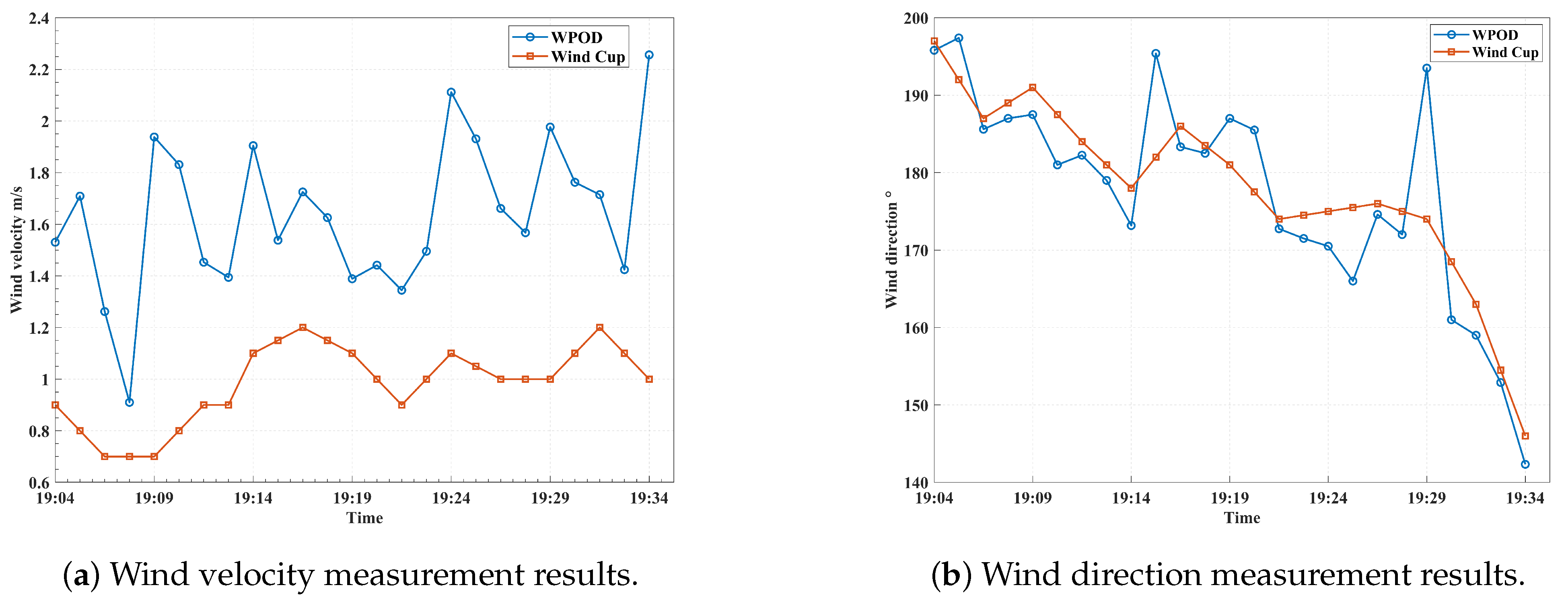
5.2. Moving Wind Measurement Experiment
6. Discussion
7. Conclusions
Author Contributions
Funding
Data Availability Statement
Acknowledgments
Conflicts of Interest
References
- Jozef, G.; Cassano, J.; Dahlke, S.; de Boer, G. Testing the efficacy of atmospheric boundary layer height detection algorithms using uncrewed aircraft system data from MOSAiC. Atmos. Meas. Tech. 2022, 15, 4001–4022. [Google Scholar] [CrossRef]
- Vincent, V.; Chiu, E.; Tae, K.S.; Bukhori, I.; Setiyadi, S. Automatic Wireless Mobile Weather Station. J. Electr. Electron. Eng. 2020, 2, 54–59. [Google Scholar] [CrossRef]
- Rodríguez, O.; Bech, J.; Soriano, J.d.D.; Gutiérrez, D.; Castán, S. A methodology to conduct wind damage field surveys for high-impact weather events of convective origin. Nat. Hazards Earth Syst. Sci. 2020, 20, 1513–1531. [Google Scholar] [CrossRef]
- Kim, J.h.; woo Lee, D.; Cho, K.r.; Jo, S.y.; Kim, J.h.; Min, C.o.; Han, D.i.; Cho, S.j. Development of an electro-optical system for small UAV. Aerosp. Sci. Technol. 2010, 14, 505–511. [Google Scholar] [CrossRef]
- Rautenberg, A.; Graf, M.S.; Wildmann, N.; Platis, A.; Bange, J. Reviewing wind measurement approaches for fixed-wing unmanned aircraft. Atmosphere 2018, 9, 422. [Google Scholar] [CrossRef]
- Lehner, M.; Whiteman, C.D.; Hoch, S.W.; Jensen, D.; Pardyjak, E.R.; Leo, L.S.; Di Sabatino, S.; Fernando, H.J. A case study of the nocturnal boundary layer evolution on a slope at the foot of a desert mountain. J. Appl. Meteorol. Climatol. 2015, 54, 732–751. [Google Scholar] [CrossRef]
- Kalverla, P.C.; Duine, G.J.; Steeneveld, G.J.; Hedde, T. Evaluation of the Weather Research and Forecasting Model in the Durance Valley complex terrain during the KASCADE field campaign. J. Appl. Meteorol. Climatol. 2016, 55, 861–882. [Google Scholar] [CrossRef]
- Ma, S.; Wang, G.; Pan, Y.; Wang, L. An analytical method for wind measurements by a mini-aircraft. Chin. J. Atmos. Sci. 1999, 23, 377–384. [Google Scholar]
- Zhang, Y.; Dong, T.; Liu, Y. Design of meteorological element detection platform for atmospheric boundary layer based on UAV. Int. J. Aerosp. Eng. 2017, 2017, 1831676. [Google Scholar] [CrossRef]
- Johansen, T.A.; Cristofaro, A.; Sørensen, K.; Hansen, J.M.; Fossen, T.I. On estimation of wind velocity, angle-of-attack and sideslip angle of small UAVs using standard sensors. In Proceedings of the 2015 International Conference on Unmanned Aircraft Systems (ICUAS), Denver, CO, USA, 9–12 June 2015; pp. 510–519. [Google Scholar]
- Witte, B.M.; Singler, R.F.; Bailey, S.C. Development of an unmanned aerial vehicle for the measurement of turbulence in the atmospheric boundary layer. Atmosphere 2017, 8, 195. [Google Scholar] [CrossRef]
- Wenz, A.; Johansen, T.A. Estimation of wind velocities and aerodynamic coefficients for UAVs using standard autopilot sensors and a moving horizon estimator. In Proceedings of the 2017 International Conference on Unmanned Aircraft Systems (ICUAS), Miami, FL, USA, 13–16 June 2017; pp. 1267–1276. [Google Scholar]
- Axisa, D.; DeFelice, T.P. Modern and prospective technologies for weather modification activities: A look at integrating unmanned aircraft systems. Atmos. Res. 2016, 178, 114–124. [Google Scholar] [CrossRef]
- Lawrence, D.A.; Balsley, B.B. High-resolution atmospheric sensing of multiple atmospheric variables using the DataHawk small airborne measurement system. J. Atmos. Ocean. Technol. 2013, 30, 2352–2366. [Google Scholar] [CrossRef]
- Van den Kroonenberg, A.; Martin, T.; Buschmann, M.; Bange, J.; Vörsmann, P. Measuring the wind vector using the autonomous mini aerial vehicle M2AV. J. Atmos. Ocean. Technol. 2008, 25, 1969–1982. [Google Scholar] [CrossRef]
- Xu, Q.; Wei, L.; Nai, K.; Liu, S.; Rabin, R.M.; Zhao, Q. A radar wind analysis system for nowcast applications. Adv. Meteorol. 2015, 2015, 264515. [Google Scholar] [CrossRef]
- Susko, M. Jimsphere and radar wind profiler turbulence indicators. J. Spacecr. Rocket. 1994, 31, 678–683. [Google Scholar] [CrossRef]
- Zhu, X.; Liu, J.; Bi, D.; Zhou, J.; Diao, W.; Chen, W. Development of all-solid coherent Doppler wind lidar. Chin. Opt. Lett. 2012, 10, 012801. [Google Scholar]
- Bian, Z.; Huang, C.; Chen, D.; Peng, J.; Gao, M.; Dong, Z.; Liu, J.; Cai, H.; Qu, R.; Gong, S. Seed laser frequency stabilization for Doppler wind lidar. Chin. Opt. Lett. 2012, 10, 091405. [Google Scholar] [CrossRef]
- Nuijens, L.; Siebesma, A.P. Boundary layer clouds and convection over subtropical oceans in our current and in a warmer climate. Curr. Clim. Chang. Rep. 2019, 5, 80–94. [Google Scholar] [CrossRef]
- Wetz, T.; Wildmann, N.; Beyrich, F. Distributed wind measurements with multiple quadrotor unmanned aerial vehicles in the atmospheric boundary layer. Atmos. Meas. Tech. 2021, 14, 3795–3814. [Google Scholar] [CrossRef]
- González-Rocha, J.; Woolsey, C.A.; Sultan, C.; De Wekker, S.F. Sensing wind from quadrotor motion. J. Guid. Control Dyn. 2019, 42, 836–852. [Google Scholar] [CrossRef]
- Crowe, D.; Pamula, R.; Cheung, H.Y.; De Wekker, S.F. Two supervised machine learning approaches for wind velocity estimation using multi-rotor copter attitude measurements. Sensors 2020, 20, 5638. [Google Scholar] [CrossRef] [PubMed]
- Allison, S.; Bai, H.; Jayaraman, B. Wind estimation using quadcopter motion: A machine learning approach. Aerosp. Sci. Technol. 2020, 98, 105699. [Google Scholar] [CrossRef]
- Riddell, K.D.A. Design, Testing and Demonstration of a Small Unmanned Aircraft System (SUAS) and Payload for Measuring Wind Speed and Particulate Matter in the Atmospheric Boundary Layer; University of Lethbridge: Lethbridge, AB, Canada, 2014. [Google Scholar]
- Wolf, C.A.; Hardis, R.P.; Woodrum, S.D.; Galan, R.S.; Wichelt, H.S.; Metzger, M.C.; Bezzo, N.; Lewin, G.C.; de Wekker, S.F. Wind data collection techniques on a multi-rotor platform. In Proceedings of the 2017 Systems and Information Engineering Design Symposium (SIEDS), Charlottesville, VA, USA, 28 April 2017; pp. 32–37. [Google Scholar]
- Abichandani, P.; Lobo, D.; Ford, G.; Bucci, D.; Kam, M. Wind measurement and simulation techniques in multi-rotor small unmanned aerial vehicles. IEEE Access 2020, 8, 54910–54927. [Google Scholar] [CrossRef]
- Mallon, C.J.; Muthig, B.J.; Gamagedara, K.; Patil, K.; Friedman, C.; Lee, T.; Snyder, M.R. Measurements of ship air wake using airborne anemometers. In Proceedings of the 55th AIAA Aerospace Sciences Meeting, Grapevine, TX, USA, 9–13 January 2017; p. 0252. [Google Scholar]
- Thorpe, R.L.; McCrink, M.; Gregory, J.W. Measurement of unsteady gusts in an urban wind field using a uav-based anemometer. In Proceedings of the 2018 Applied Aerodynamics Conference, Atlanta, GA, USA, 25–29 June 2018; p. 4218. [Google Scholar]
- Palomaki, R.T.; Rose, N.T.; van den Bossche, M.; Sherman, T.J.; De Wekker, S.F. Wind estimation in the lower atmosphere using multirotor aircraft. J. Atmos. Ocean. Technol. 2017, 34, 1183–1191. [Google Scholar] [CrossRef]
- Li, Z.; Hu, H.; Shen, Y. The influence of rotor rotation of hexacopter on wind measurement accuracy. J. Exp. Fluid Mech. 2019, 33, 7–14. [Google Scholar]
- Li, Z.; Pu, O.; Pan, Y.; Huang, B.; Zhao, Z.; Wu, H. A Study on Measuring the Wind Field in the Air Using a multi-rotor UAV Mounted with an Anemometer. Bound.-Layer Meteorol. 2023, 188, 1–27. [Google Scholar] [CrossRef]
- Donnell, G.W.; Feight, J.A.; Lannan, N.; Jacob, J.D. Wind characterization using onboard IMU of sUAS. In Proceedings of the 2018 Atmospheric Flight Mechanics Conference, Atlanta, GA, USA, 25–29 June 2018; p. 2986. [Google Scholar]
- Hou, T.; Xing, H.; Yang, L. Orthogonal wind pressure vector decomposition wind measurement method based on multi-rotor UAV. Chin. J. Sci. Instrum. 2019, 40, 200–207. [Google Scholar]
- Menter, F. Zonal two equation kw turbulence models for aerodynamic flows. In Proceedings of the 23rd Fluid Dynamics, Plasmadynamics, and Lasers Conference, Orlando, FL, USA, 6–9 July 1993; p. 2906. [Google Scholar]
- Wang, L.; Hou, Q.; Wang, J.; Wang, Z.; Wang, S. Influence of the inner tilt angle on downwash airflow field of multi-rotor UAV based on wireless wind speed acquisition system. Int. J. Agric. Biol. Eng. 2021, 14, 19–26. [Google Scholar] [CrossRef]
- Nguyen, D.T.; Choi, Y.M.; Lee, S.H.; Kang, W. The impact of geometric parameters of a S-type Pitot tube on the flow velocity measurements for greenhouse gas emission monitoring. Flow Meas. Instrum. 2019, 67, 10–22. [Google Scholar] [CrossRef]


| Parameters | Annotation | |
|---|---|---|
| Blade | 9045 | Blade diameter 9 inches, pitch 4.5 inches. |
| Wheelbase | 450 mm | Distance between two opposite motor shafts. |
| Spacing ratio | 1.4 | The ratio of the distance between the centers of two adjacent blades to the diameter of the single blade. |
| 0.10 | 0.07 | 0.09 | |
| 0.03 | 0.02 | 0.03 | |
| 0.99 | 0.99 | 0.99 |
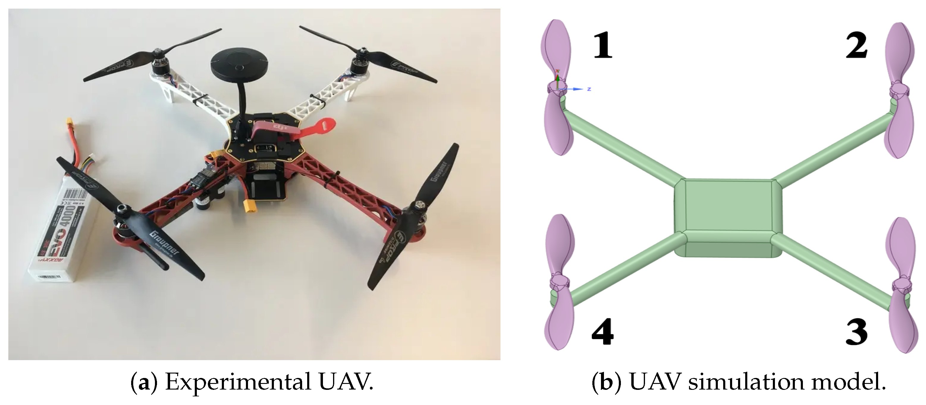
| Category | Frame | Control System | Blade | Electronic Speed Controller | Motor |
|---|---|---|---|---|---|
| Parameters | DJI F450 | Pixhawk 2.8.4 | 9450 Blade*4 | X-rotor 20A *4 | DIJ 2312S Brushless motor |
| Wind Sensor | Accuracy (RMSE) | |
|---|---|---|
| Speed (m/s) | Direction () | |
| DS-2 2D ultrasonic anemometer [30] | 0.27–0.67 m/s Under wind speed 1–5 m/s. | 25–56 Under wind speed 1–5 m/s. |
| Tri-Sonica Mini 2D ultrasonic anemometer [26] | 1.13 m/s Under wind speed 6.75 m/s. | 133.36 Under wind speed 6.75 m/s. |
| FT702 2D ultrasonic anemometer [33] | 0.6 m/s Under wind speed 11.0 m/s. | 12.0 Under wind speed 11.0 m/s. |
| Young Model 81000 ultrasonic anemometer [33] | 1.85 m/s | 113.67 |
| Tri-Sonica Mini [33] | 1.08 m/s | 87.05 |
| WPOD (this article) | 0.31 m/s in hovering position 0.73 m/s in moving position | 2.20 in hovering position 6.50 in moving position |
Disclaimer/Publisher’s Note: The statements, opinions and data contained in all publications are solely those of the individual author(s) and contributor(s) and not of MDPI and/or the editor(s). MDPI and/or the editor(s) disclaim responsibility for any injury to people or property resulting from any ideas, methods, instructions or products referred to in the content. |
© 2023 by the authors. Licensee MDPI, Basel, Switzerland. This article is an open access article distributed under the terms and conditions of the Creative Commons Attribution (CC BY) license (https://creativecommons.org/licenses/by/4.0/).
Share and Cite
Hou, T.; Xing, H.; Gu, W.; Liang, X.; Li, H.; Zhang, H. Wind Pressure Orthogonal Decomposition Anemometer: A Wind Measurement Device for Multi-Rotor UAVs. Drones 2023, 7, 366. https://doi.org/10.3390/drones7060366
Hou T, Xing H, Gu W, Liang X, Li H, Zhang H. Wind Pressure Orthogonal Decomposition Anemometer: A Wind Measurement Device for Multi-Rotor UAVs. Drones. 2023; 7(6):366. https://doi.org/10.3390/drones7060366
Chicago/Turabian StyleHou, Tianhao, Hongyan Xing, Wei Gu, Xinyi Liang, Haoqi Li, and Huaizhou Zhang. 2023. "Wind Pressure Orthogonal Decomposition Anemometer: A Wind Measurement Device for Multi-Rotor UAVs" Drones 7, no. 6: 366. https://doi.org/10.3390/drones7060366
APA StyleHou, T., Xing, H., Gu, W., Liang, X., Li, H., & Zhang, H. (2023). Wind Pressure Orthogonal Decomposition Anemometer: A Wind Measurement Device for Multi-Rotor UAVs. Drones, 7(6), 366. https://doi.org/10.3390/drones7060366