Article

Extraction and Mapping of Cropland Parcels in Typical Regions of Southern China Using Unmanned Aerial Vehicle Multispectral Images and Deep Learning

1
Guangdong Provincial Key Laboratory of Land Use and Consolidation, South China Agricultural University, Guangzhou 510642, China
2
College of Tropical Crops, Hainan University, Haikou 570100, China
*
Author to whom correspondence should be addressed.
Drones 2023, 7(5), 285; https://doi.org/10.3390/drones7050285
Submission received: 26 March 2023 / Revised: 19 April 2023 / Accepted: 21 April 2023 / Published: 24 April 2023
(This article belongs to the Special Issue Resilient UAV Autonomy and Remote Sensing)

Abstract

:
The accurate extraction of cropland distribution is an important issue for precision agriculture and food security worldwide. The complex characteristics in southern China pose great challenges to the extraction. In this study, for the objective of accurate extraction and mapping of cropland parcels in multiple crop growth stages in southern China, we explored a method based on unmanned aerial vehicle (UAV) data and deep learning algorithms. Our method considered cropland size, cultivation patterns, spectral characteristics, and the terrain of the study area. From two aspects—model architecture of deep learning and the data form of UAV—four groups of experiments are performed to explore the optimal method for the extraction of cropland parcels in southern China. The optimal result obtained in October 2021 demonstrated an overall accuracy (OA) of 95.9%, a Kappa coefficient of 89.2%, and an Intersection-over-Union (IoU) of 95.7%. The optimal method also showed remarkable results in the maps of cropland distribution in multiple crop growth stages, with an average OA of 96.9%, an average Kappa coefficient of 89.5%, and an average IoU of 96.7% in August, November, and December of the same year. This study provides a valuable reference for the extraction of cropland parcels in multiple crop growth stages in southern China or regions with similar characteristics.

1. Introduction

Cropland is the continuously managed land that is dedicated to growing crops [1]. It is essential for the global food security needed for human survival and production [2]. Cropland can produce food and other products that are essential for everyday life [3,4]. Therefore, cropland plays a key role in human activities. However, most existing cropland has been occupied or destroyed during the course of economic development, which has gradually begun to threaten the world’s food security, and thus there is an urgent need to protect cropland [5,6,7]. In the context of precision agriculture, accurate information regarding the spatial distribution of cropland is the foundation of cropland protection and a prerequisite for most agricultural efforts [8]. Accordingly, the accurate extraction of cropland is essential for global food security.
In southern China, croplands are always surrounded by scrub and woodland. The shape and size of cropland parcels differ from those characteristics in other regions of the country, as well as Europe and the United States [9]. The shapes of cropland parcels in southern China are mostly irregular, and the lengths of cropland parcel boundaries are mostly <80 m (some boundaries are <30 m). Various types of crops are often grown in adjacent cropland parcels, and occasionally more than one crop is grown in the same cropland parcel. In addition, crops in the cropland parcels could be in different phenological periods on the same date, and some cropland parcels may be bare land. Furthermore, the terrain of typical cropland in southern China is undulating, and many roads pass between cropland parcels. The roads are narrow, with widths of approximately 3–5 m. Overall, the characteristics of typical croplands in southern China are complex, which makes the extraction of cropland parcels challenging.
The satellite remote sensing technology has been widely employed in the extraction of cropland parcels. Various satellites, such as the Moderate-Resolution Imaging Spectroradiometer (MODIS) [10,11,12], Landsat [13,14,15,16], Satellite Pour l’Observation de la Terre (SPOT) [17,18], Sentinel [19,20,21,22], WorldView [23], and QuickBird [24], have achieved good results. Some studies have performed research in cropland extraction in southern China. The application of satellite data has achieved high precision. However, considering the challenges of cropland extraction in southern China and the limitation of the spatial resolution of satellite data, current satellite data are insufficient for accurate extraction. Therefore, data with higher spatial resolution are needed for the extraction of cropland parcels in southern China. In the past decade, unmanned aerial vehicles (UAVs) have been fitted with sensors that can collect images with very high spatial resolution. Thanks to the very high spatial resolution of UAV data, the more accurate extraction of cropland parcels can be satisfied in southern China.
The main methods for extracting cropland parcels from remote sensing data include object-oriented methods, traditional machine learning, and deep learning. The object-oriented method requires pre-segmentation of individual objects, which makes it challenging to determine the optimal segmentation scale in southern China, where the croplands are diverse in size [25,26,27]. In comparison to the object-oriented and the traditional machine learning methods, deep learning algorithms are capable of automatically extracting deep features, without the need for prior knowledge or additional artificial feature engineering [8,28]. Thus, in terms of efficiency and accuracy, deep learning algorithms have greater advantages in southern China.
There are scholars who utilize UAV data to extract croplands and other agricultural resources on small scales and complex features. Several studies have adopted the method of manual visual survey, employing UAV data with the highest spatial resolution they can afford, and visually delineating all cropland parcels [29,30]. However, this method will consume a lot of time, labor, and electrical energy, resulting in a low efficiency. There are studies experimenting with UAV images at different scales. For example, when performing cropland extraction, the spatial resolution of UAV data was modified, and different results were obtained. The extraction is found to be better when the spatial resolution is reduced. Such studies found that the accuracy of cropland extraction may be influenced by variations in the spatial resolution of UAV data [31,32]. However, such studies did not further explore the optimal spatial resolution, they only increased the diversity of data. The optimal spatial resolution needs to be explored for the cropland extraction in southern China to cope with the various sizes and shapes. In addition, some scholars have adopted the methods of object-oriented and machine learning (such as random forest and K-nearest neighbor), combined with auxiliary analysis (such as texture analysis and spectral analysis) methods [33,34]. This method firstly explores the optimal segmentation scale and subsequently segments various ground objects in the image based on the explored scale. Next, auxiliary features, such as spectral and texture features, are artificially selected, and finally, machine learning algorithms are employed to extract cropland. For instance, UAV digital images and the object-oriented method were employed for the extraction of cropland parcels. In such studies, texture, shape, and band information were analyzed as auxiliary features to improve the accuracy [35,36,37]. However, previous studies have mainly utilized spectral features as auxiliary data, with little exploration of more forms of fused data, such as various compositions of spectral bands and terrain information. The application of terrain information has provided a favorable auxiliary effect for the extraction of cropland [14,17,38]; thus, it is necessary to apply it in this study, especially in southern China, where the planting structure is complex, and the terrain is uneven. Furthermore, the artificial feature engineering in these studies requires additional time and high subjectivity, and it may be difficult to determine the object-oriented segmentation scale in southern China. Thus, with the object-oriented and machine learning methods, it may be difficult to fully extract the complex cropland features in southern China. There are also studies taking advantage of deep learning algorithms to extract cropland parcels from UAV data [39,40,41,42,43]. In the field of deep learning, the convolutional neural network (CNN) has shown outstanding results in the extraction of cropland parcels from UAV data due to its capacity in extracting the shape features of ground objects [44,45,46,47,48,49,50,51,52,53,54,55,56]. Among CNN algorithms, the U-Net-based model has gradually become one of the most popular models in the applications of precision agriculture due to the ability to recover object boundary information using the skip-connection in the decoder [57,58]. Nevertheless, most of the existing studies compare different types of CNN models or add auxiliary modules to the model, or change the optimizer to obtain different results, and few studies try to change the down-sampling architecture of the models to explore the optimal receptive field for specific ground objects. Therefore, the optimal down-sampling architecture of the model should be explored for more accurate extraction of cropland parcels in southern China. As mentioned above, the very high spatial resolution of UAV data presents great advantages in the application of cropland extraction. However, few studies have simultaneously explored the optimal extraction architecture of the model and the optimal data form (such as spatial resolution, spectral composition of bands, and terrain information fusion). In addition, most of the existing UAV-based extraction research utilizes single-period images, while in southern China, cropland has large spectral differences in different crop growth stages, so single-period image extraction studies may have poor robustness. Thus, it is necessary to explore the optimal method for accurate extraction of cropland parcels with multiple crop growth stages.
In summary, considering the challenges of cropland extraction in southern China, the potential of UAV data, and the advantages of deep learning, this study explores a method for accurate extraction of cropland parcels in southern China using very high spatial resolution UAV data deep learning algorithms. The main objective of this study is to explore the optimal method for accurate extraction of cropland parcels with multiple crop growth stages in southern China from the aspects of deep learning model architecture and the data form.

2. Materials and Methods

2.1. Selection of Study Area

An experimental station of South China Agricultural University, Guangzhou City, Guangdong Province, China, with some villages around, was selected as the study area (Figure 1a). Guangzhou belongs to the subtropical monsoon climate, characterized by cloudy and rainy weather throughout the year. There are three main types of soils: red soil, yellow soil, and paddy soil. Among them, red soil is the most common soil type, which has the characteristics of acidity, low phosphorus, low potassium, and low organic matter. Yellow soil has high fertility and good water permeability. Paddy soil has higher fertility and better water retention. The study area is surrounded by hills, and the terrain is undulating. The land use types in test sites were cropland, grassland, garden land, woodland, storage land, residential land, roads, and bodies of water. The cropland parcels in the test site were small, and some had an irregular shape. The area of cropland was much smaller than in the northern regions of China; additionally, the cropland parcel shape was mostly rectangular. The lengths and widths of typical cropland parcels were 65 × 35 m, 200 × 135 m, 85 × 50 m, 100 × 65 m, 130 × 45 m, 61 × 37 m, and 35 × 25 m. Diverse categories of crops were planted in different parcels. The crops grown in cropland parcels were rice, corn, soybeans, peanuts, pumpkins, vegetables, pepper, citrus, sugarcane, bananas, and dragon fruit. Most of the cropland parcels were covered with rice, corn, soybeans, and peanuts, and both rice and corn are biannual. The planting periods of typical crops in the study area can be seen in Figure 2. Within some non-conventional cropland parcels, many small areas of the field trials were locally constructed and were separated by concrete and plastic sheets. The concrete and plastic sheets caused some parcels to have local spectral characteristics that were similar to the characteristics of roads (Figure 1b–d). Large areas of woodland and scrub are distributed within the test site, and they have spectral characteristics similar to the cropland parcels. As mentioned above, the cropland features in this area are representative of the typical cropland features in southern China.

2.2. Data Acquisition and Preprocessing

In this study, a DJI Phantom 4 Multispectral quadrotor UAV (DJI Innovation Company Inc., Shenzhen, China) was used to collect data. The UAV carried six cameras (and the center wavelength of the single-band sensors): digital, blue band (450 ± 16 nm), green band (560 ± 16 nm), red band (650 ± 16 nm), red-edge band (730 ± 16 nm), and near-infrared band (840 ± 26 nm).
In order to achieve the purpose of extraction with multiple crop growth stages, the original data covered five temporal phases in the study area: August, September, October, November, and December 2021, which covered the complete key crop growth stages. To match the size of the study area to the endurance of the UAV battery, the UAV was set to fly at an altitude of 189 to 190 m, and the spatial resolution of the resulting data was 0.1 m. Additionally, the higher solar altitude angle between 11:00 and 13:00 would minimize shadow generation in the images, and therefore all original images were acquired during this time period. To ensure the quality of image mosaicking, the heading overlap rate and side-overlap rate were set to 75% and 70%, respectively. The flight speed was 8 m/s, the sensor lens was perpendicular to the ground, and the shooting time interval was 2 s. After the flight, the digital camera acquired the original images in joint photographic experts’ group (JPEG) format, and the other cameras obtained original images in tagged image file (TIF) format. In this study, we only used images in TIF format.
In addition to the sensor that receives the reflected light from the ground, the unmanned aerial vehicle (UAV) used in this study was equipped with a unique sensor that receives incident light intensity, allowing users to perform radiometric calibration without the need for a diffuse reflectance panel. According to the image processing guidelines of the DJI Phantom 4 Multispectral quadrotor UAV published by DJI Innovations, we performed radiometric correction on all bands of all collected raw images on a per-pixel basis. Thus, the raw image data underwent reflectance. The reflectance data were mosaicked through the Pix4DMapper software (Pix4D SA, Prilly, Switzerland). The acquired raw image data were mosaicked to obtain blue (B), green (G), red (R), red-edge (RE), and near-infrared (NIR) images of the study area, as well as a DSM raster map of the study area. The DSM was processed to obtain the slope raster map (Slope), and then the data were fused (the data fusion was directly added in this study). Two types of data were obtained from the data fusion. The first type was a fusion of B, G, R, RE, NIR, and DSM images to obtain multispectral fused data with DSM. The second type was a fusion of B, G, R, RE, NIR, and Slope images to obtain multispectral fused data with slope information. The initial spatial resolution of both types of fused data was 0.1 m.
To create the ground truth label used for model training, we first partially labeled the fused data according to the visual interpretation of the land categories. For land categories that could not be determined by visual interpretation, we conducted additional ground surveys to determine them. We formed polygons by drawing the boundaries of the land categories and assigned attributes to each polygon to label the land categories. Finally, we converted the labeled land category polygons into raster data as the ground truth labels for fused data.

2.3. Spectral Features of Data from UAV and Field Measurements

To better understand the spectral characteristics of the main types of ground objects in the study area, we collected ground spectral data for some parcels in mid-October when the crops were flourishing. The RS-8800 field spectroradiometer (Spectral Evolution, Haverhill, MA, USA) with a spectral range of 350–2500 nm and a spectral resolution of 1 nm was employed to measure the spectra of major crop types in cropland parcels and water bodies, respectively. Ten sample points were measured for each land category, and for crops, the canopy was measured and averaged, shown on a curve (Figure 3a). In addition, to compare the spectral information of ground measurements and the UAV images, we also collected 10 sample points in the UAV data for each main land category and the main crop in the cropland parcels, respectively, and calculated the mean and the confidence interval (CI) (Figure 3b,c).
According to the comparison between the spectral curves of measured data and the UAV image (Figure 3a,c), for most crops, there was a gradual increase in reflectance from the blue to the green band (450–560 nm), and peaks around the green band (560 nm). From the green to the red band (560–650 nm), the reflectance decreased and reached a valley around the red band (650 nm). In the range from the red to the near-infrared bands (650–840 nm), the reflectance continuously increased, and the increase from the red to the red-edge band (730 nm) was significantly higher than that from the red-edge to the near-infrared band.
In addition, it can be seen that the land categories within the study area had spectral diversity (Figure 3b). Water bodies exhibited higher reflectance in the green band compared to the other bands, with the lowest reflectance observed in the near-infrared band. Overall, the reflectance was always low from the blue to the near-infrared band, without a significant increase, and remained below 20%. The reflectance of constructions and roads was also relatively stable across all bands of the UAV, and was higher than that of water bodies, with little variation. Additionally, the reflectance of constructions and roads was higher than that of vegetation in the visible band, and lower in the red-edge and near-infrared bands. Forests and shrubs had similar spectral curves to the vegetation in cropland; especially, forests occupied a large area in the study area, and shrubs were distributed along roads between cropland parcels. Moreover, the reflectance of forests and shrubs (and other vegetation) exhibited more distinct variations across different bands compared to water bodies, constructions, and roads. Thus, it will be a great challenge to distinguish forests and shrubs from cropland in this study.
It can be seen that for the corresponding land category, the spectral features presented by UAV data and ground spectral data had the same regularity. Therefore, the UAV data collected in this study had high reliability.

2.4. Deep Learning Algorithms

U-Net-based CNN algorithms
Since the U-Net-based convolutional neural network (CNN) has been proven to obtain better extraction results with limited training samples, this study utilized the U-Net model as the basis for the experiments. The U-Net model (Figure 4a) is an end-to-end network model proposed by Ronneberger et al. for image segmentation [57]. The U-Net model is proposed for image segmentation tasks, as it effectively combines high-level semantic information from the encoding path with detailed information from the decoding path. The symmetrical architecture also enables the model to have a large number of trainable parameters, allowing it to capture deep information from the input images.
U-Net++ (Figure 4b) is a variant of the U-Net model [59], which was proposed to overcome some of the limitations of the original U-Net. The main improvement of the U-Net++ model lies in the encoding and decoding paths. The U-Net++ introduces the concept of nested U-Net architecture and dense blocks, which allow it to better-capture the multi-scale context information from input images, resulting in improved performance for the applications in image segmentation.
Since this study is a small-scale study with a small number of samples, U-Net and U-Net++ models were employed as the basic network models for the experiments.
Model training
In model training, the training dataset is used to train the model, while the validation dataset is used to evaluate the performance of the model during training. During the training process, the model is iteratively trained using the training dataset and its performance is evaluated using the validation dataset. The feedback from the validation dataset allows the model to make changes that are beneficial for improving the accuracy during iterations on the training dataset. This process continues until the model achieves satisfactory results on the validation dataset.
When training the model, all pixel values of images were normalized into the range of [0, 1] before they were input into the CNN model. Table 1 shows the related parameters of model training. Weight parameters were saved after each epoch during model training.
Considering the deep learning algorithms and GPU memory limitations, the ground truth labels overlapped with all multispectral fused data (5 temporal phases) were cropped into slices consisting of 256 × 256 pixels. A total of 2444 slices, each consisting of 256 × 256 pixels, were randomly shuffled and input into the training model, which was then divided into a training dataset (1952 slices) and a validation dataset (492 slices) in a 4:1 ratio. The training dataset was used to guide the accuracy adjustment. The validation dataset was used to assess the training performance of each algorithm.

2.5. Experiment Design

To explore the optimal method for accurate extraction of cropland parcels with multiple crop growth stages, a general experimental framework was designed (Figure 5). The UAV data of five phases were collected to ensure multiple crop growth tests. According to the characteristics of the study area, four groups of comparison experiments investigating four factors (CNN architecture, spatial resolution, spectral band composition, and terrain information) were successively carried out in this study. The optimal parameters in each group of experiments were used as the basis for the next group of experiments. Finally, the optimal overall method was obtained and applied to multiple crop growth stages.

2.5.1. Exploration of Optimal Network Architecture

Distinct extraction tasks require diverse receptive fields. The down-sampling architecture of a convolutional neural network serves as a key determinant of receptive fields. In order to explore the optimal U-Net-based convolutional neural network architecture for achieving the objective of this study, a group of experimental comparisons were performed (experiment group A).
We first extracted cropland parcels using the original U-Net model, then made modifications to the original U-Net network architecture to explore the effects of network architecture complexity. We also modified the U-Net++ model and compared it with different modified forms of the U-Net model. The specific experimental code and the comparisons are shown in Table 2.

2.5.2. Exploration of Optimal Spatial Resolution

In previous studies, almost no study explored the optimal spatial resolution for a specific task. Moreover, due to the unique scale of typical cropland in southern China, it is more necessary to explore the optimal spatial resolution. In order to explore the optimal spatial resolution of the data for the objective of this study, based on the optimal network architecture identified in Section 2.5.1, the preprocessed multispectral data were resampled to generate data with various spatial resolutions. A group of experimental comparisons were performed (experiment group B). The specific experimental code and the comparisons are shown in Table 3.

2.5.3. Exploration of Optimal Spectral Composition

Typical features in the study area include cropland, woodland, scrub, water bodies, and roads. The spectral characteristics of cropland in the study area are complex, and numerous other vegetation types have similar spectral characteristics. Cropland, woodland, and scrub consist mainly of vegetation with similar spectral characteristics. In cropland parcels, rice, corn, soybean, and peanut are mainly planted. The complex planting structure may lead to complex spectral characteristics within the cropland category. Therefore, it is necessary to explore the impact of different spectral compositions of the data and investigate the optimal spectral composition in this study.
In order to explore the optimal spectral composition of the data for the objective of this study, based on the optimal network architecture and spatial resolution in Section 2.5.2, fused data for different spectral compositions were established, and a group of experimental comparisons were performed (experiment group C). Their spectral compositions are shown in Table 4.

2.5.4. The Terrain Information Fusion Exploration

Due to the unevenness in southern China, cropland areas tend to have an undulating terrain. Terrain information such as DEM and DSM have been fused with data in previous extraction tasks and improved the results. To achieve the objective of this study, it is necessary to explore the optimal terrain information fusion of the dataset. Based on the optimal network architecture, the optimal spatial resolution, and the best-performing spectral composition in Section 2.5.3, multiple groups of data with different terrain information were used in a group of experimental comparisons (experiment group D). The specific experimental code and the comparisons are shown in Table 5. It is worth noting that this study employed slope information, which has rarely been employed in existing studies based on UAV data.
Finally, to test the robustness of multiple crop growth stages, fusion data slices from August, November, and December 2021 were selected, and the optimal method in Section 2.5.4 was applied for testing.

2.6. Accuracy Assessment

To evaluate the result of each experiment, during the experiments, we randomly split the data to be input into the training network model into a training dataset and a validation dataset. The training dataset was used to guide the accuracy adjustment. The validation dataset was used to assess the training performance of each algorithm. Another temporal phase of the fused data (test dataset) was used to explore the results of the models in each experiment. The fused data slices of September 2021 in the study area were selected and divided into a training dataset and a validation dataset at a ratio of 4:1. The fused data slices of the whole study area in October 2021 were selected as the test dataset.
A confusion matrix was created to evaluate the experimental results in this study. Based on the confusion matrix, we used three common indicators of deep learning (Overall accuracy (OA), Kappa coefficient, and Intersection-over-Union (IoU)) to evaluate the effect of cultivated land extraction.
The OA was calculated as follows (Equation (1)):
O A = T P + T N T P + T N + F P + F N
where T P is the number of pixels of true positives, T N is the number of pixels of true negatives, F P is the number of pixels of false positives, and F N is the number of pixels of false negatives. A “positive” result was where the model predicted that the pixels were cropland, whereas a “negative” result was where the model predicted that the pixels were non-cropland (background). A true or false status was dependent on whether the prediction was consistent with the ground truth label.
The Kappa coefficient was calculated as follows (Equation (2)):
K a p p a = O A p e 1 p e
where N and p e were calculated as follows:
p e = a 0 × b 0 + a 1 × b 1 N 2
N = T P + F P + T N + F N
In Equations (3) and (4), a 0 and a 1 are the numbers of pixels of non-cropland and cropland in the ground truth label, respectively, and b 0 and b 1 are the numbers of pixels of non-cropland and cropland predicted by the model, respectively.
The IoU was calculated as follows (Equation (5)):
I o U = T P T P + F P + F N

3. Results and Analysis

For the objective of exploration of the optimal method for accurate extraction of cropland parcels on multiple crop growth stages in southern China, in this section, we present the experiment results with respect to test dataset evaluation by the trained models.

3.1. Analysis of U-Net-Based CNN Architecture

The accuracy assessment of experiment results and the maps extracted from the test dataset are shown in Table 6 and Figure 6, respectively.
According to the experiment results, the performance of the original U-Net model (A1) was poor, with many incorrect extractions for forest, scrub, and roads. After network deepening, several improved models based on the U-Net model all achieved better results than the original U-Net model. A U-Net model with one additional layer of down-sampling (A2) was the best modified U-Net model, with an OA of 89.9%, a Kappa coefficient of 74.5%, and an IoU of 89.6%. These were respective improvements of 6.2%, 7.6%, and 6.5% over the original U-Net model. Model A2 significantly reduced the incorrect extractions for non-cropland vegetation. After the complexity of the network model was further increased (models A3 and A4), the assessment indicators gradually decreased, and the incorrect extraction of non-cropland ground features gradually increased.
The original U-Net++ model (A5) and the modified U-Net++ model (A6) achieved better results than all U-Net models used in this study. The original U-Net++ model (A5) achieved an OA of 91.3%, a Kappa coefficient of 78.7%, and an IoU of 91.1%, while the modified U-Net++ model was less effective than the original U-Net++ model, with an OA of 90.4%, Kappa coefficient of 76.6%, and an IoU of 90.2%, respectively. The prediction results of the two U-Net++-based models implied that both had fewer missing extractions for cropland parcels and fewer incorrect extractions for non-cropland, compared with all U-Net-based models. Although the modified U-Net++ model (A6) produced some incorrect extractions for roads, the original U-Net++ model (A5) performed well. The original U-Net++ model (A5) achieved the best result in this group of experiments.
These results indicated that the U-Net model could learn deeper features in the training process when the number of network layers was appropriately increased or the network architecture became more complex, thereby improving the model. However, the optimal number of layers of the network model was not the highest number possible. In a particular segmentation task, after the number of network layers reached the optimum, further increases would weaken the model performance, although this model was initially expected to be better than the original model.
In the experiments, various modified forms of the U-Net model produced worse predictions than the U-Net++ model based on the test dataset (A5), which confirmed that the conclusion of the creators of U-Net++ (i.e., “the U-Net++ model is always better than the U-Net model”) was applicable to this study. When we attempted to expand the size of the pooling kernel of the U-Net++ model from 2 × 2 to 4 × 4 (A4, equivalent to increasing its degree of down-sampling), the predictive effect of the trained model on the test dataset was better than the predictive effect of the improved architecture of all U-Net models, but it was less robust than the original U-Net++ model (A5). This situation presumably occurred because the original U-Net++ model extracted better features when fusing the output feature maps of different sizes. The receptive field of the model might be further increased when the pooling kernel size and pooling stride are expanded, leading to a weakened U-Net++ model performance.
Although the original U-Net++ model (A5) demonstrated a significantly better performance than the other models in the experiments, the accuracy assessments of the experiments revealed that all trained models in this group of experiments only predicted a Kappa coefficient of 60–80% for the test dataset. The Kappa coefficient of the U-Net++ model (A5) with the best result in this group of experiments did not reach 80%. Although the model produced a nearly complete extraction of cropland parcels, more non-cropland areas were incorrectly extracted into cropland. Most of the incorrectly extracted non-cropland areas were woodland, roadside shrubs, and hillsides, where weeds and trees were distributed. The incorrect extraction may have occurred because the contiguous vegetation had spectra similar to the spectra of crops within the cropland, and the spatial resolution of the data was excessively high (0.1 m). Due to the obvious ridges in some cropland parcels in the study area and the presence of mulching film on the ground around the crops, the spectral composition in the cropland parcels was complex. Therefore, the very high spatial resolution increased the difficulty of extraction. The spatial resolution needs to be decreased and the optimal spatial resolution needs to be explored to reach the objective of this study.

3.2. Analysis of Different Spatial Resolution

In previous studies concerning the use of UAVs combined with remote sensing, researchers usually adopted the highest possible spatial resolution (≤0.05 m) according to the cost. However, when completing a specific extraction, few researchers have explored the optimal spatial resolution of data specific to their task. Although numerous researchers have achieved generally good results in extraction tasks using spatial resolutions of <0.05 m, most of their study objects had obvious spectral and shape features, and the non-target objects were not sufficiently intrusive. Examples include the extraction of carrots, greenhouses with mulch, citrus trees, vegetables, lodged rice, and individual plant species.
Based on the optimal network architecture (A5) in the experiment group A, the spatial resolutions of input data were resampled into 0.3, 0.4, 0.5, 0.6, 0.7, 0.8, 0.9, and 1.0 m. The resampled data were input into the U-Net++ network and trained accordingly for the experiment group B. The accuracy assessment of experiment results and the maps extracted from the test dataset are shown in Table 7, as well as Figure 7 and Figure 8.
The accuracy assessment of experiment results showed that the 0.5 m dataset (B3) had the best result, with an OA of 94.5%, a Kappa coefficient of 85.6%, and an IoU of 94.4%. These represented respective increases of 3.2%, 6.5%, and 3.3%, compared with the 0.1 m dataset before resampling. The maps showed that outstanding results were achieved at spatial resolutions of 0.5 m (B3) and 0.8 m (B6). The accuracy assessment, as well as the local details, showed the best results for the 0.5 m dataset. According to the maps, when the spatial resolution decreased, the results of the extraction clearly improved, and the incorrect extraction of non-cropland features decreased. The spatial resolutions of 0.3, 0.6, and 0.7 m all tended to incorrectly extract some forested and weed-covered slopes into cropland. The spatial resolutions of 0.1 and 1.0 m had the worst results. Overall, these findings indicated that the enhancement of spatial resolution over a certain range could improve the effectiveness of the model for cropland extraction, but the effectiveness of the model worsened when the spatial resolution became excessively high.
Spatial resolutions of 0.5 and 0.8 m achieved similar overall results, which were better than the other spatial resolutions, but the 0.5 m dataset performed better in terms of the smoothness and completeness of cropland parcels, compared with the 0.8 m dataset. The 0.8 m dataset incorrectly extracted some narrow field roads into cropland. The 0.5 m dataset almost completely retained roads located in the fields.

3.3. Results of Different Spectral Compositions

The experiment group C was performed based on the optimal result of the experiment group B (U-Net++ CNN architecture and 0.5 m spatial resolution dataset). Datasets of different spectral compositions were used for the experiments. The accuracy assessment of experiment results and the maps extracted from the test dataset of experiment group C are shown in Table 8, as well as Figure 9 and Figure 10.
The accuracy assessment showed that an RGB-RE-NIR-fused multispectral dataset (C4) achieved the best result, with an OA of 95.6%, a Kappa coefficient of 88.5%, and an IoU of 95.5%. The results were similar for the RGB-only dataset (C1) and the RGB-NIR-fused multispectral dataset (C3). The maps showed that RGB images (C1) and RGB-RE-NIR-fused images (C4) achieved better results than RGB-RE-fused images (C2) and RGB-NIR-fused images (C3). The results of RGB-RE-fused images (C2) were generally poor. The local prediction details showed that RGB-RE-NIR-fused images (C4) more fully extracted cropland parcels and exhibited better performance in extracting fragmented cropland parcels, compared with RGB images (C1).
When RGB images were used to fuse the RE band (C2) or the NIR band (C3), the experimental results were worse than when RGB images were used alone. However, in this study, although greater interference was caused by vegetation, the fusion of RGB images with both RE and NIR bands (C4) resulted in deeper interference features and more distinctly different crops within the cropland parcels, which improved the model performance. Although many researchers presume that the RE band makes a positive contribution to the analysis of vegetation, our experiments indicated that the RGB-RE-fused images (C2) were less effective, which suggests that the RE band alone may not be appropriate for the extraction of typical cropland parcels in southern China.

3.4. Analysis on Fusion of Terrain Information

Previous studies have shown that the fusion of terrain information into images can improve the models’ performance. For example, when DSM and RGB images were combined in a land cover classification and the classification results were compared with RGB-only images, the results of RGB-DSM-integrated images were better than the results of RGB-only images.
The experiment group D was performed based on the U-Net++ model and RGB-RE-NIR-fused images, with 0.5 m spatial resolution. Images fused with different terrain information were trained. The accuracy assessment of experiment results and the maps extracted from the test dataset of experiment group D are shown in Table 9, as well as Figure 11 and Figure 12.
The accuracy assessment revealed that the use of terrain information yielded better results compared with the lack of terrain information. Slope fusion with RGB-RE-NIR images (D3) achieved the best result, with an OA of 95.9%, a Kappa coefficient of 89.1%, and an IoU of 95.7%. The OA, Kappa coefficient, and IoU of DSM fusion with RGB-RE-NIR images (D1) were 95.6%, 88.5%, and 95.5%, respectively, which were slightly worse than the results for slope fusion with RGB-RE-NIR images (D3). Although similar overall results were obtained for the three experiments, the slope fusion with RGB-RE-NIR images (D3), which extracted cropland parcels with fewer omissions, produced the best results in terms of local prediction details.
There were also very few parcels within which high protective shelters had been erected for local crops, which made them significantly taller than the surrounding parcels. The extraction model was likely to misjudge the DSM information. The result of slope data fused with multispectral data (D3) was clearly better than the result of the DSM. This is presumably because the study area was located in southern China, where the terrain is not generally flat, and this characteristic hinders the process of DSM-fused data training. However, the slope of most cropland parcels was similar, and varied over a small range. Therefore, the data fused with the slope achieved better results in the typical cropland regions of southern China.

4. Discussion

4.1. Comparison to Previous Studies

In this study, a method for accurate extraction of cropland parcels in southern China on multiple crop growth stages was explored. The main contribution of this study is exploring the optimal method from the aspects of deep learning model architecture and the UAV data form. The optimal U-Net-based model architecture, spatial resolution of data, spectral composition, and fusion of terrain information were explored based on four experiment groups. Finally, the robustness of the method was tested by the application on more crop growth stages.
In terms of CNN architecture, the existing studies have mainly focused on the comparison of different models and the improvement of the models (such as adding attention mechanisms in the models) [46]. We explored the receptive field suitable for this study by changing the down-sampling architecture of the model, which was rarely covered in previous studies. In terms of spatial resolution, some existing studies utilized the highest spatial resolution they could afford [32]. However, the specific characteristics of the study area should be taken into consideration. Cropland in southern China has more complex image features because of the complex planting structure and distribution. To maximize the advantages of UAV data, we resampled original UAV data into different spatial resolutions and explored the optimal one. In terms of the form of data fusion, the experiments found different results from existing studies. Although some existing studies suggest that the RE band has a greater role in agricultural applications [60], we found that fusing only the RE band with RGB data had a relatively poor result in southern China. Additionally, based on the findings of existing studies on the role of the DSM, we explored the fusion of different terrain information. The slope data, which has barely been employed in previous studies, was fused with the multispectral dataset in this study. The experimental results indicate that the slope data were more suitable for southern China than the DSM. The exploration of spectral combination and terrain information helped identify the most suitable form of UAV data for cropland extraction in southern China.
In addition, in order to test the robustness, the optimal method for accurate extraction of cropland parcels in southern China explored in this study was applied to test datasets collected in more periods (in August, November, and December). The accuracy assessment of results and the maps extracted are shown in Table 10 and Figure 13.
According to the accuracy assessment, the method achieved a similar accuracy to experiment D3 when it was applied to other periods. The maps presented the good robustness of the method, particularly when applying to datasets collected in August and November.
The method explored in this study can be utilized for cropland extraction in multiple crop growth stages in southern China and regions with similar characteristics (such as some areas in Southeast Asia with severe cropland fragmentation and complex planting structures).

4.2. Uncertainties

There were some deficiencies in the results. First, there were some omissions in the extraction results (in the west of the maps). This is presumably because within some non-conventional cropland parcels, many small areas of the field trials were locally constructed and were separated by concrete and plastic sheets. The concrete and plastic sheets caused some parcels to have local spectral characteristics that were similar to the characteristics of roads.
In addition, in the map extracted from the test dataset collected in December, some small holes appeared in some cropland parcels. These holes may be due to the fact that some parcels had been harvested and were in the state of bare soil with fewer weeds during this period. The dataset employed for training was collected in September, when almost no cropland parcels were in the bare soil state. Therefore, the holes in the extraction results from December may be because the model only used the boundary and the contextual information of cropland parcels.
Additionally, due to the impact of the COVID-19 pandemic, field operations have been restricted, especially with strict controls over flight zones, and the continuous outbreak of the La Nina phenomenon in 2022 has brought prolonged rainy and typhoon weather to southern China, resulting in a failure to collect datasets with longer timespans to further test the robustness of this method for multiple crop growth stages.

4.3. Implications and Future Work

The quantity of cropland in China has sharply decreased because of economic development and the promotion of urbanization and industrialization, particularly in the well-developed economic region of southern China. Thus, there is a need to protect cropland and ensure food security [61,62]. Cropland has complex features in southern China, which makes it difficult to accurately extract data from images used to support precision agriculture. The accurate extraction and mapping of cropland parcels will help the Departments of Natural Resources and Agriculture to manage and protect cropland in a more systematic manner, thereby improving food security nationwide [63].
This study had some limitations that can be improved in future work. First, we did not explore whether the reduction of the U-Net++ model’s complexity would lead to better extraction of cropland parcels. Second, this study did not explore other advanced network models in the field of semantic segmentation (e.g., fully convolutional networks, SegNet, and the DeeplabV3 series). In the future, we will investigate different spatial resolutions when using different models to determine whether the selection of optimal spatial resolution is relevant for different types of network models. We will also attempt to apply our method to other cropland regions which have similar features to southern China. Finally, we will explore combining WorldView data (the spatial resolutions of WorldView-3 and WorldView-4 are 0.31 m for panchromatic images and 1.24 m for multispectral images) with UAV data, then applying these data to our method.

5. Conclusions

In this study, for the objective of accurate extraction of cropland parcels with multiple crop growth stages in southern China, we explored a method based on unmanned aerial vehicle (UAV) data and deep learning algorithms.
The multispectral UAV data were collected and preprocessed. The U-Net and U-Net++ models, along with some of their modified forms, were adopted to perform the experiments. An experimental station in Guangzhou, China, was selected to represent a typical region in southern China. Datasets from different periods were separately trained and tested. Our results showed that the optimal method for extraction of typical cropland parcels in multiple crop growth stages in southern China was an RGB-RE-NIR-slope-fused dataset, with a spatial resolution of 0.5 m and trained with the U-Net++ model. This method achieved an average OA of 96.9%, an average Kappa coefficient of 89.5%, and an average IoU of 96.7% for the test dataset in various crop growth stages.
The method explored in this study provides a theoretical method for accurate extraction of cropland parcels in multiple crop growth stages in typical cropland regions of southern China and other similar areas, such as some areas in Southeast Asia, where cropland fragmentation and complex planting structures are prevalent.

Author Contributions

Conceptualization, L.L. and S.W.; methodology, L.L. and S.W.; software, L.L.; validation, S.W., Y.S. and H.X.; formal analysis, S.W., X.L. and Y.S.; investigation, X.L.; resources, S.W., H.X., X.L., S.K., B.Z. and Y.H.; data curation, S.W. and L.L.; writing—original draft preparation, S.W.; writing—review and editing, S.W., Y.S., H.X., X.L., S.K., B.Z. and L.L.; visualization, S.W.; supervision, S.W. and L.L.; project administration, L.L. and Y.H. All authors have read and agreed to the published version of the manuscript.

Funding

This work was supported by the National Natural Science Foundation of China (grant number U1901601) and the National Key Research and Development Program of China (grant number 2020YFD1100203).

Data Availability Statement

Not applicable.

Acknowledgments

The authors want to thank the editor, associate editor, and anonymous reviewers for their helpful comments and advice.

Conflicts of Interest

The authors declare no conflict of interest.

References

  1. Liu, J.; Liu, M.; Tian, H.; Zhuang, D.; Zhang, Z.; Zhang, W.; Tang, X.; Deng, X. Spatial and Temporal Patterns of China’s Cropland during 1990–2000: An Analysis Based on Landsat TM Data. Remote Sens. Environ. 2005, 98, 442–456. [Google Scholar] [CrossRef]
  2. Lai, Z.; Chen, M.; Liu, T. Changes in and Prospects for Cultivated Land Use since the Reform and Opening up in China. Land Use Policy 2020, 97, 104781. [Google Scholar] [CrossRef]
  3. Davis, S.C.; Anderson-Teixeira, K.J.; DeLucia, E.H. Life-Cycle Analysis and the Ecology of Biofuels. Trends Plant Sci. 2009, 14, 140–146. [Google Scholar] [CrossRef] [PubMed]
  4. Wilkins, T.A.; Rajasekaran, K.; Anderson, D.M. Cotton Biotechnology. Crit. Rev. Plant Sci. 2000, 19, 511–550. [Google Scholar] [CrossRef]
  5. Song, W.; Pijanowski, B.C. The Effects of China’s Cultivated Land Balance Program on Potential Land Productivity at a National Scale. Appl. Geogr. 2014, 46, 158–170. [Google Scholar] [CrossRef]
  6. Wang, L.; Zheng, W.; Tang, L.; Zhang, S.; Liu, Y.; Ke, X. Spatial Optimization of Urban Land and Cropland Based on Land Production Capacity to Balance Cropland Protection and Ecological Conservation. J. Environ. Manag. 2021, 285, 112054. [Google Scholar] [CrossRef]
  7. Wu, Y.; Shan, L.; Guo, Z.; Peng, Y. Cultivated Land Protection Policies in China Facing 2030: Dynamic Balance System versus Basic Farmland Zoning. Habitat Int. 2017, 69, 126–138. [Google Scholar] [CrossRef]
  8. Xia, L.; Luo, J.; Sun, Y.; Yang, H. Deep Extraction of Cropland Parcels from Very High-Resolution Remotely Sensed Imagery. In Proceedings of the 2018 7th International Conference on Agro-Geoinformatics (Agro-Geoinformatics), Hangzhou, China, 6–9 August 2018; pp. 1–5. [Google Scholar]
  9. Niu, Z.; Yan, H.; Liu, F. Decreasing Cropping Intensity Dominated the Negative Trend of Cropland Productivity in Southern China in 2000–2015. Sustainability 2020, 12, 10070. [Google Scholar] [CrossRef]
  10. Chen, Y. Mapping Croplands, Cropping Patterns, and Crop Types Using MODIS Time-Series Data. Int. J. Appl. Earth Obs. Geoinf. 2018, 69, 133–147. [Google Scholar] [CrossRef]
  11. Wu, Z.; Thenkabail, P.S.; Mueller, R.; Zakzeski, A.; Melton, F.; Johnson, L.; Rosevelt, C.; Dwyer, J.; Jones, J.; Verdin, J.P. Seasonal Cultivated and Fallow Cropland Mapping Using MODIS- Based Automated Cropland Classification Algorithm. J. Appl. Remote Sens. 2014, 8, 18. [Google Scholar] [CrossRef]
  12. Xiong, J.; Thenkabail, P.S.; Gumma, M.K.; Teluguntla, P.; Poehnelt, J.; Congalton, R.G.; Yadav, K.; Thau, D. Automated Cropland Mapping of Continental Africa Using Google Earth Engine Cloud Computing. ISPRS J. Photogramm. Remote Sens. 2017, 126, 225–244. [Google Scholar] [CrossRef]
  13. Dimov, D.; Löw, F.; Ibrakhimov, M.; Conrad, C. Feature Extraction and Machine Learning for the Classification of Active Cropland in the Aral Sea Basin. In Proceedings of the 2017 IEEE International Geoscience and Remote Sensing Symposium (IGARSS), Fort Worth, TX, USA, 23–28 July 2017; pp. 1804–1807. [Google Scholar]
  14. Teluguntla, P.; Thenkabail, P.S.; Oliphant, A.; Xiong, J.; Gumma, M.K.; Congalton, R.G.; Yadav, K.; Huete, A. A 30-m Landsat-Derived Cropland Extent Product of Australia and China Using Random Forest Machine Learning Algorithm on Google Earth Engine Cloud Computing Platform. ISPRS J. Photogramm. Remote Sens. 2018, 144, 325–340. [Google Scholar] [CrossRef]
  15. Xu, H.; Xiao, X.; Qin, Y.; Qiao, Z.; Long, S.; Tang, X.; Liu, L. Annual Maps of Built-Up Land in Guangdong from 1991 to 2020 Based on Landsat Images, Phenology, Deep Learning Algorithms, and Google Earth Engine. Remote Sens. 2022, 14, 3562. [Google Scholar] [CrossRef]
  16. Su, Y.; Wu, S.; Kang, S.; Xu, H.; Liu, G.; Qiao, Z.; Liu, L. Monitoring Cropland Abandonment in Southern China from 1992 to 2020 Based on the Combination of Phenological and Time-Series Algorithm Using Landsat Imagery and Google Earth Engine. Remote Sens. 2023, 15, 669. [Google Scholar] [CrossRef]
  17. Duro, D.C.; Franklin, S.E.; Dubé, M.G. A Comparison of Pixel-Based and Object-Based Image Analysis with Selected Machine Learning Algorithms for the Classification of Agricultural Landscapes Using SPOT-5 HRG Imagery. Remote Sens. Environ. 2012, 118, 259–272. [Google Scholar] [CrossRef]
  18. Deng, J.; Wang, K.; Shen, Z.; Xu, H. Decision tree algorithm of automatically extracting farmland information from SPOT-5 images based on characteristic bands. Trans. Chin. Soc. Agric. Eng. 2004, 20, 145–148. [Google Scholar]
  19. Belgiu, M.; Csillik, O. Sentinel-2 Cropland Mapping Using Pixel-Based and Object-Based Time-Weighted Dynamic Time Warping Analysis. Remote Sens. Environ. 2018, 204, 509–523. [Google Scholar] [CrossRef]
  20. Csillik, O.; Belgiu, M. Cropland Mapping from Sentinel-2 Time Series Data Using Object-Based Image Analysis. In Proceedings of the 20th AGILE International Conference on Geographic Information Science Societal Geo-Innovation Celebrating, Wageningen, The Netherlands, 9 May 2017; pp. 9–12. [Google Scholar]
  21. Useya, J.; CHEN, S. Exploring the Potential of Mapping Cropping Patterns on Smallholder Scale Croplands Using Sentinel-1 SAR Data. Chin. Geogr. Sci. 2019, 29, 626–639. [Google Scholar] [CrossRef]
  22. Valero, S.; Morin, D.; Inglada, J.; Sepulcre, G.; Arias, M.; Hagolle, O.; Dedieu, G.; Bontemps, S.; Defourny, P.; Koetz, B. Production of a Dynamic Cropland Mask by Processing Remote Sensing Image Series at High Temporal and Spatial Resolutions. Remote Sens. 2016, 8, 55. [Google Scholar] [CrossRef]
  23. McCarty, J.L.; Neigh, C.S.R.; Carroll, M.L.; Wooten, M.R. Extracting Smallholder Cropped Area in Tigray, Ethiopia with Wall-to-Wall Sub-Meter WorldView and Moderate Resolution Landsat 8 Imagery. Remote Sens. Environ. 2017, 202, 142–151. [Google Scholar] [CrossRef]
  24. Xu, W.; Zhang, G.; Huang, J. An Object-Oriented Approach of Extracting Special Land Use Classification by Using Quick Bird Image. In Proceedings of the IGARSS 2008–2008 IEEE International Geoscience and Remote Sensing Symposium, Boston, MA, USA, 7–11 July 2008; pp. IV-727–IV-730. [Google Scholar]
  25. Cai, Z.; Hu, Q.; Zhang, X.; Yang, J.; Wei, H.; He, Z.; Song, Q.; Wang, C.; Yin, G.; Xu, B. An Adaptive Image Segmentation Method with Automatic Selection of Optimal Scale for Extracting Cropland Parcels in Smallholder Farming Systems. Remote Sens. 2022, 14, 3067. [Google Scholar] [CrossRef]
  26. Wen, C.; Lu, M.; Bi, Y.; Zhang, S.; Xue, B.; Zhang, M.; Zhou, Q.; Wu, W. An Object-Based Genetic Programming Approach for Cropland Field Extraction. Remote Sens. 2022, 14, 1275. [Google Scholar] [CrossRef]
  27. Xu, L.; Ming, D.; Zhou, W.; Bao, H.; Chen, Y.; Ling, X. Farmland Extraction from High Spatial Resolution Remote Sensing Images Based on Stratified Scale Pre-Estimation. Remote Sens. 2019, 11, 108. [Google Scholar] [CrossRef]
  28. Xu, W.; Deng, X.; Guo, S.; Chen, J.; Sun, L.; Zheng, X.; Xiong, Y.; Shen, Y.; Wang, X. High-Resolution U-Net: Preserving Image Details for Cultivated Land Extraction. Sensors 2020, 20, 4064. [Google Scholar] [CrossRef]
  29. Yu, K.; Shan, J.; Wang, Z.; Lu, B.; Qiu, L.; Mao, L. Land use status monitoring in small scale by unmanned aerial vehicles (UAVs) observations. Jiangsu J. Agric. Sci. 2019, 35, 853–859. [Google Scholar]
  30. Wang, Y.; Zhang, Y.; Men, L.; Liu, B. UAV survey in the third national land survey application of pilot project in Gansu. Geomat. Spat. Inf. Technol. 2019, 42, 219–221. [Google Scholar]
  31. Johansen, K.; Raharjo, T.; McCabe, M. Using Multi-Spectral UAV Imagery to Extract Tree Crop Structural Properties and Assess Pruning Effects. Remote Sens. 2018, 10, 854. [Google Scholar] [CrossRef]
  32. Xi, X.; Xia, K.; Yang, Y.; Du, X.; Feng, H. Urban individual tree crown detection research using multispectral image dimensionality reduction with deep learning. Natl. Remote Sens. Bull. 2022, 26, 711–721. [Google Scholar]
  33. Breiman, L. Random Forests. Mach. Learn. 2001, 45, 5–32. [Google Scholar] [CrossRef]
  34. Cortes, C.; Vapnik, V. Support-Vector Networks. Mach Learn 1995, 20, 273–297. [Google Scholar] [CrossRef]
  35. Hu, X.; Li, X.; Min, X.; Niu, B. Optimal Scale Extraction of Farmland in Coal Mining Areas with High Groundwater Levels Based on Visible Light Images from an Unmanned Aerial Vehicle (UAV). Earth Sci. Inform. 2020, 13, 1151–1162. [Google Scholar] [CrossRef]
  36. Xu, W.; Lan, Y.; Li, Y.; Luo, Y.; He, Z. Classification Method of Cultivated Land Based on UAV Visible Light Remote Sensing. Int. J. Agric. Biol. Eng. 2019, 12, 103–109. [Google Scholar] [CrossRef]
  37. Zhang, C.; Wei, S.; Ji, S.; Lu, M. Detecting Large-Scale Urban Land Cover Changes from Very High Resolution Remote Sensing Images Using CNN-Based Classification. ISPRS Int. J. Geo-Inf. 2019, 8, 189. [Google Scholar] [CrossRef]
  38. Lebourgeois, V.; Dupuy, S.; Vintrou, É.; Ameline, M.; Butler, S.; Bégué, A. A Combined Random Forest and OBIA Classification Scheme for Mapping Smallholder Agriculture at Different Nomenclature Levels Using Multisource Data (Simulated Sentinel-2 Time Series, VHRS and DEM). Remote Sensing 2017, 9, 259. [Google Scholar] [CrossRef]
  39. Giang, T.L.; Dang, K.B.; Le, Q.T.; Nguyen, V.G.; Tong, S.S.; Pham, V.-M. U-Net Convolutional Networks for Mining Land Cover Classification Based on High-Resolution UAV Imagery. IEEE Access 2020, 8, 186257–186273. [Google Scholar] [CrossRef]
  40. He, K.; Zhang, X.; Ren, S.; Sun, J. Deep Residual Learning for Image Recognition. In Proceedings of the 2016 IEEE Conference on Computer Vision and Pattern Recognition (CVPR), Las Vegas, NV, USA, 27–30 June 2016; pp. 770–778. [Google Scholar]
  41. LeCun, Y.; Bengio, Y.; Hinton, G. Deep Learning. Nature 2015, 521, 436–444. [Google Scholar] [CrossRef]
  42. Li, X.; Xu, X.; Yang, R.; Pu, F. DBC: Deep Boundaries Combination for Farmland Boundary Detection Based on UAV Imagery. In Proceedings of the IGARSS 2020–2020 IEEE International Geoscience and Remote Sensing Symposium, Waikoloa, HI, USA, 26 September 2020; pp. 1464–1467. [Google Scholar]
  43. Xie, Y.; Peng, F.; Tao, Z.; Shao, W.; Dai, Q. Multielement Classification of a Small Fragmented Planting Farm Using Hyperspectral Unmanned Aerial Vehicle Image. IEEE Geosci. Remote Sens. Lett. 2021, 19, 5510505. [Google Scholar] [CrossRef]
  44. Al-Najjar, H.A.H.; Kalantar, B.; Pradhan, B.; Saeidi, V.; Halin, A.A.; Ueda, N.; Mansor, S. Land Cover Classification from Fused DSM and UAV Images Using Convolutional Neural Networks. Remote Sens. 2019, 11, 1461. [Google Scholar] [CrossRef]
  45. Badrinarayanan, V.; Kendall, A.; Cipolla, R. SegNet: A Deep Convolutional Encoder-Decoder Architecture for Image Segmentation. IEEE Trans. Pattern Anal. Mach. Intell. 2017, 39, 2481–2495. [Google Scholar] [CrossRef]
  46. Feng, Q.; Yang, J.; Liu, Y.; Ou, C.; Zhu, D.; Niu, B.; Liu, J.; Li, B. Multi-Temporal Unmanned Aerial Vehicle Remote Sensing for Vegetable Mapping Using an Attention-Based Recurrent Convolutional Neural Network. Remote Sens. 2020, 12, 1668. [Google Scholar] [CrossRef]
  47. Ha, J.G.; Moon, H.; Kwak, J.T.; Hassan, S.I.; Dang, M.; Lee, O.N.; Park, H.Y. Deep Convolutional Neural Network for Classifying Fusarium Wilt of Radish from Unmanned Aerial Vehicles. J. Appl. Remote Sens. 2017, 11, 42621. [Google Scholar] [CrossRef]
  48. Li, Y.; Zhang, H.; Xue, X.; Jiang, Y.; Shen, Q. Deep Learning for Remote Sensing Image Classification: A Survey. WIREs Data Min. Knowl. Discov. 2018, 8, e1264. [Google Scholar] [CrossRef]
  49. Lu, H.; Fu, X.; Liu, C.; Li, L.; He, Y.; Li, N. Cultivated Land Information Extraction in UAV Imagery Based on Deep Convolutional Neural Network and Transfer Learning. J. Mt. Sci. 2017, 14, 731–741. [Google Scholar] [CrossRef]
  50. Osco, L.P. Semantic Segmentation of Citrus-Orchard Using Deep Neural Networks and Multispectral UAV-Based Imagery. Precis. Agric. 2021, 22, 1171–1188. [Google Scholar] [CrossRef]
  51. Shelhamer, E.; Long, J.; Darrell, T. Fully Convolutional Networks for Semantic Segmentation. In Proceedings of the 2015 IEEE Conference on Computer Vision and Pattern Recognition (CVPR), Boston, MA, USA, 7–12 June 2015; pp. 3431–3440. [Google Scholar]
  52. Simonyan, K.; Zisserman, A. Very Deep Convolutional Networks for Large-Scale Image Recognition. arXiv 2014, arXiv:1409.1556. [Google Scholar]
  53. Torres, D.L.; Feitosa, R.Q.; Happ, P.N.; Cué, L.E.; Rosa, L.; Junior, J.M.; Martins, J.; Bressan, P.O.; Nunes, W.; Liesenberg, V. Applying Fully Convolutional Architectures for Semantic Segmentation of a Single Tree Species in Urban Environment on High Resolution UAV Optical Imagery. Sensors 2020, 20, 563. [Google Scholar] [CrossRef]
  54. Yang, M.-D.; Tseng, H.-H.; Hsu, Y.-C.; Tsai, H.P. Semantic Segmentation Using Deep Learning with Vegetation Indices for Rice Lodging Identification in Multi-Date UAV Visible Images. Remote Sens. 2020, 12, 633. [Google Scholar] [CrossRef]
  55. Zhao, X.; Yuan, Y.; Song, M.; Ding, Y.; Lin, F.; Liang, D.; Zhang, D. Use of Unmanned Aerial Vehicle Imagery and Deep Learning UNet to Extract Rice Lodging. Sensors 2019, 19, 3859. [Google Scholar] [CrossRef]
  56. Sun, Y.; Han, J.; Chen, Z.; Shi, M.; Fu, H.; Yang, M. Monitoring Method for UAV Image of Greenhouse and Plastic-mulched Landcover Based on Deep Learning. Trans. Chin. Soc. Agric. Mach. 2018, 49, 133–140. [Google Scholar]
  57. Ronneberger, O.; Fischer, P.; Brox, T. U-Net: Convolutional Networks for Biomedical Image Segmentation; Springer: Berlin/Heidelberg, Germany, 2015; pp. 234–241. [Google Scholar]
  58. Zhou, Z.; Siddiquee, M.M.R.; Tajbakhsh, N.; Liang, J. UNet++: Redesigning Skip Connections to Exploit Multiscale Features in Image Segmentation. IEEE Trans. Med. Imaging 2020, 39, 1856–1867. [Google Scholar] [CrossRef]
  59. Zhou, Z. UNet++: A Nested U-Net Architecture for Medical Image Segmentation. Deep. Learn. Med. Image Anal. Multimodal Learn. Clin. Decis. Support 2018, 11045, 3–11. [Google Scholar]
  60. Chauhan, S.; Darvishzadeh, R.; Lu, Y.; Stroppiana, D.; Boschetti, M.; Pepe, M.; Nelson, A. Wheat Lodging Assessment Using Multispectral UAV Data. Int. Arch. Photogramm. Remote Sens. Spatial Inf. Sci. 2019, XLII-2/W13, 235–240. [Google Scholar] [CrossRef]
  61. Zhu, B. Cultivated Land Protection Problems and Countermeasures under the Background of New Urbanization. Mod. Agric. Res. 2021, 27, 25–26. [Google Scholar] [CrossRef]
  62. Liang, X.; Jin, X.; Sun, R.; Han, B.; Ren, J.; Zhou, Y. China’s resilience-space for cultivated land protection under the restraint of multi-scenario food security bottom line. Acta Geogr. Sin. 2022, 77, 697–713. [Google Scholar]
  63. Mei, Y.; Kong, X.; Ke, X.; Yang, B. The Impact of Cropland Balance Policy on Ecosystem Service of Water Purification—A Case Study of Wuhan, China. Water 2017, 9, 620. [Google Scholar] [CrossRef]
Figure 1. Study area: A test site located in Guangzhou, China, which can represent the typical region of croplands of southern China (a). Some non-conventional cropland parcels, which were separated into many small trial areas: citrus (b), vegetables (c), rice (d), and corn (e).
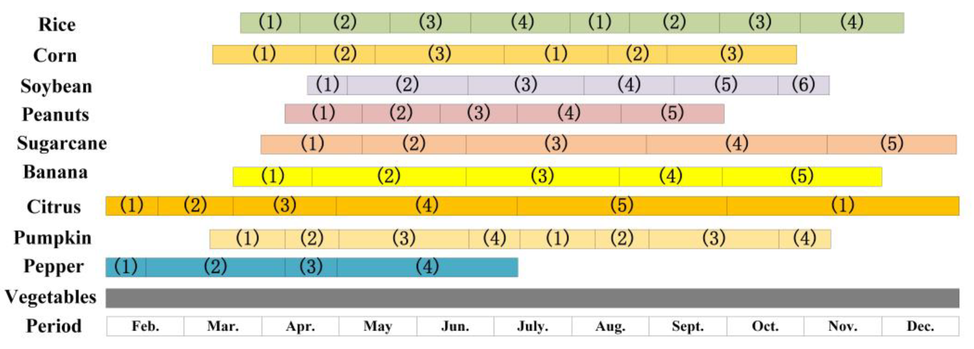
Drones 07 00285 g001
Figure 2. Crop growth stages in the study area. Rice: (1) seedling, (2) tillering, (3) spikelet development, (4) flowering and fruiting. Corn: (1) seedling, (2) spike, (3) flowering to maturity. Soybean: (1) emergence, (2) seedling, (3) flower bud differentiation, (4) blooming and fruiting, (5) seed filling period, (6) harvesting. Peanuts: (1) sowing and emergence, (2) seedling, (3) flowering needle, (4) pod, (5) package maturity. Sugarcane: (1) sowing to infancy, (2) emergence, (3) tillering, (4) elongation, (5) maturity. Banana: (1) seedling, (2) vigorous growth, (3) flower bud burst stage, (4) fruiting stages, (5) fruit development and harvest. Citrus: (1) flower bud differentiation, (2) budding, (3) flowering, (4) fruit growth and development, (5) fruit ripening, (6) flower bud differentiation. Pumpkin: (1) emergence, (2) rambling, (3) flowering, (4) harvesting. Pepper: (1) germination, (2) seedling, (3) flowering and fruit setting, (4) fruiting. Vegetables: vary from 60 to 120 days and grow all year round.
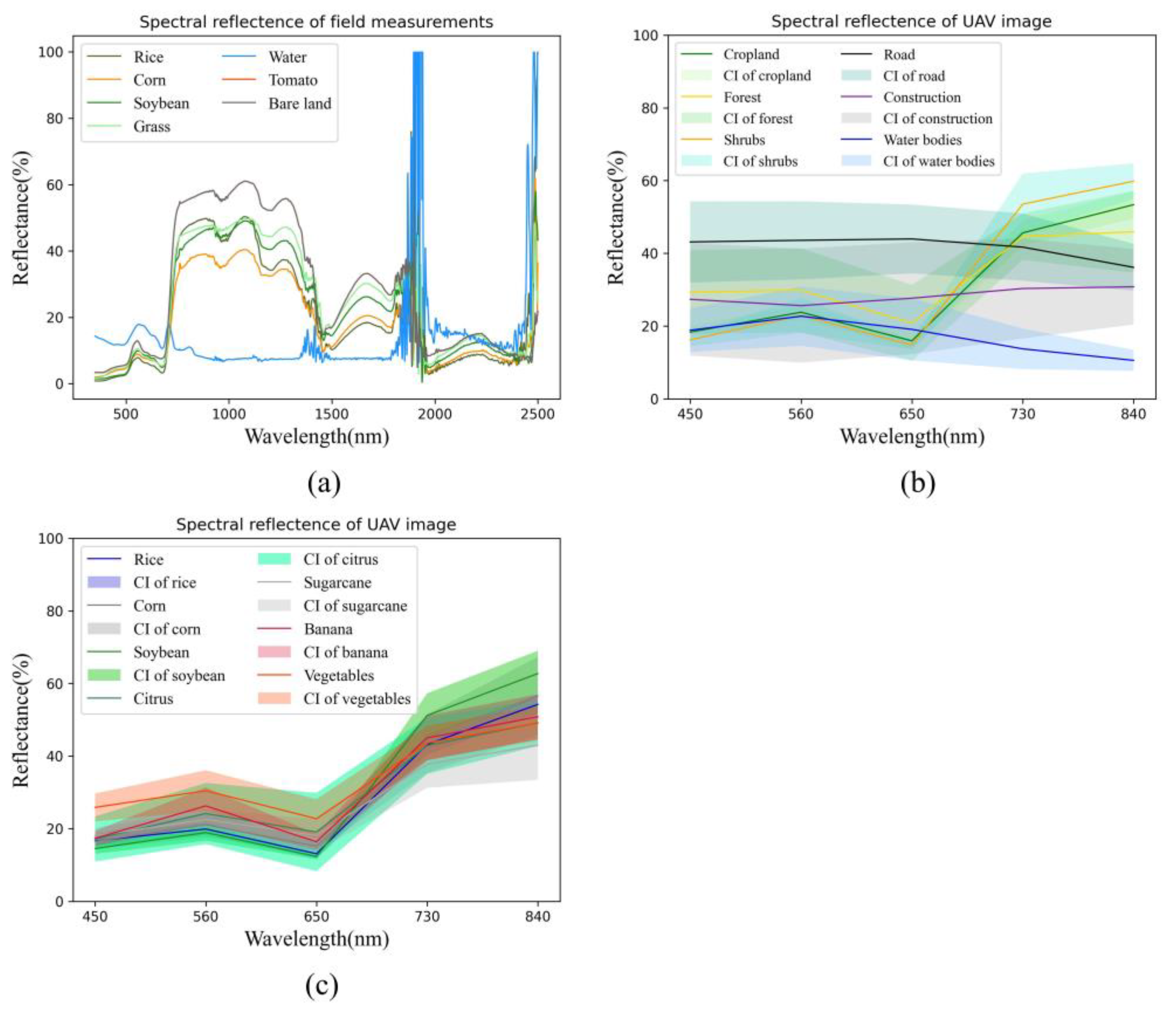
Drones 07 00285 g002
Figure 3. Spectral features of data from UAV and field measurements. Among them, spectral reflectance curves of some main crops in cropland parcels investigated through a spectroradiometer (a), and spectral reflectance curves and the confidence interval (CI) of main land classes and some main crops in the cropland parcels investigated through the UAV images (b,c).
Drones 07 00285 g003
Figure 4. U-Net (a) and U-Net++ (b) architecture.
Drones 07 00285 g004
Figure 5. Overall experiment framework.
Drones 07 00285 g005
Figure 6. The maps extracted from the test dataset of different (Convolutional neural network) CNN architectures are shown. (a) Original multispectral data (standard false color composited), (b) ground truth label, and (ch) results of experiments A1–A6.
Drones 07 00285 g006
Figure 7. The maps extracted from the test dataset of different spatial resolutions in experiment group B are shown. (a) Original multispectral data (standard false color composited), (b) ground truth label, and (cj) results of experiments B1–B8.
Drones 07 00285 g007
Figure 8. Local prediction details of the maps extracted from the test dataset in experiment group B are shown. (a-1) Original multispectral data (standard false color composited), (b-1) Ground truth, (c-1) the result of experiment B3, and (d-1) the result of experiment B6. (a-2,a-3) The local details of (a-1), corresponding to the black boxes of ground truth, (b-2,b-3) the local details in the black boxes of (b-1), (c-2,c-3) the local details in the black boxes of (c-1), and (d-2,d-3) the local details in the black boxes of (d-1).
Drones 07 00285 g008
Figure 9. The maps extracted from the test dataset of different spectral compositions in experiment group C are shown. (a) Original multispectral data (standard false color composited), (b) ground truth label, and (cf) results of experiments C1–C4.
Drones 07 00285 g009
Figure 10. Local prediction details of the maps extracted from the test dataset in experiment group C are shown. (a-1) Original multispectral data (standard false color composited), (b-1) ground truth, (c-1) the result of experiment C1, and (d-1) the result of experiment C4. (a-2,a-3) The local details of (a-1), corresponding to the black boxes of ground truth, (b-2,b-3) the local details in the black boxes of (b-1), (c-2,c-3) the local details in the black boxes of (c-1), and (d-2,d-3) the local details in the black boxes of (d-1).
Drones 07 00285 g010
Figure 11. The maps extracted from the test dataset of different terrain information in experiment group D are shown. (a) Original multispectral data (standard false color composited), (b) ground truth label, and (ce) results of experiments D1–D3.
Drones 07 00285 g011
Figure 12. Local prediction details of the maps extracted from the test dataset in experiment group D are shown. (a-1) Original multispectral data (standard false color composited), (b-1) ground truth, (c-1) the result of experiment D1, (d-1) the result of experiment D2, and (e-1) the result of experiment D3. (a-2a-4) The local details of (a-1), corresponding to the black boxes of ground truth, (b-2b-4) the local details in the black boxes of (b-1), (c-2c-4) the local details in the black boxes of (c-1), (d-2d-4) the local details in the black boxes of (d-1), and (e-2e-4) the local details in the black boxes of (e-1).
Drones 07 00285 g012
Figure 13. The maps extracted from more periods for the robustness test. (a) Ground truth label, (bd) original multispectral data (standard false color composited) collected from August, November, and December, respectively, and (eg) the maps extracted from August, November, and December, respectively.
Drones 07 00285 g013
Table 1. Related parameters of model training, among which: ‘learn rate decay = 0.9’: decaying the learn rate to 90% when it is needed, ‘time-validation = 3’: making a prediction on the validation dataset after every 3 training epochs, ‘patuence = 2’: decaying the learn rate if the effect of the model did not improve after 2 predictions on the validation dataset, and ‘epsilon = 0.001’: when the difference between the prediction loss function of the last two tests on the validation dataset is less than 0.001, it is considered that the model cannot be improved under the current learning rate, and the learning rate reduction mechanism needs to be triggered.
ItemParameter
Batch size12
OptimizerAdam
Maximum epochs350
Original learn rate1 × 10−4
Learn rate decay0.9
Minimum learn rate1 × 10−7
Time-validation3
Patuence2
Epsilon1 × 10−3
Table 2. Exploration of different down-sampling architectures of networks.
Experiment CodeNetworkSize of Max PoolingNumber of Down-Sampling Layers
A1U-Net(2,2)4
A2U-Net(2,2)5
A3U-Net(2,2)6
A4U-Net(4,4)3
A5U-Net++(2,2)4
A6U-Net++(4,4)3
Table 3. Exploration of the spatial resolution of different data.
Experiment CodeNetworkSpatial Resolution of Image (meters)
B1U-Net++0.3
B2U-Net++0.4
B3U-Net++0.5
B4U-Net++0.6
B5U-Net++0.7
B6U-Net++0.8
B7U-Net++0.9
B8U-Net++1.0
Table 4. Exploration of different spectral compositions of data.
Experiment CodeNetworkBands Composition of Image
C1U-Net++RGB
C2U-Net++RGB + RE
C3U-Net++RGB + NIR
C4U-Net++RGB + RE + NIR
Table 5. Exploration of different spectral compositions of data.
Experiment CodeNetworkBands’ Composition of Image
D1U-Net++RGB + RE + NIR + DSM
D2U-Net++RGB + RE + NIR
D3U-Net++RGB + RE + NIR + Slope
Table 6. Test (Overall accuracy) OA, Kappa coefficient, and (Intersection-over-Union) IoU of different network architectures.
A1A2A3A4A5A6
OA (%)83.589.988.286.091.390.4
Kappa (%)62.974.668.664.478.776.6
IoU (%)83.189.687.985.891.190.2
Table 7. Test OA, Kappa coefficient, and IoU of different network architectures.
B1B2B3B4B5B6B7B8
OA (%)94.294.194.593.993.893.992.792.3
Kappa (%)85.184.985.684.184.784.382.280.6
IoU (%)94.093.994.493.693.593.792.491.9
Table 8. Test OA, Kappa coefficient, and IoU of different network architectures.
C1C2C3C4
OA (%)94.592.594.095.6
Kappa (%)84.881.084.788.6
IoU (%)94.392.193.895.5
Table 9. Test OA, Kappa coefficient, and IoU of different network architectures.
D1D2D3
OA (%)95.694.595.9
Kappa (%)88.685.689.2
IoU (%)95.594.495.7
Table 10. Test OA, Kappa coefficient, and IoU of other periods.
AugustNovemberDecember
OA (%)97.296.996.5
Kappa (%)90.689.688.4
IoU (%)97.196.796.4
Disclaimer/Publisher’s Note: The statements, opinions and data contained in all publications are solely those of the individual author(s) and contributor(s) and not of MDPI and/or the editor(s). MDPI and/or the editor(s) disclaim responsibility for any injury to people or property resulting from any ideas, methods, instructions or products referred to in the content.

