Author Contributions
Conceptualization, B.B., B.T. and O.M.; methodology, O.M., B.P., A.B. and K.R.; software, K.R. and B.P.; formal analysis, M.V. and A.B.; investigation, B.I. and M.V.; resources, B.I. and M.V.; data curation, K.R. and B.I.; writing—original draft preparation, K.R.; writing—review and editing, B.B., O.M., B.I. and B.P.; supervision, O.M. and V.C.; project administration, B.B., V.C. and A.B.; funding acquisition, B.T., B.B. and V.C. All authors have read and agreed to the published version of the manuscript.
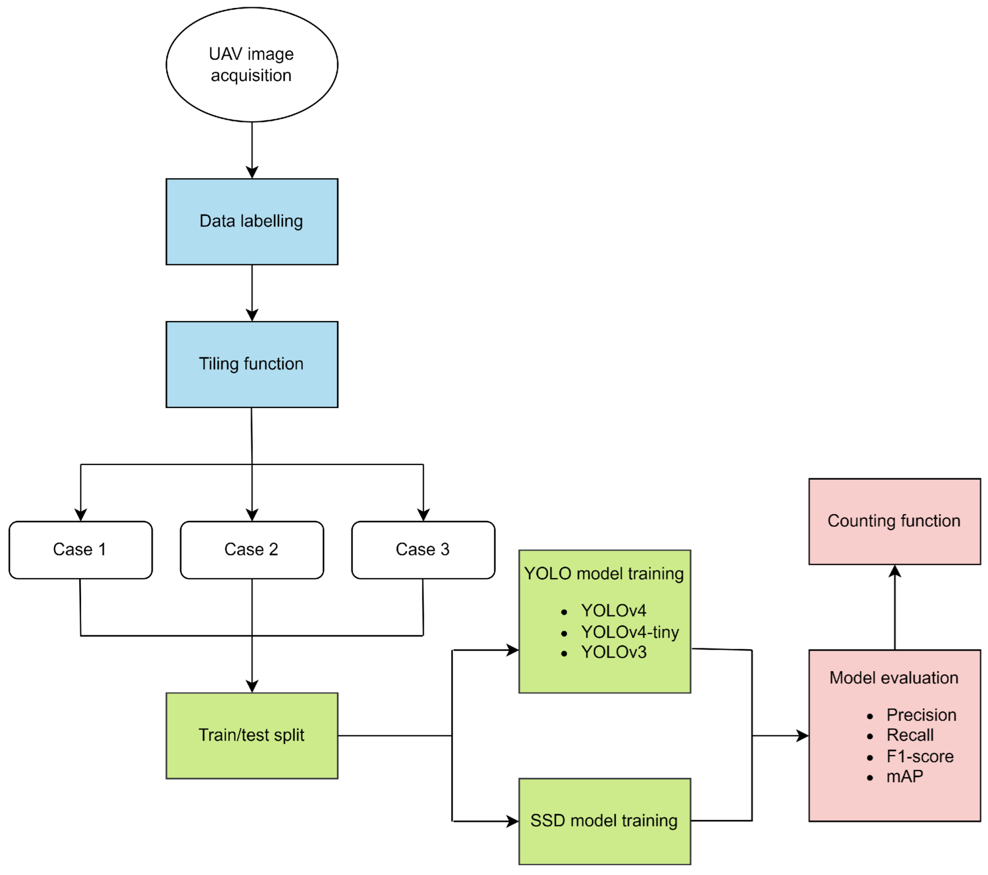
Figure 1.
Methodology flowchart of this study. Blue parts represent data preprocessing, green parts concern AI (artificial intelligence) model training, and red parts indicate the evaluation of the results using four metrics and a counting function.
Figure 1.
Methodology flowchart of this study. Blue parts represent data preprocessing, green parts concern AI (artificial intelligence) model training, and red parts indicate the evaluation of the results using four metrics and a counting function.
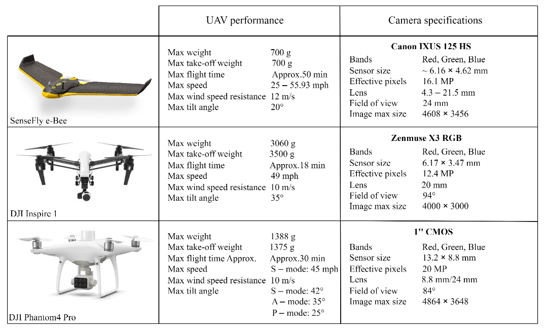
Figure 2.
UAV performances and camera specifications of platforms used for data acquisitions.
Figure 2.
UAV performances and camera specifications of platforms used for data acquisitions.
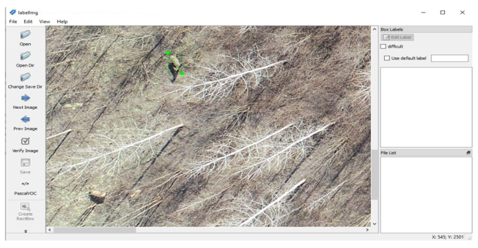
Figure 3.
Labeling with LabelImg tool.
Figure 3.
Labeling with LabelImg tool.
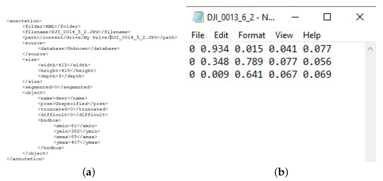
Figure 4.
Annotations generated by LabelImg tool. (a) Annotation in Pascal VOC format. (b) Annotation in YOLO format.
Figure 4.
Annotations generated by LabelImg tool. (a) Annotation in Pascal VOC format. (b) Annotation in YOLO format.
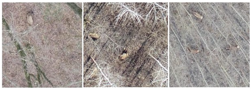
Figure 5.
Examples of positive samples, i.e., tiles containing at least one deer.
Figure 5.
Examples of positive samples, i.e., tiles containing at least one deer.
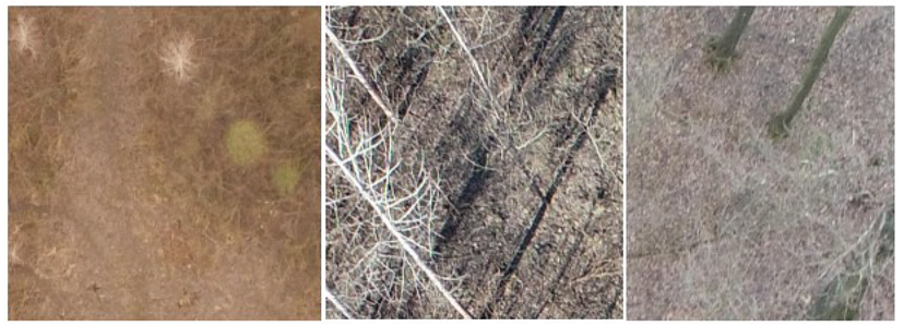
Figure 6.
Examples of negative samples, i.e., tiles without deer.
Figure 6.
Examples of negative samples, i.e., tiles without deer.
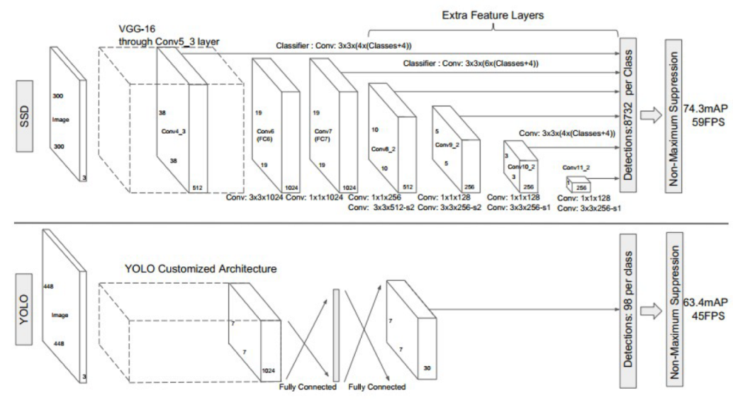
Figure 7.
A comparison between the SSD and YOLO network architectures [
21]. The architecture of YOLO uses an intermediate fully connected layer instead of the convolutional filter used in SSD for the final predictions.
Figure 7.
A comparison between the SSD and YOLO network architectures [
21]. The architecture of YOLO uses an intermediate fully connected layer instead of the convolutional filter used in SSD for the final predictions.
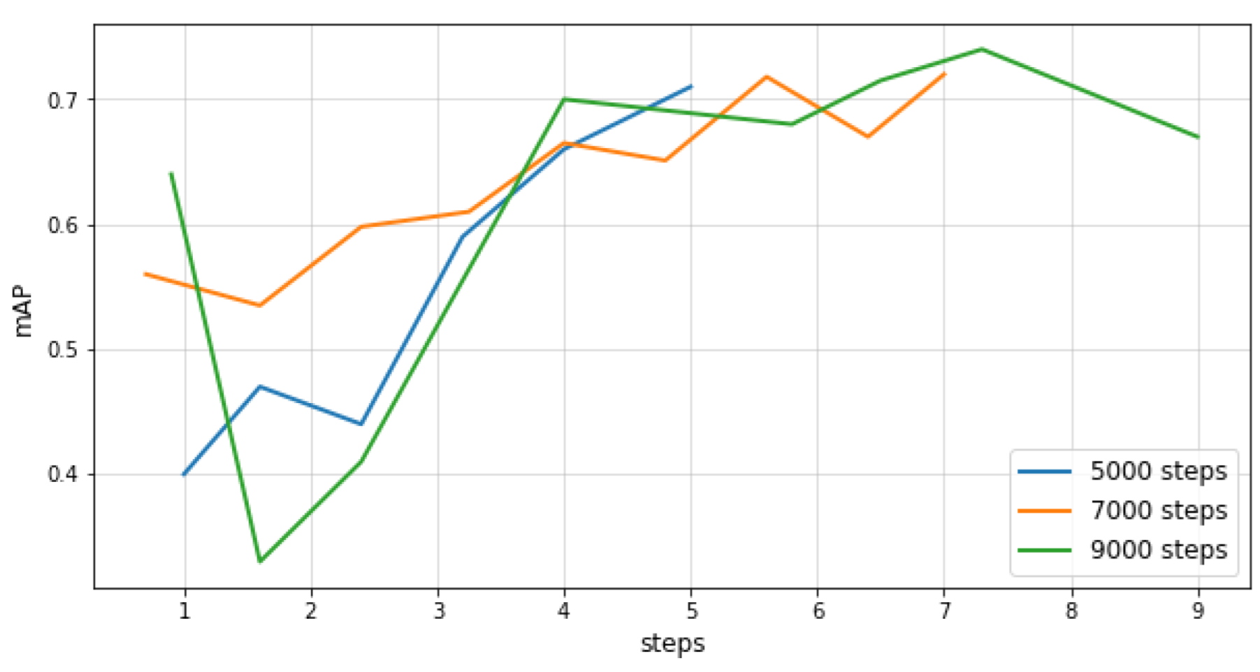
Figure 8.
mAP@.50 IOU curves for different numbers of training steps for the Single Shot Detector.
Figure 8.
mAP@.50 IOU curves for different numbers of training steps for the Single Shot Detector.
Figure 9.
mAP@.75 IOU curves for different numbers of training steps for the Single Shot Detector.
Figure 9.
mAP@.75 IOU curves for different numbers of training steps for the Single Shot Detector.
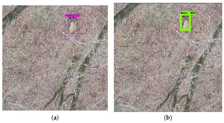
Figure 10.
Confidence score of YOLOv4 (a) and SSD (b) on the same image. (a) You Only Look Once version 4. (b) Single Shot Multibox Detector.
Figure 10.
Confidence score of YOLOv4 (a) and SSD (b) on the same image. (a) You Only Look Once version 4. (b) Single Shot Multibox Detector.
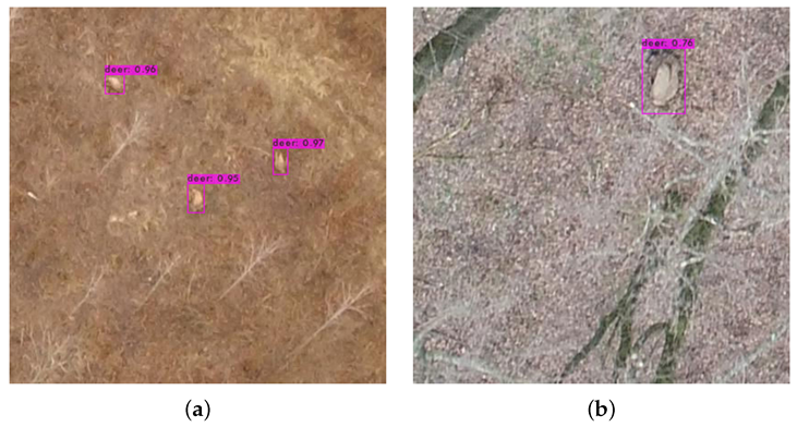
Figure 11.
Comparison of YOLOv4-tiny performance for detecting small (a) and medium objects (b).
Figure 11.
Comparison of YOLOv4-tiny performance for detecting small (a) and medium objects (b).
Figure 12.
mAP@.50 IOU—the average precision using IOU = 0.5 for the first case (left) and the third case (right).
Figure 12.
mAP@.50 IOU—the average precision using IOU = 0.5 for the first case (left) and the third case (right).
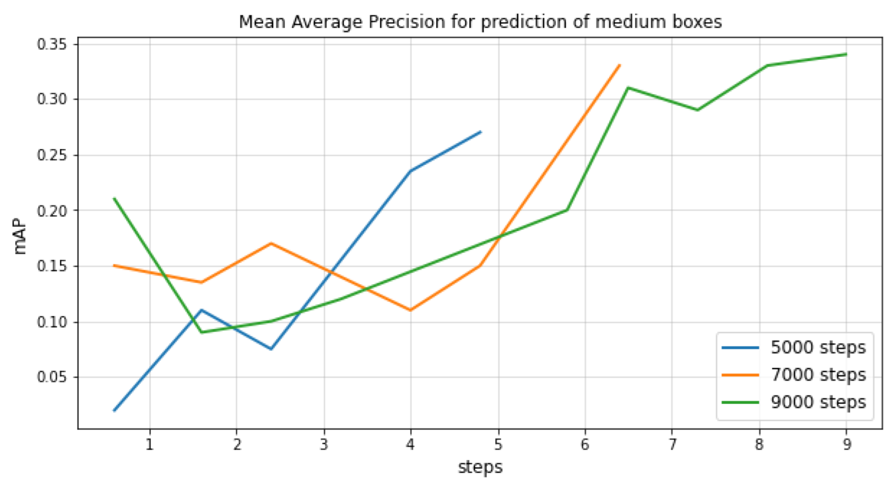
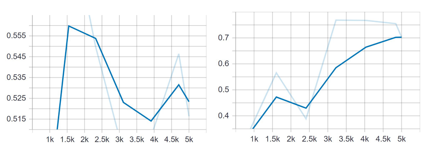
Figure 13.
Mean average precision for small and medium objects when trained on the set of 240 images, of which 120 were positive and 120 negative samples. (a) Detection of small objects. (b) Detection of medium objects.
Figure 13.
Mean average precision for small and medium objects when trained on the set of 240 images, of which 120 were positive and 120 negative samples. (a) Detection of small objects. (b) Detection of medium objects.
Figure 14.
Mean average recall for detecting small and medium bounding boxes from 240 images after 5000 steps of training. (a) Detection of small objects. (b) Detection of medium objects.
Figure 14.
Mean average recall for detecting small and medium bounding boxes from 240 images after 5000 steps of training. (a) Detection of small objects. (b) Detection of medium objects.
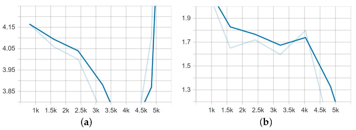
Figure 15.
Classification and localization loss of the SSD model trained on 1989 images for 5000 steps. (a) Classification loss. (b) Localization loss.
Figure 15.
Classification and localization loss of the SSD model trained on 1989 images for 5000 steps. (a) Classification loss. (b) Localization loss.
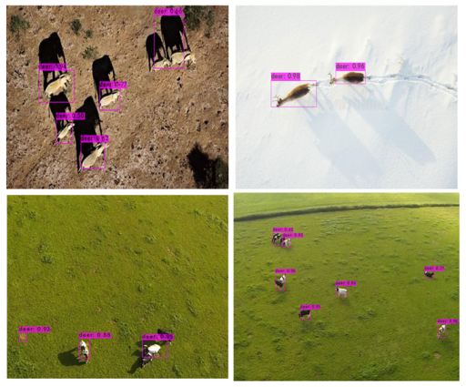
Figure 16.
Results of YOLOv4 when applied to new images with different backgrounds to those in the training set.
Figure 16.
Results of YOLOv4 when applied to new images with different backgrounds to those in the training set.
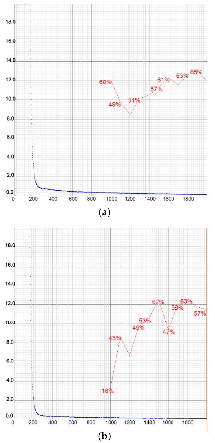
Figure 17.
Loss and mAP performance during the training of YOLOv4 in the first case.
Figure 17.
Loss and mAP performance during the training of YOLOv4 in the first case.
Figure 18.
Representations of loss and mAP values during the training of YOLOv3 in the first (a) and second (b) cases.
Figure 18.
Representations of loss and mAP values during the training of YOLOv3 in the first (a) and second (b) cases.
Figure 19.
Illustration of bounding boxes and confidence score predictions of YOLOv3 in the second case, when it achieved the highest mAP.
Figure 19.
Illustration of bounding boxes and confidence score predictions of YOLOv3 in the second case, when it achieved the highest mAP.
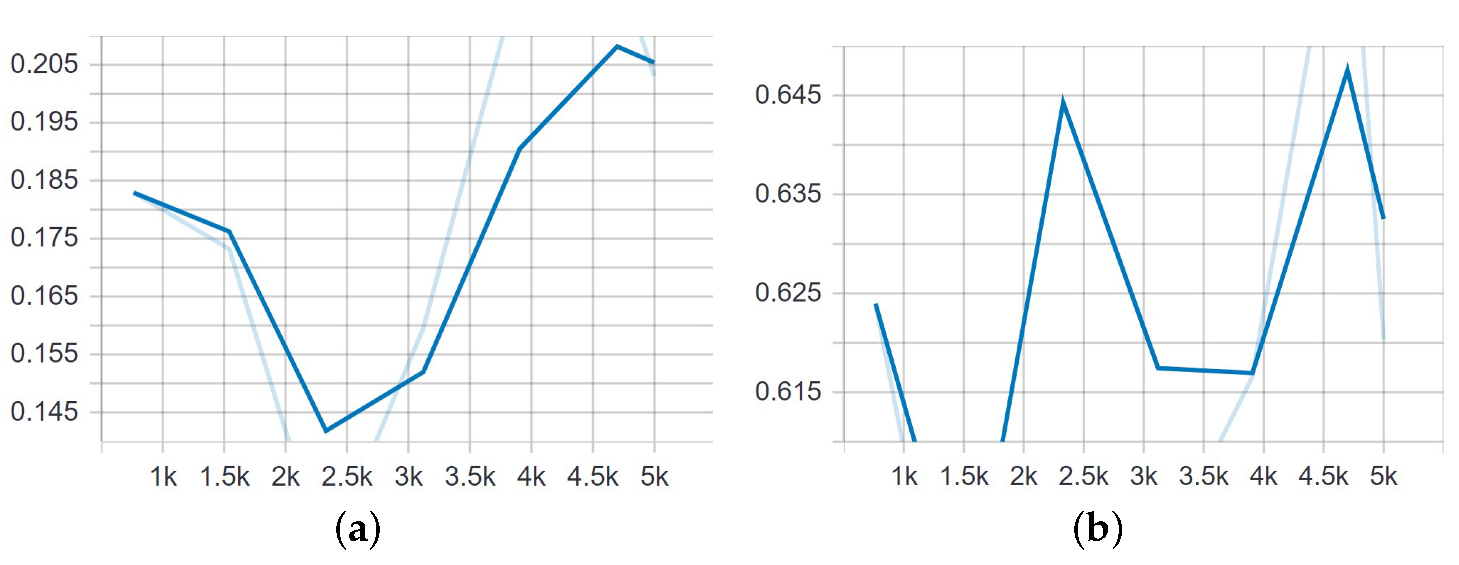
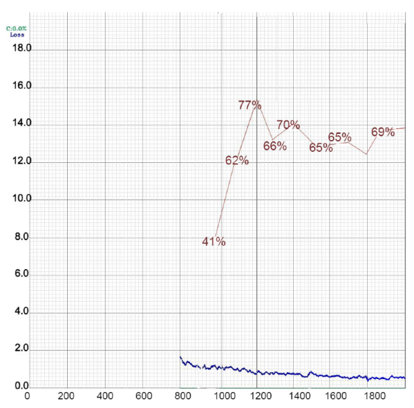
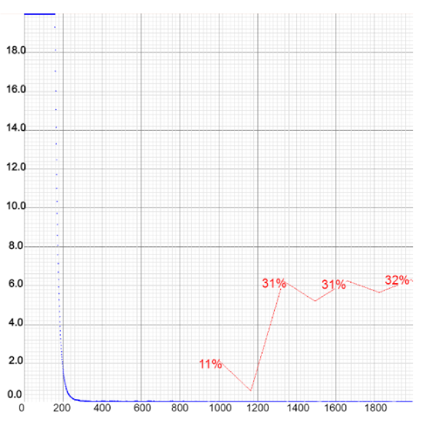
Figure 20.
Representations of loss and mAP values during the training of YOLOv4-tiny in the first two setups, with a different number of training images. In the first case (a), the highest mAP achieved was 65.11%, while in the second case (b) that value was slightly lower at 63.00%. The loss value remained low at all times. (a) Setup 1. (b) Setup 2.
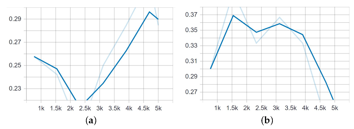
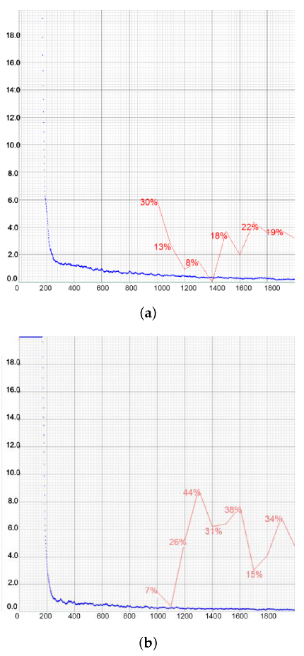
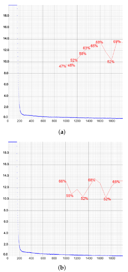
Figure 21.
Representations of loss and mAP values during the training of YOLOv4-tiny in the setup with the highest number of training images. Chart shows poor performance of the model due to the large number of negative samples. The loss value remained low.
Figure 21.
Representations of loss and mAP values during the training of YOLOv4-tiny in the setup with the highest number of training images. Chart shows poor performance of the model due to the large number of negative samples. The loss value remained low.
Figure 22.
Charts of the YOLOv4-tiny training with the network resolution increased to 512 × 512 (a) and 608 × 608 (b).
Figure 22.
Charts of the YOLOv4-tiny training with the network resolution increased to 512 × 512 (a) and 608 × 608 (b).
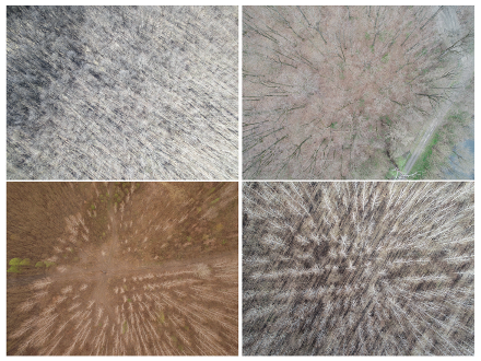
Figure 23.
Example of the image diversity of our dataset. There were huge variations in the background, with illumination differences due to weather, season, and shadows.
Figure 23.
Example of the image diversity of our dataset. There were huge variations in the background, with illumination differences due to weather, season, and shadows.
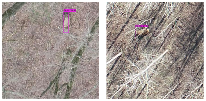
Figure 24.
Illustration of false negative predictions of YOLOv4 (left) and SSD (right) models. We can see that this could happen when the object appeared blurry (as in the left case) or when the animal was overlapped by branches or in motion (as in the right case).
Figure 24.
Illustration of false negative predictions of YOLOv4 (left) and SSD (right) models. We can see that this could happen when the object appeared blurry (as in the left case) or when the animal was overlapped by branches or in motion (as in the right case).
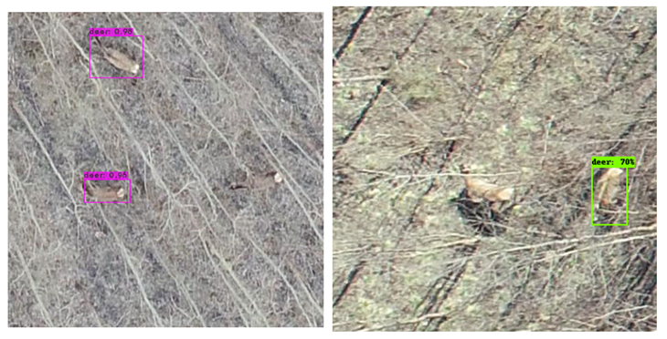
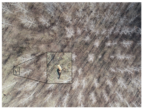
Figure 25.
Example of small target objects in our input images. Given an image this large, it is difficult to locate and recognize the animal, for both humans and machines.
Figure 25.
Example of small target objects in our input images. Given an image this large, it is difficult to locate and recognize the animal, for both humans and machines.
Table 1.
Details of the images provided and the number of labels.
Table 1.
Details of the images provided and the number of labels.
| | No. of Images | No. of Deer Recorded |
|---|
| 4608 × 3456 | 2 | 2 |
| 4864 × 3648 | 16 | 87 |
| 4000 × 3000 | 12 | 80 |
| Total | 30 | 169 |
Table 2.
Configuration of hyperparameters of each model.
Table 2.
Configuration of hyperparameters of each model.
| | YOLOv4 | YOLOv4-tiny | YOLOv3 | SSD |
|---|
| Batch size | 64 | 64 | 10 | 24 |
| Momentum | 0.949 | 0.9 | 0.9 | 0.9 |
| Learning rate | 0.001 | 0.00261 | 0.001 | 0.004 |
| Decay | 0.0005 | 0.0005 | 0.0005 | 0 |
Table 3.
Object detection methods used and their performance metrics.
Table 3.
Object detection methods used and their performance metrics.
| Method | Benchmark Dataset | Metrics |
|---|
| SSD | COCO | mAP; mAP@.50; mAP@.75; APS; APM; APL;
AR1; AR10; AR100; ARS; ARM; ARL |
| YOLOv3 | COCO | mAP; mAP@.50; mAP@.75; APS; APM; APL;
AR1; AR10; AR100; ARS; ARM; ARL |
| YOLOv4 | COCO | mAP; mAP@.50; mAP@.75; APS; APM; APL |
Table 4.
Comparison of the best results achieved by each model and the case in which they were achieved.
Table 4.
Comparison of the best results achieved by each model and the case in which they were achieved.
| Model | mAP | Recall | Case |
|---|
| YOLOv4 | 0.71 | 0.75 | 2nd |
| SSD | 0.70 | 0.39 | 3rd |
| YOLOv4-tiny | 0.65 | 0.62 | 1st |
| YOLOv3 | 0.38 | 0.25 | 2nd |
Table 5.
Results achieved by all the models in the first case.
Table 5.
Results achieved by all the models in the first case.
| | Precision | Recall | F1 Score | mAP |
|---|
| YOLOv4 | 0.83 | 0.62 | 0.62 | 0.69 |
| YOLOv4-tiny | 0.79 | 0.62 | 0.70 | 0.65 |
| YOLOv3 | 0.70 | 0.30 | 0.42 | 0.30 |
Table 6.
Results achieved by all the models in the second case.
Table 6.
Results achieved by all the models in the second case.
| | Precision | Recall | F1 Score | mAP |
|---|
| YOLOv4 | 0.86 | 0.75 | 0.80 | 0.71 |
| YOLOv4-tiny | 0.83 | 0.42 | 0.56 | 0.63 |
| YOLOv3 | 0.75 | 0.25 | 0.38 | 0.38 |
Table 7.
Results achieved by all the models in the third case.
Table 7.
Results achieved by all the models in the third case.
| | Precision | Recall | F1 Score | mAP |
|---|
| YOLOv4 | 0.60 | 0.46 | 0.52 | 0.51 |
| YOLOv4-tiny | 0.40 | 0.31 | 0.35 | 0.32 |
| YOLOv3 | 0 | 0 | 0 | 0.18 |


 ,
, 


