Article

Two-Step Approach toward Alignment of Spatiotemporal Wide-Area Unmanned Aerial Vehicle Imageries

1
Department of Computer Science and Artificial Intelligence, Jeonbuk National University, Jeonju 54896, Republic of Korea
2
Department of Mechatronics Engineering, Jeonbuk National University, Jeonju 54896, Republic of Korea
3
LANL-JBNU Engineering Institute-Korea, Jeonbuk National University, Jeonju 54896, Republic of Korea
4
Spatial Information Research Institute, Korea Land and Geospatial Informatix Corporation, Jeonju 54870, Republic of Korea
5
Department of Flexible and Printable Electronics, Jeonbuk National University, Jeonju 54896, Republic of Korea
6
Center for Advanced Image Information Technology, Jeonbuk National University, Jeonju 54896, Republic of Korea
*
Author to whom correspondence should be addressed.
Drones 2023, 7(2), 131; https://doi.org/10.3390/drones7020131
Submission received: 27 December 2022 / Revised: 7 February 2023 / Accepted: 9 February 2023 / Published: 12 February 2023

Abstract

:
Recently, analysis and decision-making based on spatiotemporal unmanned aerial vehicle (UAV) high-resolution imagery are gaining significant attention in smart agriculture. Constructing a spatiotemporal dataset requires multiple UAV image mosaics taken at different times. Because the weather or a UAV flight trajectory is subject to change when the images are taken, the mosaics are typically unaligned. This paper proposes a two-step approach, composed of global and local alignments, for spatiotemporal alignment of two wide-area UAV mosaics of high resolution. The first step, global alignment, finds a projection matrix that initially maps keypoints in the source mosaic onto matched counterparts in the target mosaic. The next step, local alignment, refines the result of the global alignment. The proposed method splits input mosaics into patches and applies individual transformations to each patch to enhance the remaining local misalignments at patch level. Such independent local alignments may result in new artifacts at patch boundaries. The proposed method uses a simple yet effective technique to suppress those artifacts without harming the benefit of the local alignment. Extensive experiments validate the proposed method by using several datasets for highland fields and plains in South Korea. Compared with a recent work, the proposed method improves the accuracy of alignment by up to 13.21% over the datasets.

1. Introduction

Recent progress in the growth monitoring of crops through unmanned aerial vehicles (UAVs) has enabled a wide variety of applications for precision farming, including crop yield and disease management [1,2,3]. UAVs have significant advantages in terms of easy control, which helps in capturing narrow areas as high-resolution aerial images (approximately 0.1 m) from low-altitude flights (e.g., 30–60 m) [4,5,6]. Airplanes or satellites can contain the entire target site in a single shot. Thus, scanning a whole target site typically results in multiple UAV images that are used to create a single wide-area image mosaic for further analysis, such as estimation of the vegetation index [7], crop yield [8,9], and monitoring environment [10,11].
Besides the use of a single image, time-series monitoring and analysis are gaining research attraction in various domains of data-driven smart agriculture, such as growth monitoring, yield estimation, and climate forecasting. Early approaches to corn yield prediction proposed multilayer perceptron neural networks that use environmental data of genotype and climate [12]. A decision tree is widely used to detect changes in field usage from multispectral satellite orthography [13] or classify between wetland and dryland from images with a resolution of 5 m [14]. Recently, advanced neural networks have been used, which include long short-term memory (LSTM) with climate data [15], recurrent convolutional neural network (CNN) with previous yield, climate, and soil data [16], and transfer learning for the prediction of soybean and corn yield [16]. The approach proposed in [17] used convolutional LSTM with radar data of satellites for weather forecasting. In [18], a CNN-based method has been proposed to perform crop classification from temporal multispectral satellite images of low resolutions (4–8 m) [19]. Temporal satellite images are also used for managing crop disease by monitoring its growth status [20]. A LiDAR sensor is used to constitute temporal data with satellite orthography for crop classification [21] or, with the temporal vegetation index, to classify the severity level of forest fires [22].
Spatiotemporal data in those approaches typically consisted of spatially aligned orthoimages taken hours to years apart. An orthoimage is an aerial image geometrically corrected, i.e., orthorectified, such that its scale is uniform, accurately representing the Earth’s surface. An orthophotomosaic is a raster image made by merging orthoimages. Conventionally, orthoimages are generated by using dense point cloud or digital models (DMs) such as the digital building model (DBM), the digital terrain model (DTM) [23], and the digital surface model (DSM) [24], to detect overlapped regions and recover the occluded area. Recent advances in orthoimage generation based on deep neural networks (DNNs) include resolution improvement of the digital elevation model (DEM) [25], generation of DEM from a single image [26], and detection of the occluded area through a point cloud model [27]. These approaches require precise exterior orientation parameters by using trilateration or a 3D model of high resolutions, thus being computationally expensive.
In addition, most existing approaches rely on spatiotemporal low-resolution satellite images obtained at distances of several meters [14,18,19] to even kilometers [16]. Their spatial alignment is relatively straightforward but results in limited applications. On the other hand, UAV imagery of high-resolutions allows us to analyze and monitor crop growth more finely. For example, it is possible to precisely manage wheat diseases from UAV images of high resolution, e.g., 3.4 cm/px [28]. Its applications include crop classification and identification [29], crop yield prediction [2,30], crop height estimation from 3D point clouds [31], health monitoring of roots [32], and estimating surface fluxes from a vegetation index [33]. Spatially aligning high-resolution images, however, requires mosaicking multiple UAV images into a large one, which is challenging compared with low-resolution counterparts.
Image mosaicking typically is comprised of three steps: image registration, seam cutting, and image blending. Image registration extracts overlapped areas to find a homography for geometrically matching adjacent images. Although this stage requires global positioning system (GPS) data or georeferenced information, the absence of this information, which is prevalent, can be resolved by keypoint-extraction methods, such as phase correlation [34], SIFT [35] and spatial transformation [36,37]. Seam cutting aims to find a joining boundary that is natural and visually indistinguishable without artifacts [38,39]. Image blending is the last step to refine the seam boundary in an image mosaic [40]. Although recent DNN-based approaches have enhanced the performance of each step, for instance, image registration [41,42,43,44,45], and seam cutting [46,47], they are not suitable for wide-area images of high resolutions. In contrast, conventional alignment algorithms are able to handle images with arbitrary resolutions.
UAV operations are usually affected by time-variant factors, such as weather conditions. Therefore, image acquisitions over a whole target site are highly likely inconsistent, necessitating individual transformations locally to subregions or patches of the mosaics. However, recent image-alignment methods are primarily applicable for images with relatively small resolutions [41,42,43,44,45,48]. Furthermore, the naive application of independent transformations to the patches of the mosaics may cause unexpected artifacts along patch boundaries.
To address these difficulties, this paper proposes a simple yet effective method by which to construct high-resolution spatiotemporal imagery from UAV images of a wide-area target site. Our method performs a geometrical alignment of a wide-area mosaic, called source, with its counterpart called target, which have been taken several days or weeks apart. The proposed approach consists of two steps: (1) global alignment, in which the keypoints coexisting in two image mosaics are matched through a single transformation matrix, called homography, and (2) local alignment, which refines misalignments by using per-patch transformations. Our approach combines a conventional keypoint-matching algorithm and a keypoint-extraction technique by using a DNN. A conventional keypoint matching [49] is applicable to images of arbitrary resolutions but with limited accuracy [35,36,37,49,50]. In contrast, DNN-based methods better predict the relevant transformation for keypoint matching, outperforming the conventional ones [41,42,43,44,45,48]. Although CNNs are popular for this purpose, the size of input images is restricted, usually as patches with resolutions of millions of pixels, due to the internal structure of CNNs [48]. The image alignment is based on keypoints that appear robustly and repetitively in images. Identifying such keypoints is challenging for farmland photos wherein patterns of color and texture are often largely repetitive. For this purpose, the proposed method adopts a DNN-based method to extract trustworthy keypoints.

2. Materials and Methods

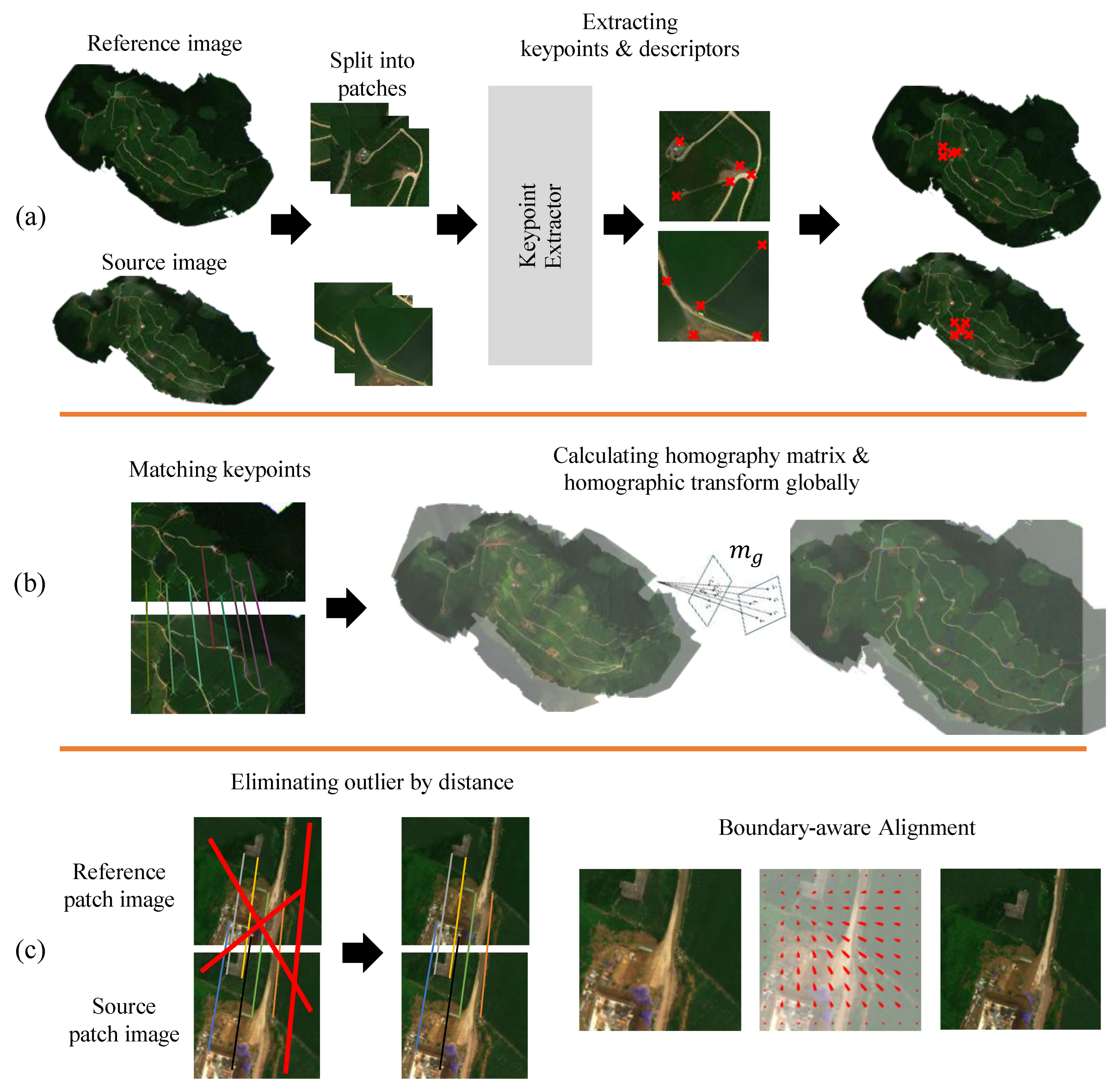
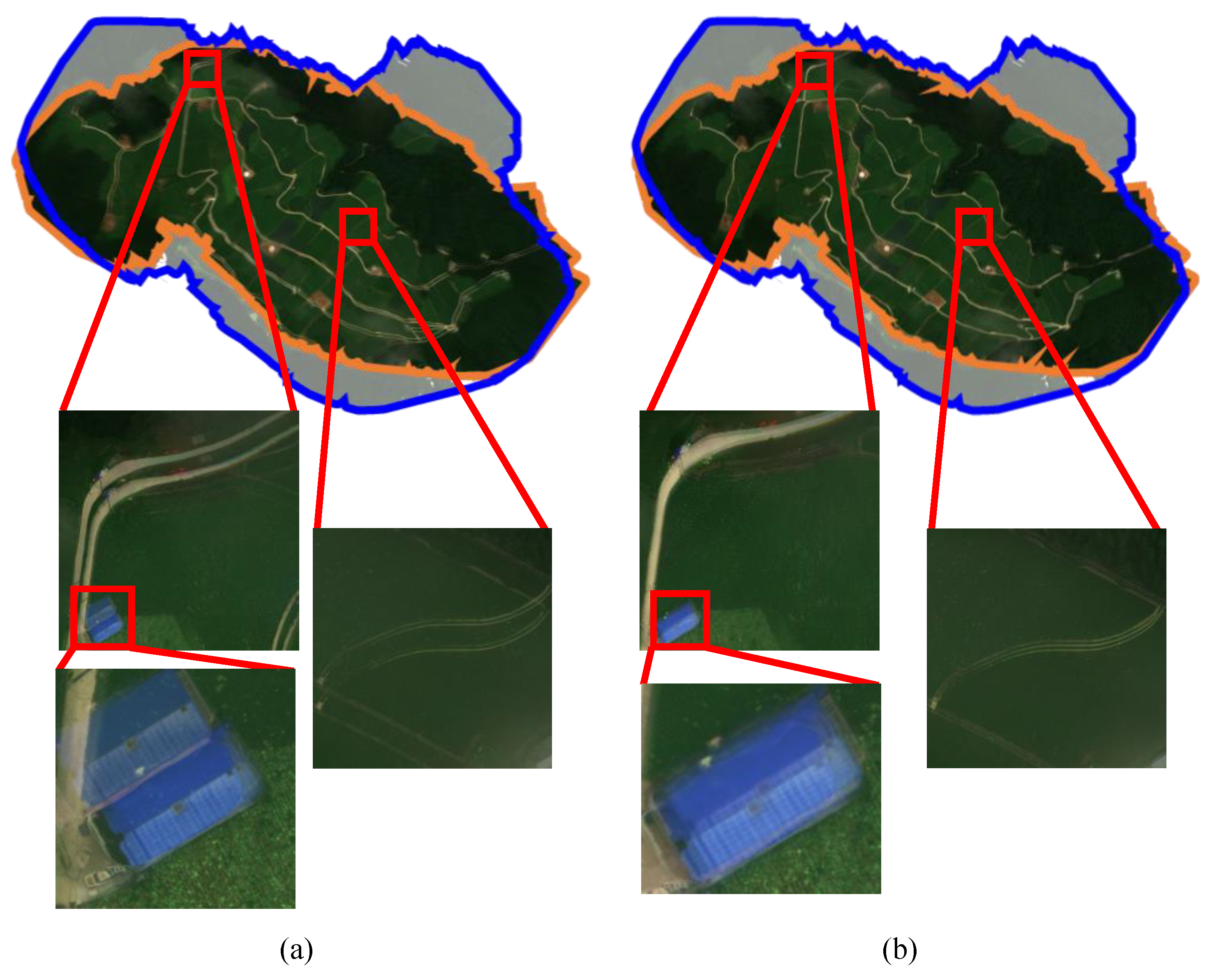
2.1. Problem Definition and Method Overview

Problem Definition. Let X s and X t be two input images, namely source and target, respectively. We assume that each input image is a wide-area mosaic of high resolutions built from UAV images with an identical time tag (usually the same date) for a study site. The mosaic images are created independently with different time tags and are spatially misaligned. The source and target have an equal number of multispectral bands, including the conventional RGB channels. For simplicity, we assume images of a single channel represented as 2D (width and height) without loss of generality.
We also assume that the input mosaics are annotated with reference points, which are pixels corresponding to reliably different locations over the input images. Time-invariant structures or geographical patterns are well suited to being reference points. Typical examples of reference points include predefined GCPs and corners of buildings and roads of unique curvature. Let R s and R t be sets of 2D pixel coordinates for reference points in X s and X t , respectively, and R s = R t . Then, our objective is to find a set of transformations to align the source X s with the target X t in a way that the distance between the corresponding reference points R t and R s is minimized:
m g , M l = arg min m g * , M l * d R t , T m g * , M l * , R s ,
where m g is a global mapping (or transformation) that maps the coordinates in R s to their counterparts in R t (Section 2.2), and M l is a set of local mappings applied to each patch of X s respectively (Section 2.3). T ( · ) is a set of reference points in the source (i.e., R s ) that are transformed through the global and local alignments, m g and M l . d ( · ) is a distance measure between two point sets (Section 3.4). Table 1 provides a summary of notations used throughout the paper.
Method Overview. We first perform the global alignment of X s with respect to X t as shown in Figure 1b. At the outset, the keypoints in X s and X t were extracted and matched. This step aims to find a mapping that best aligns keypoints in X s with their counterparts in X t . We adopted a DNN-based method to extract keypoints and their descriptors [42]. Note that any keypoint extractor can be used in this step. Reference points, R s and R t , and keypoints are conceptually similar in that they represent time-invariant and unique locations of the target site. However, there are two essential differences between them. First, we use the reference points to evaluate the alignment accuracy only at the end, whereas keypoints were intermediate data for finding mappings m g and M l in Equation (1). Secondly, not all keypoints are meaningful; thus, outliers in matched keypoint pairs may exist.
We use homography as a mapping m g in the global alignment. For this purpose, we adopted an algorithm to align the keypoint pairs, known as the random sample consensus (RANSAC) [49], owing to its applicability in aligning high-resolution images and robustness for outlier keypoint pairs. RANSAC is an iterative method that estimates the parameters of a mathematical model for a given set of observations, i.e., keypoint pairs, allowing outliers if they do not affect the values of the estimates. The detailed description of RANSAC is beyond the scope of this paper. The global alignment provides an initial alignment of the source with the target, as shown in Figure 2. The figure also shows that the alignment is incomplete yet. Then, the local alignment splits each input image into small patches from the global alignment and finds individual local mappings well-suited for the patches. However, the straightforward merge of those independently transformed patches into a single mosaic may result in artifacts at patch boundaries, as depicted in Figure 3.

2.2. Global Alignment

Review of Homographies. We first provide a brief review of the homography, which is represented as a matrix h R 3 × 3 :
h = h 11 h 12 h 13 h 21 h 22 h 23 h 31 h 32 1 .
Homography h maps (or projects) pixel ( x , y ) in the source image to pixel x , y in the target image as
h x y 1 T = h 11 x + h 12 y + h 13 h 21 x + h 22 y + h 23 h 31 x + h 32 y + 1 = u v w = w x w y w ,
where w R is a scaling factor of the x- and y-axes with respect to the z-axis by the projection. For example, if homographies are
h s = h 11 0 0 0 h 22 0 0 0 1 , h t = 1 0 h 13 0 1 h 23 0 0 1 , and h r = cos θ sin θ 0 sin θ cos θ 0 0 0 1 ,
then h s scales an image in the x- and y-coordinates with corresponding scale factors h 11 and h 22 , h t translates the image by h 13 and h 23 along the x- and y-axes, respectively. Lastly, applying h r rotates the image counterclockwise by θ .
For given N keypoint pairs x i , y i , x i , y i i = 0 N , h is calculated by solving a linear system U h = 0 , where
U = x 1 y 1 1 0 0 0 x 1 x 1 x 1 y 1 x 1 0 0 0 x 1 y 1 1 y 1 x 1 y 1 y 1 y 1 x N y N 1 0 0 0 x N x N x N y N x N 0 0 0 x N y N 1 y N x N y N y N y N and h = h 11 h 12 h 13 h 21 h 22 h 23 h 31 h 32 1 T .
Although h ^ can be calculated with only four point pairs, typically we have more keypoint pairs, which leads us to define the least square problem as
h = arg min h * U h * 2 .
A solution to Equation (5) is the eigenvector of U T U with the smallest eigenvalue.
Keypoint Extraction. Keypoints for aligning two images should be reliable in that they can be distinguished from other pixels in an image. In addition, the location indicated by a keypoint pair should appear across images repetitively. Those keypoints are represented by descriptors that are usually multidimensional vectors [35,42,43,44,45]. If pixels in different images have similar descriptors, they are likely to be similar geographical locations. Let C s = c s , i be a set of keypoints for X s and φ c s , i be its multidimensional descriptor. Similarly, C t = c t , i corresponds to X t , where C t C s in general.
Calculating m g in Equation (1) requires a set of matched keypoints from C s and C t in terms of descriptors. Keypoints are selected from C s and reordered as C s = k i , such that k i is a keypoint of the source matched to keypoint c t , i of the target satisfies
φ c t , i φ k i φ c t , i φ c s , j k i , c s , j C s and k i c s , j .
As a result, the number of matched keypoints pairs is C s .
Determining Homography. Keypoint matching in Equation (6) may include outlier keypoint pairs because multiple keypoints in C s may be matched to the same keypoint in C t . For example, in agricultural UAV images, the proliferation of similar visual patterns appears at farm boundaries and roads, and therefore pretty distal keypoints with similar descriptors could be made. As discussed earlier, we use RANSAC to estimate m g from matched keypoints. For given mapping m g , we denote a transformed source image by X g = m g X s . In other words, for given pixels ( x , y ) X s and x , y X g , from Equation (3), it holds that
w x   y   1 T = m g · x   y   1 T .

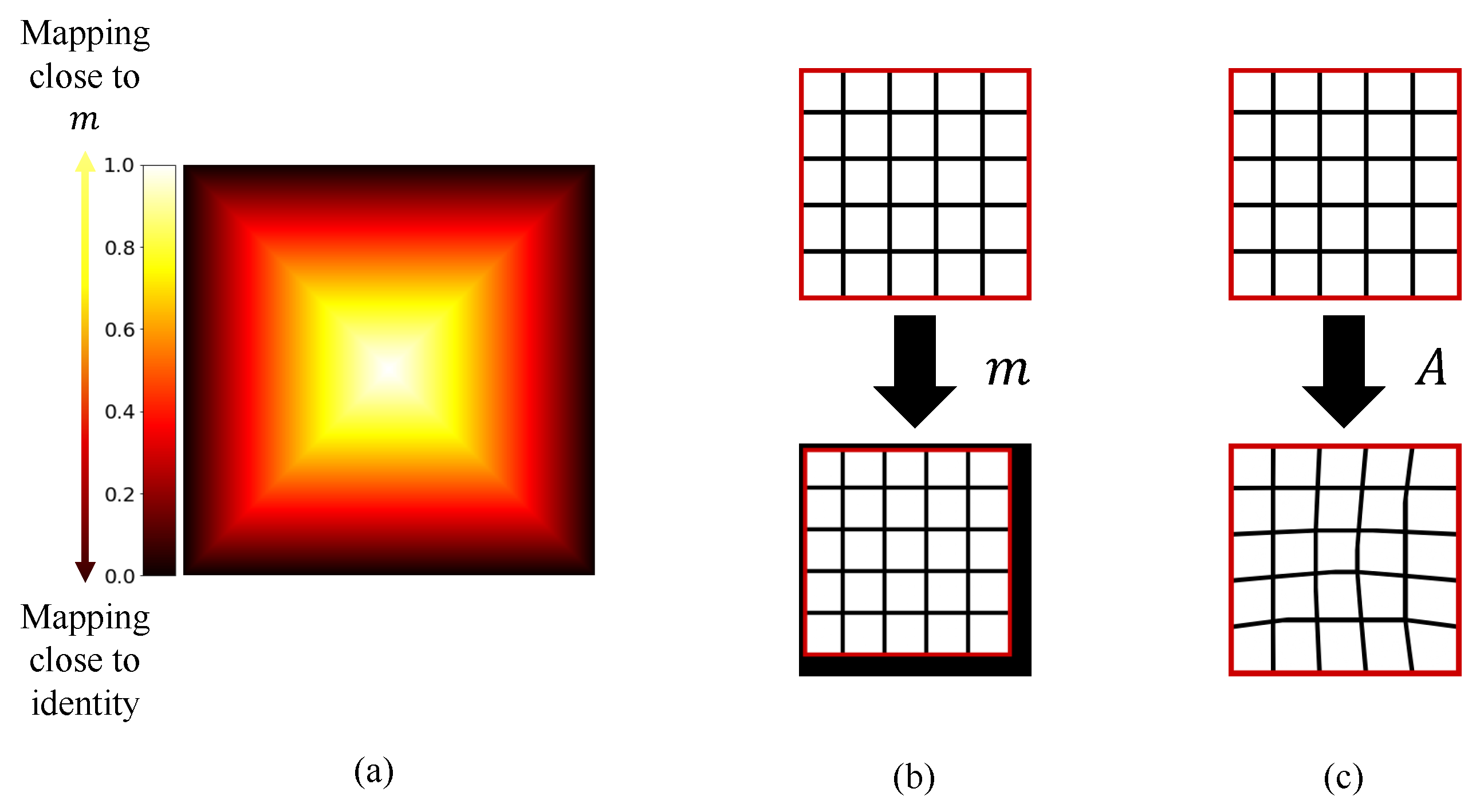
2.3. Local Alignment

Even though the global alignment provides a proper alignment of the source mosaic only with a single homography m g , local misalignments may persist, as shown in Figure 2. Let P g = p g ( i ) be a set of nonoverlapped patches for the transformed source image X g and P t = p t ( i ) be a set of patches for the target X t . Moreover, let K g be keypoints in X g , i.e., transformed keypoints of X s . Then, each local mapping m i l M l is estimated for corresponding patches of P g and P t . After the global alignment, patches of the inputs with the same index, for example, p g ( i ) X g and p t ( i ) X t , are likely to overlap with each other significantly. Therefore, it is natural to take m i l as a mapping concerning the patches. Furthermore, such spatial proximity information between p g ( i ) and p t ( i ) enables us to identify the fidelity of the keypoint pairs established in the global alignment step, wherein no distance information between the source and target was available. In particular, we use a threshold on the pixel distance of the matched keypoints to exclude outlier pairs before estimating patch-level homographies. As a result, we obtain refined keypoints for patch p g ( i ) , denoted by K g ( i ) K g , and p t ( i ) , by K t ( i ) C t for the local alignment. Then, distance between pixels in p g ( i ) and p t ( i ) is no larger than a threshold τ l , which is a predefined pixel distance to identify outliers.
Any keypoint-matching techniques can be used for the local alignment. Although the local alignment reduces misalignments inside a patch, the straightforward application of individual transformations into patches p g ( i ) may result in new artifacts causing misalignments along with the boundaries of patches as shown in Figure 3.
Those artifacts can be avoided if we ensure that pixels close to patch boundaries are less affected when applying patch-level transformations. For this purpose, we propose a simple yet effective technique called boundary-aware alignment. The core idea of boundary-aware alignment is to apply any transformation of pixels in adapting to their distance from the boundaries of the patch. In particular, we apply transformation into pixels in the vicinity of the patch center, whereas the strength (i.e., weight) of the transformation decreases as it propagates to the boundaries. Figure 4a illustrates a heat map example to represent the weight distribution that applies to a patch.
Let λ ( x , y ) be the intensity of the weight distribution at ( x , y ) in the local coordinates in a patch:
λ ( x , y ) = w p 1 2 h p 1 2 T x y T ,
where v is the l -norm of column vector v, v = max v 1 , , v n , and v = v 1 , , v n T . λ ( x , y ) represents a distance of ( x , y ) from the center of a patch. Then, let σ ( x , y ) [ 0 , 1 ] be the normalized form of λ ( x , y ) as a distance-aware weight applied to each pixel ( x , y ) , which is given by
σ ( x , y ) = 1 λ ( x , y ) max w p 1 2 , h p 1 2 .
Note that boundary-aware alignment requires the precomputation of λ ( x , y ) only once and applies to all patches of the same resolutions for individual local mappings. Let A i = a ( x , y ) be a set of local mappings applied to pixels in patch p g ( i ) by associating the weights with its original local mapping m i . Then we have
a ( x , y ) = 1 σ ( x , y ) · x y T + σ ( x , y ) · m i ( x , y ) ,
where m i ( x , y ) is an original local mapping of ( x , y ) . Figure 4b illustrates the effects of boundary-aware alignment when we use a homography for the local mapping. Note that the distance function of Equation (8) in the proposed boundary-aware alignment applies no transformation to boundary pixels by Equations (9) and (10).
More general formulation of T ( · , · , · ) with global and local transformations m g and M l = m i l is given by
T m g , M l , R s = m i l · K g ( i ) ,
where K g ( i ) are the keypoints in patch p g ( i ) of X g and m i l is a local transformation corresponding to p g ( i ) . We provide two simple examples to enable a better understanding of the proposed method.
Example 1.
Simple transformation. Let us consider a homography h b a s e to align the reference points in R s and R t defined in Section 2.1. If we apply a simple translation with the identical 2D offset vector t b a s e for all the points in R s as
t b a s e = 1 N i r i t r i s , r i t R t , r i s R s ,
where N = R t = R s . We then have r i s = r i t t b a s e with its corresponding transformation T r i s t b a s e , I , R s in Equation (1). I is an identity matrix. Thus, no local transformation is applied.
Example 2.
Boundary-aware alignment. Next, consider a simple alignment of a patch that scales the patch by α and translates by β. Then, the corresponding homography h l is given by
h l = α 0 0 0 α 0 0 0 1 · 1 0 β 0 1 β 0 0 1 = α 0 α · β 0 α α · β 0 0 1 .
We apply boundary-aware alignment by using the homography to two locations, i.e., center and boundary. For a pixel ( 0 , 0 ) at boundaries of the image, λ ( x p , y p ) in Equation (8) is
λ ( 0 , 0 ) = w p 1 2 h p 1 2 T 0 0 T max w p 1 2 , h p 1 2 = 0 .
As a result, g ( 0 , 0 ) = 0 in Equation (9) and a i ( 0 , 0 ) = ( 0 , 0 ) , which means that no transformation is applied to the pixel. On the other hand, at the center of the image w p 1 2 , h p 1 2 , we have
λ w p 1 2 , h p 1 2 = max w p 1 2 , h p 1 2 0 ,
which results in σ w p 1 2 , h p 1 2 = 1 . Thus, the transformation fully applies to the image center. Figure 4b depicts the result with α = 0.9 and β = 9. The output homography matrix h l scales the input image of 500 × 500 px by 0.9 and shifts 9 px along with the x and y axes.
The introduction of λ ( x , y ) into Equation (8) was inspired by the distance transform [51]. Extending the distance transformation, boundary-aware alignment has been tailored for considering the boundary artifacts when aligning wide-area mosaics. In other words, pixels at boundaries have zero distance, thereby assigning longer-distance values to inner pixels. It could be assumed that overlapping adjacent patches with each other will remove the artifact boundaries without the proposed boundary-aware alignment. However, this approach does not solve the artifact problem because keypoints in overlapped regions of the patches cannot be aligned owing to the multiple local mappings that need to be applied to the keypoints. Boundary-aware alignment may not be the optimum for the alignment accuracy of the reference points. However, we demonstrate that the performance drop owing to boundary-aware alignment is insignificant, and it maintains patch boundaries during the alignments.

3. Experimental Setups

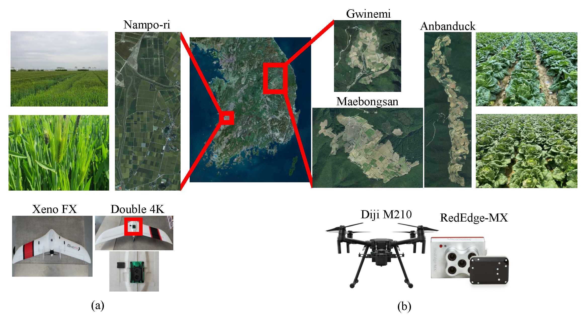
3.1. UAV Image Acquisition

We acquired UAV images from four target sites located in two provinces in South Korea, which are three highland areas used for cultivating kimchi cabbage and one plain used for cultivating barley, as shown in Figure 5. Kimchi cabbage is the primary vegetable that affects consumer prices in South Korea and, therefore, accurate yield prediction is essential. Table A1 summarizes the details of the image acquisition.

3.2. Preprocessing Dataset

Creating Wide-Area Image Mosaics. We performed postprocessing steps to create wide-area image mosaics from the acquired UAV images. To create a mosaic of high quality, it is necessary to ensure that images are continuously acquired from a single flight of UAV. For this purpose, we set the flight trajectory of a single UAV flight conditioned on the overlap threshold of 0.7 in terms of intersection over union (IoU). When performing mosaicking, images acquired during takeoff and landing were excluded. We used commercial software, PIX4D Mapper [56] for stitching UAV images. The process of mosaicking uses simple image stitching with no orthorectification. Examples of the mosaics are shown in Figure 6. The details of the image mosaicking process are presented in Table A1.
Annotation of Reference Points. After creating the mosaics, reference points of datasets on the kimchi cabbage-cultivating highland (datasets D A , D B , and D C in Table A1) were annotated by carefully identifying time-invariant and visually distinguishable locations such as warehouse and road junctions (see Figure 6 for examples). We created 200 reference points for each image mosaic in dataset D A , D B , and D C , and 100 reference points for each image mosaic in dataset D D . In addition, for dataset D D , we separately annotated 20 RTK-based GCPs as an alternative set of reference points.

3.3. Case Studies on Local Alignment

We adopt three algorithms for the local alignment: RANSAC, moving direct linear transformation algorithm, or MDLT [57] and DNN-based method, called RANSAC-flow [48]. The application of RANSAC to the local alignment is straightforward; it is identical to the global alignment except that we calculate individual homographies for each patch only with their corresponding keypoints.
On the contrary, RANSAC-flow predicts the transformation of each pixel in a nonparametric way, called flow, in the matchable regions of the input images by exploiting features of a neural network. In the local alignment step, RANSAC-flow estimates the flow between two patches from the source and target mosaics. We exploit these flows instead of matched keypoints when estimating individual mapping between the patches. MDLT estimates each patch-level homography by using weighted singular value decomposition (SVD), where the distance between keypoints and the center of the patch is explicitly considered, similar to ours. MDLT is a single-stage approach, directly calculating the homography of each patch without needing the global alignment. Those homographies correspond to the local alignment of the proposed method. However, calculating a patch’s homography requires the entire keypoints of an input mosaic. As a result, local homographies are not entirely independent.

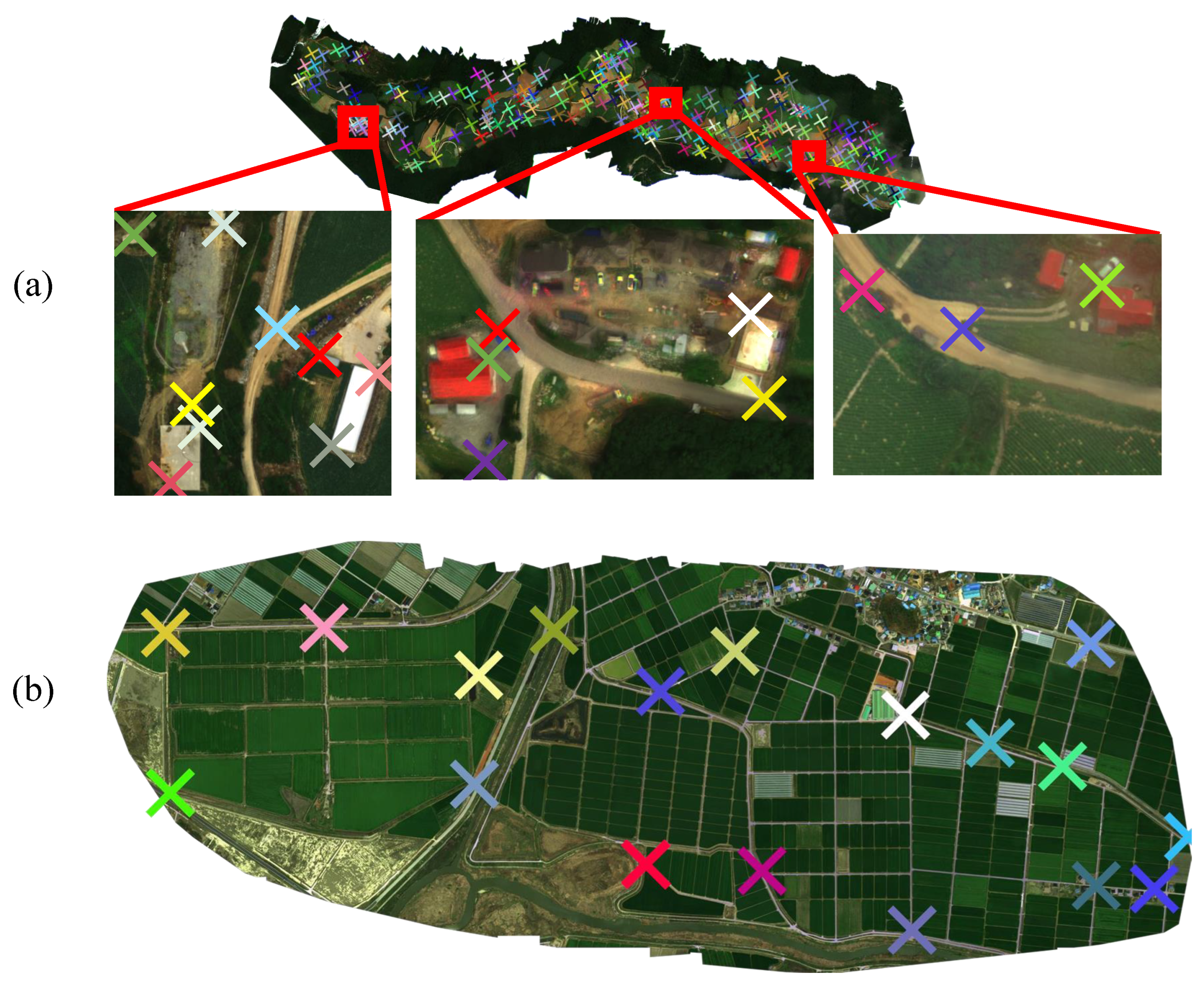
3.4. Evaluation Metric

We measure alignment accuracy using the Euclidean distance between two sets of reference points annotated in X s and X t . The distance function d ( · , · ) in Equation (1) for R s = { r s ( i ) } and R t = { r t ( i ) } is given as
d R s , R t = 1 | R s | i | R t | r s ( i ) r t ( i ) .

3.5. Method Implementations

We used a DNN-based method to extract keypoints from the input mosaic images [42]. From an input image, the keypoint extractor evaluates two types of confidence scores, repeatability and reliability, of pixels as its eligibility for being keypoints. Repeatability corresponds to how robust keypoints appear over images, whereas reliability corresponds to how strong a keypoint is among candidates in the images. Pixels with high values of the scores are likely to be keypoints. We use a threshold on the scores to control the number of keypoints and obtain keypoints of high quality, which is investigated in Section 4.2. We set the dimension of a keypoint descriptor φ ( · ) to 128. The input mosaics are fed into patches of 1024 × 1024 px as inputs of the keypoint extractor. Table A2 shows the summary of the keypoint extractions.
In the local alignment, we divide the source and target mosaics into patches so that corresponding geographical areas are similar. In particular, we used patches of 2000 × 2000 px for D A , D B , and D C and 3000 × 3000 px for D D considering its smaller ground sample distance (GSD) (the distance between pixels measured on the ground), compared with that of other datasets, letting the local alignment take the similar area as inputs from the datasets. The threshold to pixel distance τ l to choose outlier keypoint pairs, discussed in Section 2.3, was set differently, which was τ l = 50 for datasets D A , D B , and D C and τ l = 100 for dataset D D , respectively.
We implemented an in-house tool for annotating reference keypoints and the proposed alignment framework in Python. We used open-sourced Python implementations for MDLT and RANSAC-flow [48,57], which have been integrated into our framework.

4. Results and Discussions

4.1. Performance Comparisons

We first compare the performance of several methods to assess the effects of the components of the proposed method on the alignment accuracy. In particular, we consider several variants of the proposed method as shown in Table 2; “Global” and “G + reference points” perform the global alignment only. They differ in that “Global” uses the extracted keypoints, i.e., C t and C s , whereas “G + reference points” uses the reference points R t and R s as keypoints for finding mapping m g . Moreover, “G + RANSAC” and “G + RANSAC-flow” involve the local alignments without boundary-aware alignment, which are RANSAC and RANSAC-flow, respectively. The last two variants, “G + RANSAC+BA” and “G + RANSAC-flow + BA”, perform the local alignment step with boundary-aware alignment (BA).
Table 2 summarizes the average alignment errors for each dataset. The alignment errors of each mosaic image are listed in Table A2 and Table A3. We first observe that our method outperforms MDLT across all the datasets; for example, by 13.21% in dataset D B and 7.06% in dataset D C , respectively. In the proposed method, local transformations for subregions tend to be independent of a global transformation, leading to nontrivial performance improvements from the results of the global alignment. On the other hand, given that local transformations with “MDLT” strongly correlate with a global transformation, “MDLT” provides trivial performance improvement compared with “Global” by 0.18–2.4% over the datasets.
Moreover, despite the reference points being manually and carefully annotated for evaluating methods, the difference in alignment accuracy between the usage of reference points for the global alignment, “G + reference points”, and extracted keypoints, “Global”, is negligible except D D . This observation implies that DNN-based keypoint extraction provides high-quality keypoints essential to achieving accurate alignment.
We evaluate how the local alignment step affects the accuracy of the proposed method through two variants, “G + RANSAC” and “G + RANSAC-flow”. Applying local alignments without the global alignment is infeasible because no geographic similarity between patches of the source and target images is known before the global alignment. The DNN-based alignment, “G + RANSAC-Flow”, outweighs the conventional method, “G + RANSAC”, across all datasets by 4.7–18.9%. However, there exist several tradeoffs for using DNNs in the local alignment. In RANSAC-flow, the flow estimation considers the relationship between all pixels, resulting in more reliable and denser pixel-level correspondences. However, in terms of applicability and flexibility, conventional methods can consider the arbitrary form of keypoints created by human intervention or from external techniques exploiting rich positional information. Furthermore, conventional methods can reuse keypoints used in the global alignment. On the other hand, DNN-based methods typically extract keypoints based on their internal representation with the extra time cost.
Finally, the last two rows show that the proposed method with the different local alignments eliminated the boundary artifacts effectively, as shown in Figure 7. Even though the lack of boundary-aware alignment in the local alignment step leads to superior performance compared with their counterparts using boundary-aware alignment, these performance gains arise from the fact that the accuracy metric is only concerned with the distance between the reference points, unaware of the visual fidelity of a transformed image. The artifacts at boundaries are more obvious when the distance between the homographies corresponding to two adjacent patches grows. Figure 7 depicts sampled results of the proposed method “G + RANSAC + BA” that shows a natural-looking alignment as a compromise at the expense of a slight sacrifice of accuracy. The visual insusceptibility at boundaries can be crucial to downstream tasks needing the mosaics. For instance, field usage identification with respect to cultivated crops may be deteriorated if the artifacts exist, which is clearly shown in the example in the right column of the second row in Figure 7.

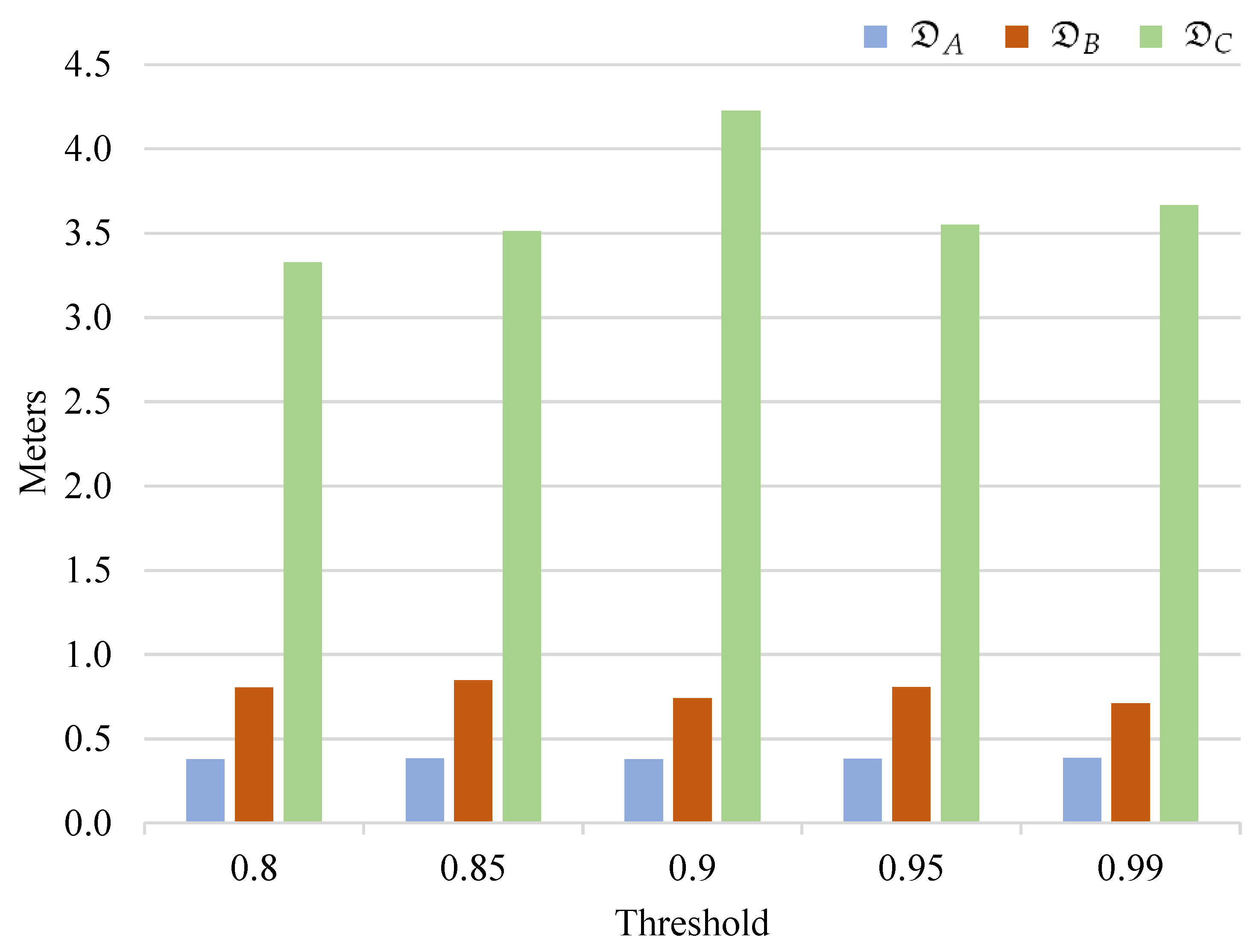
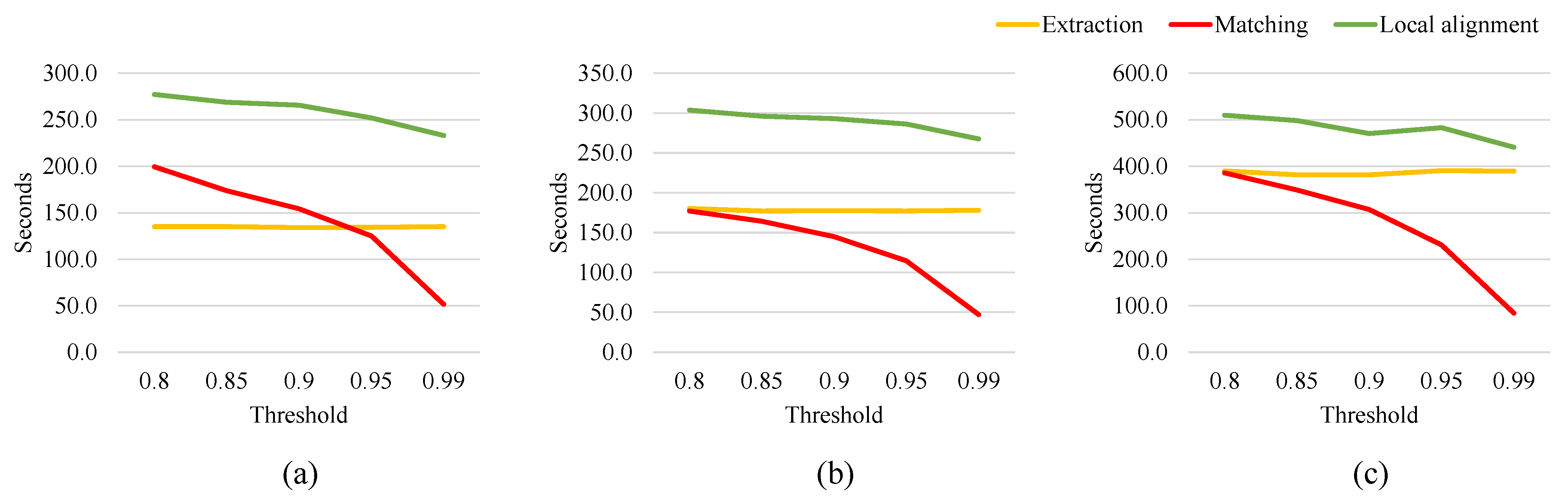
4.2. Effects of the Number of Keypoints on Accuracy and Speed

Despite the promising performance, the DNN-based method, RANSAC-flow relies on the implicit internal information instead of explicit keypoints for local alignments, resulting in its limited applicability in case of handling images deviated from its training data. In contrast, RANSAC requires at least four keypoint pairs to estimate homography. We contemplate how the number of keypoints, | C t | and | C s | , affects the accuracy and speed of the proposed method. We note that from the alignment speed perspective, the time for keypoint extraction is nearly consistent as long as the resolutions of an input patch are kept. However, the time for matching keypoint pairs in Equation (6) depends on both | C t | and | C s | with time complexity of O C t · C s .
Table 3 and Figure 8 and Figure 9 depict the aforementioned tradeoff to determine the optimal number of keypoints. As explained in Section 3.2, using a higher threshold value for the keypoint scores when extracting keypoints ends in a smaller number of keypoints as shown in Table 3. A lower threshold value results in a larger number of keypoints, likely to include a larger number of poor keypoints that must be excluded as outliers. Moreover, increasing the number of keypoints requires a longer processing time for keypoint extraction and matching, as shown in Figure 9. In particular, time for the keypoint matching dominates the entire processing time and decreases superlinearly to the number of keypoints. We chose 0.99 as the threshold of the keypoint score. Although an excessively high threshold may result in the extraction of an insufficient number of keypoints and omission of essential keypoints, nearly consistent alignment errors in Figure 8 suggest that no such side effects were found in our cases.

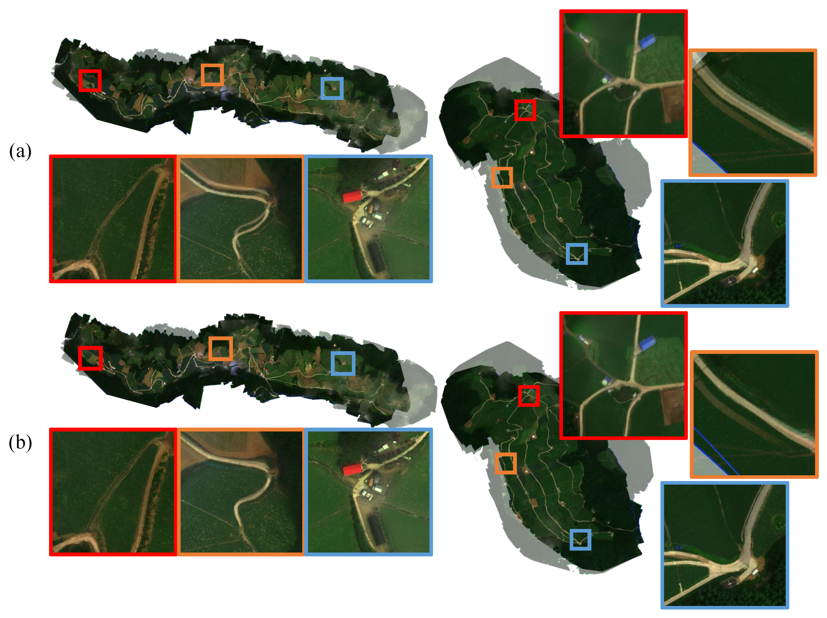
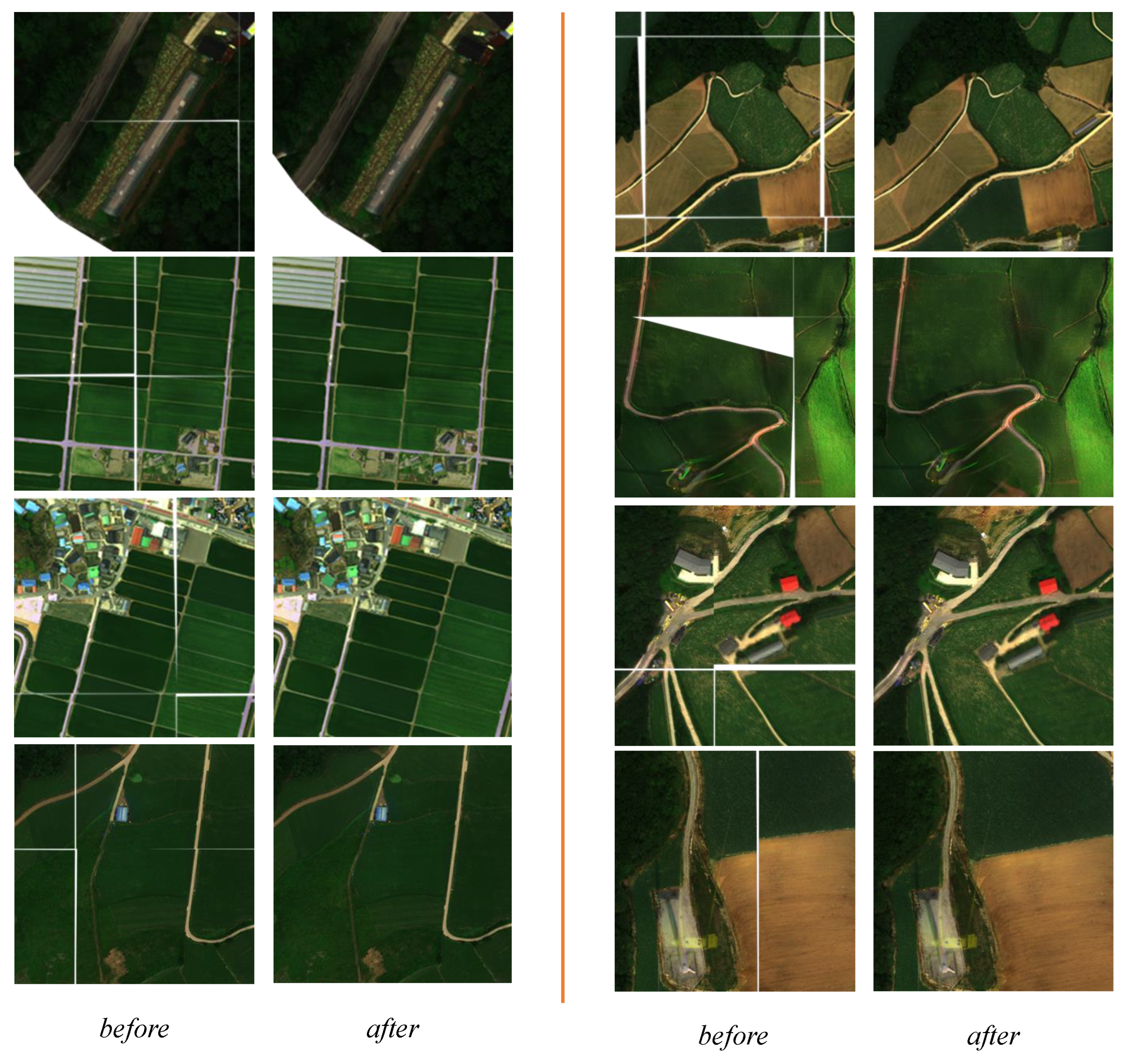
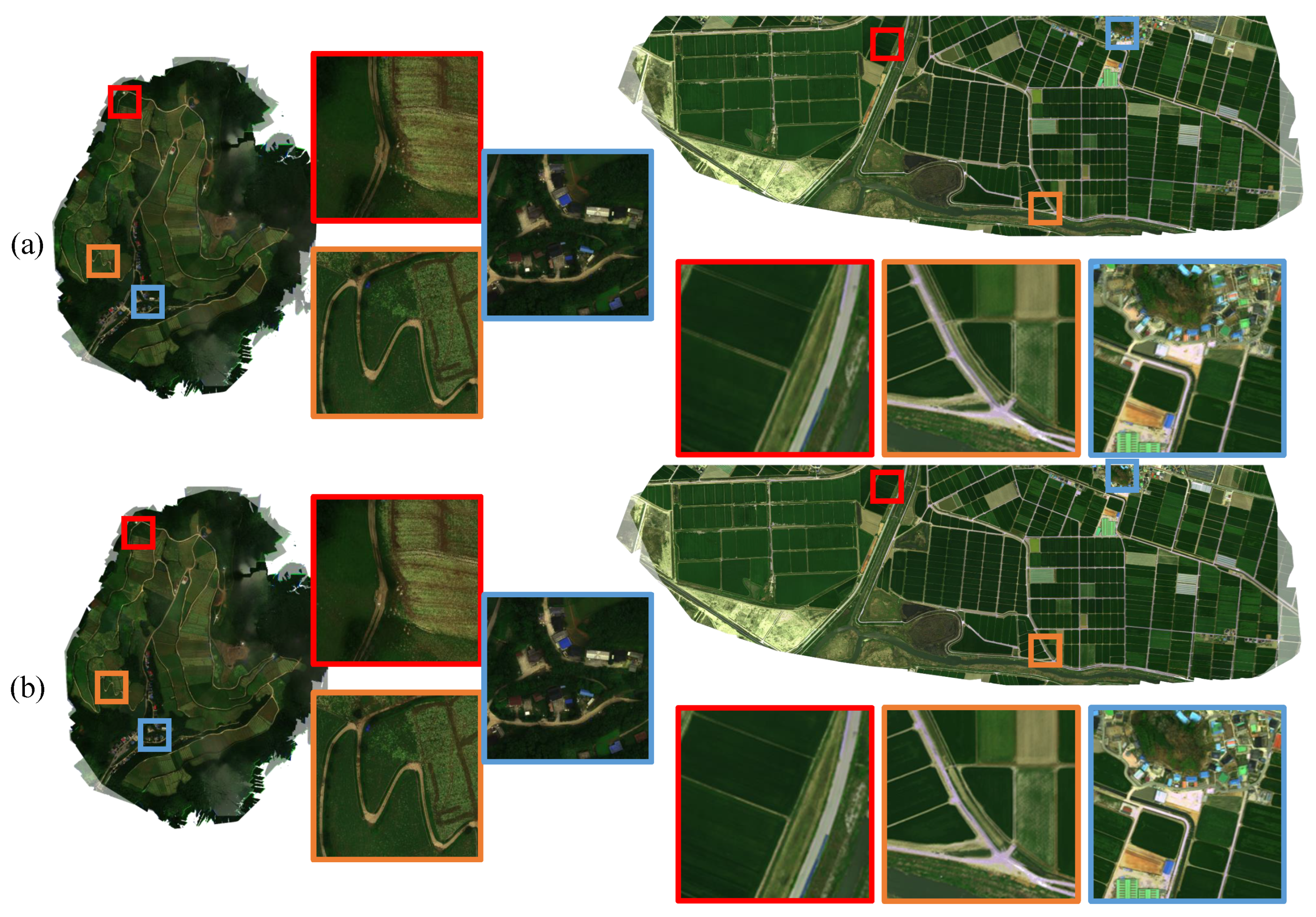
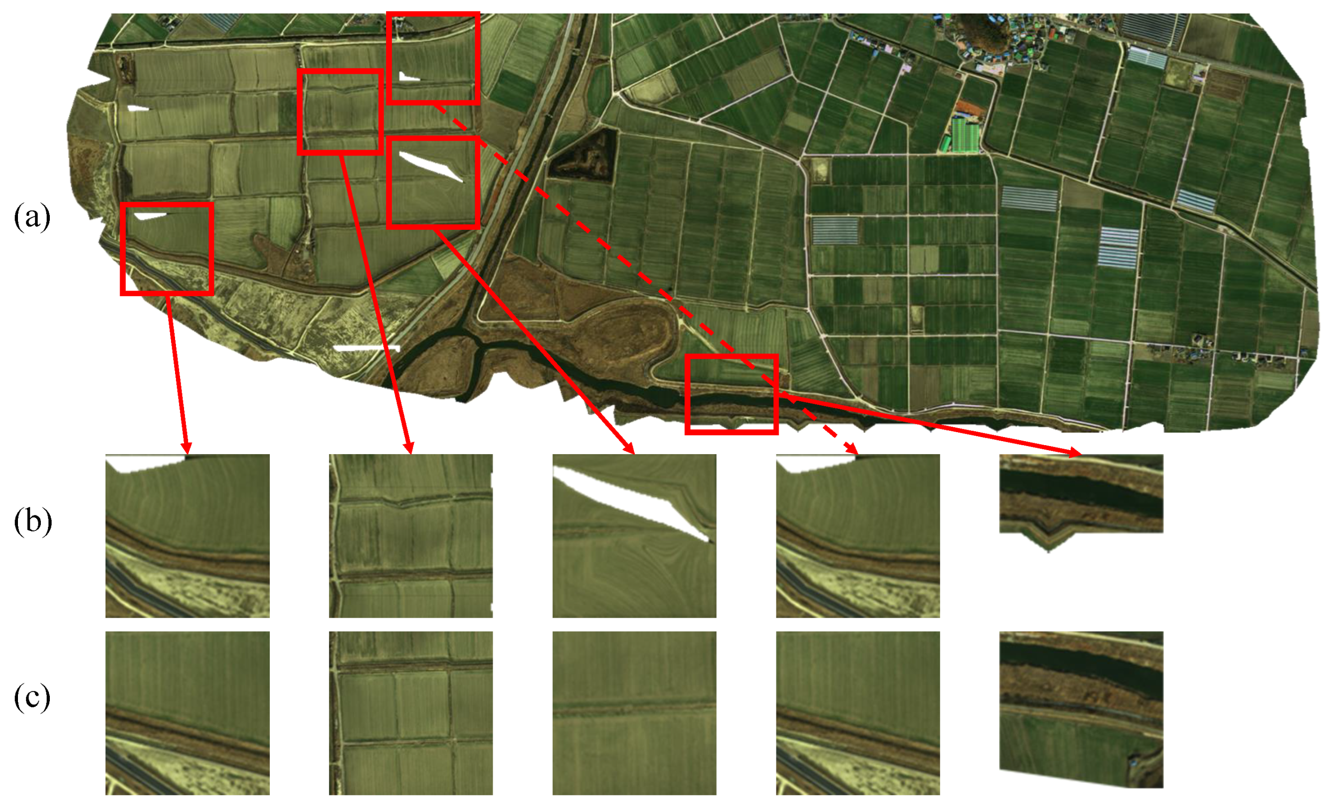
4.3. Qualitative Evaluations

Figure 10 and Figure 11 show that the proposed local alignment step alleviates misalignments effectively, which is untapped by the global alignment. For ease of comparison, X s and X t overlap, and the opacity of the target is set to 0.5. We highlight patches containing significant misalignments even with the global alignment. Structured objects, such as buildings and roads, appear redundantly, or the regions look blurry, and they are resolved by the proposed method.
We also show the benefits of boundary-aware alignment in Figure 7. We sampled 10 regions in the mosaics 190,828, 190,909, 190,724, and 210,427 from datasets D A , D B , D C , and D D , respectively, and provide the results of the local alignment when applying boundary-aware alignment. Severe boundary artifacts appear owing to the application of independent homographies to patches without boundary-aware alignment.
Not all boundary artifacts can be eliminated from boundary-aware alignment. In particular, due to the nondeterministic nature of sampling keypoint pairs in RANSAC, an outlier may deteriorate homography estimation. Moreover, inputs deviating from the distribution of training data may confuse the DNN-based alignment and result in incorrect alignment predictions. In our experiments, the first issue rarely occurred because the keypoint matching in the local alignment is based on geometric proximity between keypoints. Still, the second issue has not been fully addressed, as shown in Figure 12. Section 4.4 discusses this limitation of DNN-based alignments.

4.4. Discussions for Improving the Proposed Method

We demonstrated the viability of the proposed method in terms of alignment accuracy and practical applicability. There is still room for improvement. This section discusses several limitations of our method and addresses future directions.
Dataset Requirements for Training Keypoint Extractor. The alignment accuracy of the proposed method largely depends on the quality of keypoints. The keypoint extractor used in this study was trained with a dataset containing various natural scenes. Because such a dataset may have different characteristics for extracting keypoints compared with typical UAV images of farmland, keypoint extraction can be improved if the extractor is further trained with a dataset tailored for this purpose, which requires substantial engineering efforts as discussed below.
Inconsistent Keypoint Extraction Caused by Time-Variant Image Patterns. Extracting keypoints of high quality assumes that images possess time-invariant texture patterns. However, UAV images of farmland may vary based on environmental changes, such as a quick shift in weather conditions or fast crop growth. As a result, more outlier keypoints are likely to appear, as shown in Figure 13. To address this problem, the keypoint extraction must be trained to focus on time-invariant patterns—for example, the unique shapes of roads, warehouses, and other facilities. The use of multispectral images that contain invisible wavelength ranges may help this purpose.
Furthermore, when a patch has less than four keypoint pairs, the proposed method retains the global alignment. If any misalignments are present in the patch, they remain untapped, as shown in Figure 13. Possible solutions to this problem would be to encourage the extraction of keypoints across all patches in the mosaic or apply interpolated homographies of neighboring patches to a patch with sparse keypoints.
Misalignments Near Patch Boundaries. While the proposed method effectively alleviates the problem of boundary artifacts, remaining misaligned keypoints from the global alignment may be untapped if they are close to patch boundaries because they are hardly affected by transformations applied in the local alignment. A possible solution to the problem is to consider mixing homoghrapies of two adjacent patches as a transformation applied to patch boundary regions. Another method is to determine the patch boundaries by selecting areas with few keypoints if the keypoints distribution is nonuniform.

5. Conclusions

This study proposed a simple yet effective method to align high-resolution, wide-area mosaic images through two steps, global and local alignments. The global alignment aims to align the source and target mosaics on the whole by applying a single homography using keypoints pairs created from a DNN-based extractor. Then the second step, the local alignment, improves the alignment by removing the local misalignments within small patches obtained by dividing the mosaics with their transformations. Although the local alignment results in better accuracy than the global alignment, new artifacts at patch boundaries may be introduced, which degrades the perceptual quality and applicability of the final alignment. To overcome this problem, we introduced a novel technique, called boundary-aware alignment, to preserve boundary consistency between adjacent patches while improving local alignments. We demonstrated the effectiveness of the proposed method on wide-area mosaics acquired from four representative regions cultivating kimchi cabbage and barley in South Korea. The experiments showed that integrating two steps resulted in the best alignment accuracy across all datasets. The alignment errors ranged from 0.46 to 2.46 m, which is an improvement of by up to 13.21% over recent approaches.

Author Contributions

Conceptualization, H.L. and S.K. (Sungchan Kim); methodology, H.L. and S.K. (Sungchan Kim); software, H.L.; formal analysis, H.L. and S.K. (Sungchan Kim); investigation, S.K. (Semo Kim) and L.-H.K.; resources, S.-H.B., L.-H.K. and S.K. (Sungchan Kim); data curation, S.K. (Semo Kim), D.L., S.-H.B. and L.-H.K.; writing—original draft, H.L.; writing—review & editing, S.K. (Sungchan Kim); supervision, L.-H.K. and S.K. (Sungchan Kim); project administration, S.-H.B., L.-H.K. and S.K. (Sungchan Kim); funding acquisition, S.-H.B., L.-H.K. and S.K. (Sungchan Kim). All authors have read and agreed to the published version of the manuscript.

Funding

This work was supported by the Spatial Information Research Institute grant funded by LX (Grant No. 2020-502) and the National Research Foundation of Korea (NRF) grant funded by the Korea government (MSIT) (No. 2022R1A2C1011013).

Institutional Review Board Statement

Not applicable.

Informed Consent Statement

Not applicable.

Data Availability Statement

Not applicable.

Conflicts of Interest

The authors declare no conflict of interest.

Appendix A

Table A1. Information on UAV image acquisition. The acquisition frequency of dataset D D was varied such that the overlap ratio of consecutive images is no smaller than 65%.
Dataset D A D B D C D D
Study siteAnbanduckGwinemiMaebongsanNampo-ri
Provincial locationGangwonGangwonGangwonJeollabuk
Geographic longitudeN 37°13′05″N 37°20′21″N 37°37′31″N 35°48′20″
Geographic latitudeE 128°57′58″E 129°00′20″E 128°44′21″E 126°46′55″
Area of study site
(km2)
8.552.183.853.77
CropsKimchi cabbageKimchi cabbageKimchi cabbageBarley
Dates of acquisition
(yymmdd)
190725, 190809,
190828, 190909
190807, 190809,
190902, 190909
190724, 190729,
190805, 190808
210223, 210323,
210415, 210420,
210427, 210506,
210518, 210525,
210609
UAV model usedDJI M210
(rotary wing)
DJI M210DJI M210Xeno FX
(fixed wing)
Image sensor usedRedEdge-MX
(MicaSense)
RedEdge-MXRedEdge-MXDouble 4K
(Sentera)
Flight altitude123510751235300
UAV Image resolution
(width × height)
1280 × 9601280 × 9601280 × 9604000 × 3000
Ground sampling distance13.5811.9713.818.14
Acquisition frequency
(frames/s)
222Variable
Average mosaic resolution
(width × height × channel)
11,973 × 38,023 × 3 (RGB)11,075 × 13,941 × 317,037 × 11,982 × 339,817 × 14,431 × 3
# images for mosaicking197,666932511,227623
# reference points
(Annotation method)
268
(Manually)
338
(Manually)
260
(Manually)
100
(Manually + GCP)
Table A2. Keypoints used in the datasets.
DatasetSource# KPs in Global
Alignment ( × 10 6 )
# Patches# KPs/Patch in
Local Alignment
# GCPs
D A 1907252.09120--
1908093.04120142.51-
1908282.93133276.95-
1909092.26133197.92-
D B 1908071.3042--
1908091.564822,048-
1909021.7042434.02-
1909091.7248371.96-
D C 1907291.2654--
1907240.97542189.13-
1908050.9763105.16-
1908081.9163115.16-
D D 2105061.1370--
2102231.23780.5420
2103231.13650.906-
2104151.298414.4120
2104201.408422.45-
2104271.408481.6-
2105181.13703.48-
2105251.32701.02-
2106091.02703.2620
Table A3. Results of case studies. Alignments errors are shown in meter unless specified otherwise. Less errors represent better alignment performance.
DatasetSourceGlobal (G)G + Ref.G + RANSAC (LR)G + LR + BA
D A 1908282.352.491.832.26
1909092.582.612.102.58
avg. error2.542.542.022.46
avg. error (pixels)18.7218.7114.8518.12
D B 1909020.720.710.560.48
1909090.350.350.320.35
avg. error0.620.610.420.46
avg. error (pixels)5.145.113.493.88
D C 1908050.921.000.650.88
1908080.850.900.640.84
avg. error0.870.910.620.79
avg. error (pixels)6.286.594.465.69
D D 2102232.821.022.822.82
2103230.731.060.750.73
2104151.021.330.760.84
2104200.740.910.610.64
2104270.780.790.560.69
2105181.330.931.271.25
2105251.010.901.011.01
2106090.991.340.940.94
avg. error1.181.041.091.12
avg. error (pixels)14.4612.7313.3613.73

References

  1. Colomina, I.; Molina, P. Unmanned aerial systems for photogrammetry and remote sensing: A review. ISPRS J. Photogramm. Remote Sens. 2014, 92, 79–97. [Google Scholar] [CrossRef]
  2. Zhou, X.; Zheng, H.; Xu, X.; He, J.; Ge, X.; Yao, X.; Cheng, T.; Zhu, Y.; Cao, W.; Tian, Y. Predicting grain yield in rice using multi-temporal vegetation indices from UAV-based multispectral and digital imagery. ISPRS J. Photogramm. Remote Sens. 2017, 130, 246–255. [Google Scholar] [CrossRef]
  3. Kim, J.I.; Kim, H.C.; Kim, T. Robust Mosaicking of Lightweight UAV Images Using Hybrid Image Transformation Modeling. Remote Sens. 2020, 12, 1002. [Google Scholar] [CrossRef]
  4. Jannoura, R.; Brinkmann, K.; Uteau, D.; Bruns, C.; Joergensen, R.G. Monitoring of crop biomass using true colour aerial photographs taken from a remote controlled hexacopter. Biosyst. Eng. 2015, 129, 341–351. [Google Scholar] [CrossRef]
  5. Jay, S.; Baret, F.; Dutartre, D.; Malatesta, G.; Héno, S.; Comar, A.; Weiss, M.; Maupas, F. Exploiting the centimeter resolution of UAV multispectral imagery to improve remote-sensing estimates of canopy structure and biochemistry in sugar beet crops. Remote Sens. Environ. 2019, 231, 110898. [Google Scholar] [CrossRef]
  6. Feng, A.; Zhou, J.; Vories, E.D.; Sudduth, K.A.; Zhang, M. Yield estimation in cotton using UAV-based multi-sensor imagery. Biosyst. Eng. 2020, 193, 101–114. [Google Scholar] [CrossRef]
  7. Fernandez-Gallego, J.A.; Kefauver, S.C.; Vatter, T.; Gutiérrez, N.A.; Nieto-Taladriz, M.T.; Araus, J.L. Low-cost assessment of grain yield in durum wheat using RGB images. Eur. J. Agron. 2019, 105, 146–156. [Google Scholar] [CrossRef]
  8. Walter, J.; Edwards, J.; McDonald, G.; Kuchel, H. Photogrammetry for the estimation of wheat biomass and harvest index. Field Crops Res. 2018, 216, 165–174. [Google Scholar] [CrossRef]
  9. Sofonia, J.; Shendryk, Y.; Phinn, S.; Roelfsema, C.; Kendoul, F.; Skocaj, D. Monitoring sugarcane growth response to varying nitrogen application rates: A comparison of UAV SLAM LiDAR and photogrammetry. Int. J. Appl. Earth Obs. Geoinf. 2019, 82, 101878. [Google Scholar] [CrossRef]
  10. Jensen, A.M.; Baumann, M.; Chen, Y. Low-cost multispectral aerial imaging using autonomous runway-free small flying wing vehicles. In Proceedings of the IGARSS 2008—2008 IEEE International Geoscience and Remote Sensing Symposium, Boston, MA, USA, 6–11 July 2008; IEEE: New York, NY, USA, 2008; Volume 5, p. V-506. [Google Scholar]
  11. Zhang, C.; Kovacs, J.M. The application of small unmanned aerial systems for precision agriculture: A review. Precis. Agric. 2012, 13, 693–712. [Google Scholar] [CrossRef]
  12. Khaki, S.; Wang, L. Crop yield prediction using deep neural networks. Front. Plant Sci. 2019, 10, 621. [Google Scholar] [CrossRef]
  13. Gil-Yepes, J.L.; Ruiz, L.A.; Recio, J.A.; Balaguer-Beser, Á.; Hermosilla, T. Description and validation of a new set of object-based temporal geostatistical features for land-use/land-cover change detection. ISPRS J. Photogramm. Remote Sens. 2016, 121, 77–91. [Google Scholar] [CrossRef]
  14. van Deventer, H.; Cho, M.A.; Mutanga, O. Multi-season RapidEye imagery improves the classification of wetland and dryland communities in a subtropical coastal region. ISPRS J. Photogramm. Remote Sens. 2019, 157, 171–187. [Google Scholar] [CrossRef]
  15. Alibabaei, K.; Gaspar, P.D.; Lima, T.M. Crop Yield Estimation Using Deep Learning Based on Climate Big Data and Irrigation Scheduling. Energies 2021, 14, 3004. [Google Scholar] [CrossRef]
  16. Khaki, S.; Wang, L.; Archontoulis, S.V. A cnn-rnn framework for crop yield prediction. Front. Plant Sci. 2020, 10, 1750. [Google Scholar] [CrossRef] [PubMed]
  17. Xingjian, S.; Chen, Z.; Wang, H.; Yeung, D.Y.; Wong, W.K.; Woo, W.C. Convolutional LSTM network: A machine learning approach for precipitation nowcasting. In Proceedings of the Advances in Neural Information Processing Systems, Montreal, QC, Canada, 7–12 December 2015; pp. 802–810. [Google Scholar]
  18. Ji, S.; Zhang, C.; Xu, A.; Shi, Y.; Duan, Y. 3D convolutional neural networks for crop classification with multi-temporal remote sensing images. Remote Sens. 2018, 10, 75. [Google Scholar] [CrossRef]
  19. Pelletier, C.; Webb, G.I.; Petitjean, F. Temporal convolutional neural network for the classification of satellite image time series. Remote Sens. 2019, 11, 523. [Google Scholar] [CrossRef]
  20. Lai, Y.; Pringle, M.; Kopittke, P.M.; Menzies, N.W.; Orton, T.G.; Dang, Y.P. An empirical model for prediction of wheat yield, using time-integrated Landsat NDVI. Int. J. Appl. Earth Obs. Geoinf. 2018, 72, 99–108. [Google Scholar]
  21. Xu, Z.; Guan, K.; Casler, N.; Peng, B.; Wang, S. A 3D convolutional neural network method for land cover classification using LiDAR and multi-temporal Landsat imagery. ISPRS J. Photogramm. Remote Sens. 2018, 144, 423–434. [Google Scholar] [CrossRef]
  22. Fernandez-Manso, A.; Quintano, C.; Roberts, D.A. Burn severity analysis in Mediterranean forests using maximum entropy model trained with EO-1 Hyperion and LiDAR data. ISPRS J. Photogramm. Remote Sens. 2019, 155, 102–118. [Google Scholar] [CrossRef]
  23. Galin, E.; Guérin, E.; Peytavie, A.; Cordonnier, G.; Cani, M.P.; Benes, B.; Gain, J. A review of digital terrain modeling. In Proceedings of the Computer Graphics Forum, Genoa, Italy, 6–10 May 2019; Volume 38, pp. 553–577. [Google Scholar]
  24. Habib, A.F.; Kim, E.M.; Kim, C.J. New methodologies for true orthophoto generation. Photogramm. Eng. Remote Sens. 2007, 73, 25–36. [Google Scholar] [CrossRef]
  25. Demiray, B.Z.; Sit, M.; Demir, I. D-SRGAN: DEM super-resolution with generative adversarial networks. SN Comput. Sci. 2021, 2, 48. [Google Scholar] [CrossRef]
  26. Panagiotou, E.; Chochlakis, G.; Grammatikopoulos, L.; Charou, E. Generating Elevation Surface from a Single RGB Remotely Sensed Image Using Deep Learning. Remote Sens. 2020, 12, 2002. [Google Scholar] [CrossRef]
  27. Väänänen, P. Removing 3D Point Cloud Occlusion Artifacts with Generative Adversarial Networks. Ph.D. Thesis, Department of Computer Science, University of Helsinki, Helsinki, Findland, 2019. [Google Scholar]
  28. Huang, H.; Deng, J.; Lan, Y.; Yang, A.; Zhang, L.; Wen, S.; Zhang, H.; Zhang, Y.; Deng, Y. Detection of helminthosporium leaf blotch disease based on UAV imagery. Appl. Sci. 2019, 9, 558. [Google Scholar] [CrossRef]
  29. de Souza, C.H.W.; Mercante, E.; Johann, J.A.; Lamparelli, R.A.C.; Uribe-Opazo, M.A. Mapping and discrimination of soya bean and corn crops using spectro-temporal profiles of vegetation indices. Int. J. Remote Sens. 2015, 36, 1809–1824. [Google Scholar] [CrossRef]
  30. Nevavuori, P.; Narra, N.; Linna, P.; Lipping, T. Crop yield prediction using multitemporal UAV data and spatio-temporal deep learning models. Remote Sens. 2020, 12, 4000. [Google Scholar] [CrossRef]
  31. Malambo, L.; Popescu, S.C.; Murray, S.C.; Putman, E.; Pugh, N.A.; Horne, D.W.; Richardson, G.; Sheridan, R.; Rooney, W.L.; Avant, R.; et al. Multitemporal field-based plant height estimation using 3D point clouds generated from small unmanned aerial systems high-resolution imagery. Int. J. Appl. Earth Obs. Geoinf. 2018, 64, 31–42. [Google Scholar] [CrossRef]
  32. Varela, S.; Varela, S.; Leakey, A.D.; Leakey, A.D. Implementing spatio-temporal 3D-convolution neural networks and UAV time series imagery to better predict lodging damage in sorghum. AgriRxiv 2022, 20220024994. [Google Scholar] [CrossRef]
  33. Yu, M.; Wu, B.; Yan, N.; Xing, Q.; Zhu, W. A method for estimating the aerodynamic roughness length with NDVI and BRDF signatures using multi-temporal Proba-V data. Remote Sens. 2016, 9, 6. [Google Scholar] [CrossRef]
  34. Kim, D.H.; Yoon, Y.I.; Choi, J.S. An efficient method to build panoramic image mosaics. Pattern Recognit. Lett. 2003, 24, 2421–2429. [Google Scholar] [CrossRef]
  35. Lowe, D.G. Distinctive image features from scale-invariant keypoints. Int. J. Comput. Vis. 2004, 60, 91–110. [Google Scholar] [CrossRef]
  36. Moussa, A.; El-Sheimy, N. A Fast Approach for Stitching of Aerial Images. Int. Arch. Photogramm. Remote Sens. Spat. Inf. Sci. 2016, 41, 769–774. [Google Scholar] [CrossRef]
  37. Faraji, M.R.; Qi, X.; Jensen, A. Computer vision–based orthorectification and georeferencing of aerial image sets. J. Appl. Remote Sens. 2016, 10, 036027. [Google Scholar] [CrossRef]
  38. Zhang, W.; Guo, B.; Li, M.; Liao, X.; Li, W. Improved seam-line searching algorithm for UAV image mosaic with optical flow. Sensors 2018, 18, 1214. [Google Scholar] [CrossRef] [PubMed]
  39. Li, L.; Yao, J.; Xie, R.; Li, J. Edge-enhanced optimal seamline detection for orthoimage mosaicking. IEEE Geosci. Remote Sens. Lett. 2018, 15, 764–768. [Google Scholar] [CrossRef]
  40. Fang, F.; Wang, T.; Fang, Y.; Zhang, G. Fast color blending for seamless image stitching. IEEE Geosci. Remote Sens. Lett. 2019, 16, 1115–1119. [Google Scholar] [CrossRef]
  41. Jaderberg, M.; Simonyan, K.; Zisserman, A.; Kavukcuoglu, K. Spatial transformer networks. arXiv 2015, arXiv:1506.02025. [Google Scholar]
  42. Revaud, J.; Weinzaepfel, P.; De Souza, C.; Pion, N.; Csurka, G.; Cabon, Y.; Humenberger, M. R2D2: Repeatable and reliable detector and descriptor. arXiv 2019, arXiv:1906.06195. [Google Scholar]
  43. DeTone, D.; Malisiewicz, T.; Rabinovich, A. Superpoint: Self-supervised interest point detection and description. In Proceedings of the IEEE Conference on Computer Vision and Pattern Recognition Workshops, Salt Lake City, UT, USA, 18–22 June 2018; pp. 224–236. [Google Scholar]
  44. Christiansen, P.H.; Kragh, M.F.; Brodskiy, Y.; Karstoft, H. Unsuperpoint: End-to-end unsupervised interest point detector and descriptor. arXiv 2019, arXiv:1907.04011. [Google Scholar]
  45. Sarlin, P.E.; DeTone, D.; Malisiewicz, T.; Rabinovich, A. Superglue: Learning feature matching with graph neural networks. In Proceedings of the IEEE/CVF Conference on Computer Vision and Pattern Recognition, Online, 14–19 June 2020; pp. 4938–4947. [Google Scholar]
  46. Yuan, Y.; Fang, F.; Zhang, G. Superpixel-Based Seamless Image Stitching for UAV Images. IEEE Trans. Geosci. Remote Sens. 2021, 59, 1565–1576. [Google Scholar] [CrossRef]
  47. Li, L.; Xia, M.; Liu, C.; Li, L.; Wang, H.; Yao, J. Jointly optimizing global and local color consistency for multiple image mosaicking. ISPRS J. Photogramm. Remote Sens. 2020, 170, 45–56. [Google Scholar] [CrossRef]
  48. Shen, X.; Darmon, F.; Efros, A.A.; Aubry, M. Ransac-flow: Generic two-stage image alignment. In Proceedings of the Computer Vision–ECCV 2020: 16th European Conference, Glasgow, UK, 23–28 August 2020; Part IV 16. Springer: Online, 2020; pp. 618–637. [Google Scholar]
  49. Fischler, M.A.; Bolles, R.C. Random sample consensus: A paradigm for model fitting with applications to image analysis and automated cartography. Commun. ACM 1981, 24, 381–395. [Google Scholar] [CrossRef]
  50. Duda, R.O.; Hart, P.E. Use of the Hough transformation to detect lines and curves in pictures. Commun. ACM 1972, 15, 11–15. [Google Scholar] [CrossRef]
  51. Rosenfeld, A.; Pfaltz, J.L. Distance functions on digital pictures. Pattern Recognit. 1968, 1, 33–61. [Google Scholar] [CrossRef]
  52. National Geographic Information Institute. Available online: http://map.ngii.go.kr/ (accessed on 23 December 2022).
  53. Korea Rural Economic Institute. Available online: https://aglook.krei.re.kr/ (accessed on 23 December 2022).
  54. SZ DJI Technology Company, Limited. Available online: https://www.dji.com/ (accessed on 23 December 2022).
  55. MicaSense, Incorporated. Available online: https://micasense.com/ (accessed on 23 December 2022).
  56. PIX4Dmapper. Available online: https://www.pix4d.com/product/pix4dmapper-photogrammetry-software/ (accessed on 23 December 2022).
  57. Zaragoza, J.; Chin, T.J.; Brown, M.S.; Suter, D. As-projective-as-possible image stitching with moving DLT. In Proceedings of the IEEE Conference on Computer Vision and Pattern Recognition, Portland, OR, USA, 23–28 June 2013; pp. 2339–2346. [Google Scholar]
Figure 1. Overview of the proposed method. (a) Extracting keypoints and their descriptors (Section 2.2), and two alignment steps of wide-area UAV mosaics. (b) Global alignment (Section 2.2). (c) Local alignment (Section 2.3).
Drones 07 00131 g001
Figure 2. Examples of (a) before and (b) after the global alignment. The source mosaic is outlined in orange and the target in blue. Even though the initial misalignments on the road and house are improved through the global alignment, not all misalignments are resolved, thus, necessitating further improvement.
Drones 07 00131 g002
Figure 3. Artifacts at patch boundaries are incurred by applying independent homographies to individual patches.
Drones 07 00131 g003
Figure 4. The proposed boundary-aware alignment illustrated in Figure 2: A distribution of distance-aware weights corresponding to the pixels in an image of 500 × 500 px. (a) The heat map intensity depicts how strong a mapping is applied to pixels. Visualizations of the transform in Example 2 are shown for (b) an initial homography and (c) boundary-aware alignment.
Drones 07 00131 g004
Figure 5. UAV image acquisitions from four target sites. (a) A plain and (b) three highland regions used for the cultivation of barley and kimchi cabbage, respectively. The upper halves of the figures correspond to the location of the target sites, and the bottom halves correspond to UAVs and image sensors used for image acquisition. The target site maps are borrowed from [52], crop images from [53], and UAV and sensor images from [54] and [55], respectively.
Drones 07 00131 g005
Figure 6. Examples of UAV image mosaics from (a) D A (210828) and (b) D D (210415) with their reference points annotated. Each of the images in the datasets is identified by the date it was taken. For example, an image named “190828” was taken on 28 August 2019.
Drones 07 00131 g006
Figure 7. Results of the boundary-aware alignment. The images in the columns labeled “before” are obtained from default homographies with boundary artifacts and those in the columns “after” are obtained from the weighted homographies that eliminate the artifacts.
Drones 07 00131 g007
Figure 8. Effects of the number of keypoints on alignment accuracy of the local alignment. The horizontal axis corresponds to variations in the threshold to control the number of keypoint to extract. The larger the threshold value, the fewer keypoints are created. The vertical axis shows the alignment error for each of the threshold values.
Drones 07 00131 g008
Figure 9. Effects of the number of keypoints on alignment speed of the local alignment for datasets (a) D A , (b) D B , and (c) D C . The vertical axis of each graph corresponds to the execution times of three components for the local alignments, which include keypoint extraction, keypoint pair matching, and homography estimation, by considering all patches in an input mosaic.
Drones 07 00131 g009
Figure 10. Qualitative results of alignment. The left column shows the results of aligning 190,725 (target) and 190,828 (source) of D A , corresponding to (a) global alignment only, and (b) proposed method with RANSAC for the local alignment. The right column corresponds to the case with 190,729 (target) and 190,724 (source) of D C . Each area is enlarged to display them in a large square of the same color.
Drones 07 00131 g010
Figure 11. Qualitative results of alignment. The left column shows the results of aligning 190,807 (target) and 190,909 (source) of D B , corresponding to (a) global alignment only, and (b) proposed method with RANSAC for the local alignment. The right column corresponds to the case with 210,506 (target) and 210,427 (source) of D D . Each area is enlarged to display them in a large square of the same color.
Drones 07 00131 g011
Figure 12. Examples of incomplete local alignments with boundary-aware alignment applied to the image mosaic 210223 in D D : (a) The entire image with RANSAC–flow for the local alignment and (b) five enlarged patches and (c) their corresponding cases with the global alignment only. Severe boundary artifacts remain when a neural network is used for the local alignment.
Drones 07 00131 g012
Figure 13. Failure cases of keypoint extraction with the proposed method. The target and source are (a) 210,506 and (b) 210,323, respectively, in D D . Keypoint extraction is concentrated on the right upper region of the images, where time-invariant structures are observed more frequently than in other regions.
Drones 07 00131 g013
Table 1. Notations used in the paper. The sections where each notation is defined are shown in the corresponding parenthesizes.
NotationsDefinitions
X s (Section 2.1)Source mosaic image
X g (Section 2.2)Source mosaic image that has been transformed by the global alignment
X t (Section 2.1)Target mosaic image
R s (Section 2.1)A set of referent points annotated in X s
R t (Section 2.1)A set of referent points annotated in X t
m g (Section 2.1)A global mapping to map R s to their counterparts in R t
M l (Section 2.1)A set of local mappings applied to each patch of X s
d ( A , B ) (Section 2.1)A distance measure between two point sets A and B
T ( G , L , A ) (Section 2.1)A set of transformed keypoints A using global alignment G and a set of patch-wise local alignments L
h (Section 2.2)A 3 × 3 matrix to represent a homography
C s (Section 2.2)A set of keypoints in X s
C t (Section 2.2)A set of keypoints in X t
φ k (Section 2.2)Multidimensional descriptor for a keypoint k
P g (Section 2.3)A set of nonoverlapped patches for X g
P t (Section 2.3)A set of patches for X t
K g (Section 2.3)A refined set of keypoints for X g
K t (Section 2.3)A refined set of keypoints for X t
Table 2. Results of case studies. Mosaics acquired from different study sites are grouped into each dataset: D A , D B , D C , and D D . Alignment errors are listed in meters unless specified otherwise. A lower value indicates better alignment performance.
MethodAverage Alignment Error
D A D B D C D D
Global (G)2.540.620.871.18
G + reference points2.540.620.911.04
MDLT2.540.530.851.16
G + RANSAC2.020.420.621.09
G + RANSAC-flow1.640.400.620.76
G + RANSAC + BA (proposed)2.460.460.791.12
G + RANSAC-flow + BA (proposed)2.360.440.720.82
Table 3. The number of keypoints by varying the threshold to the reliability and repeatability of the keypoint extractor.
DatasetThreshold
0.800.850.900.950.99
D A # KPs in global alignment ( × 10 6 ) 3.773.583.262.741.38
# KPs/patch in local alignment257.12250.22235.59192.76121.55
D B # KPs in global alignment ( × 10 6 ) 2.192.091.931.660.89
# KPs/patch in local alignment399.20386.62370.75338.16213.76
D C # KPs in global alignment ( × 10 6 ) 2.172.071.911.640.88
# KPs/patch in local alignment873.12850.43805.98733.85438.72
Disclaimer/Publisher’s Note: The statements, opinions and data contained in all publications are solely those of the individual author(s) and contributor(s) and not of MDPI and/or the editor(s). MDPI and/or the editor(s) disclaim responsibility for any injury to people or property resulting from any ideas, methods, instructions or products referred to in the content.

