Acoustic SLAM Based on the Direction-of-Arrival and the Direct-to-Reverberant Energy Ratio

Abstract

This paper proposes a new method that fuses acoustic measurements in the reverberation field and low-accuracy inertial measurement unit (IMU) motion reports for simultaneous localization and mapping (SLAM). Different from existing studies that only use acoustic data for direction-of-arrival (DoA) estimates, the source’s distance from sensors is calculated with the direct-to-reverberant energy ratio (DRR) and applied to eliminate the nonlinear noise from motion reports. A particle filter is applied to estimate the critical distance, which is key for associating the source’s distance with the DRR. A keyframe method is used to eliminate the deviation of the source position estimation toward the robot. The proposed DoA-DRR acoustic SLAM (D-D SLAM) is designed for three-dimensional motion and is suitable for drones. The method is the first acoustic SLAM algorithm that has been validated on a real-world drone dataset that contains only acoustic data and IMU measurements. Compared with previous methods, D-D SLAM has acceptable performance in locating the drone and building a source map from a real-world drone dataset. The average location accuracy is 0.48 m, while the source position error converges to less than 0.25 m within 2.8 s. These results prove the effectiveness of D-D SLAM in real-world scenes.

1. Introduction

Recently, there has been renewed interest in simultaneous localization and mapping (SLAM). Many meaningful and excellent works in SLAM have been based on optical and visual sensors, such as VINS [1]. Different from visual SLAM, some works have focused on acoustic SLAM, where acoustic sensors are involved. Most works on acoustic SLAM have been conducted in underwater environments [2,3,4], while indoor acoustic SLAM [5,6,7], by contrast, has received scant attention. Conventional SLAM techniques based on optical and visual sensors are unsuitable for some special indoor environments, for example, foggy rooms where light and lasers cannot penetrate. Conversely, the indoor acoustic SLAM-based acoustic sensors can use continuous environmental sources as landmarks to assist the mapping of robots in such a foggy indoor environment. It is preferable to use acoustic SLAM in an indoor environment where light and lasers cannot penetrate and continuous environmental sources exist.

Based on the sensor type used, indoor acoustic SLAM can be classified as active or passive acoustic SLAM. Active indoor acoustic SLAM is usually based on active sonar, and a sonar beam is utilized in an active sonar sensor model to measure the positions of landmarks. To assist in localization, a motion sensor is required to generate motion reports. Passive indoor acoustic SLAM is usually based on microphone arrays for direction-of-arrival (DoA) estimates and motion sensors (such as an odometer) for motion reports. In 2009 Hu et al. [5] proposed an acoustic SLAM method based on a cross-shaped microphone array and odometry, and in 2013, Kallakuri et al. [6] developed a method based on a microphone array and light detection and ranging (LiDAR). The two studies above were both capable of locating the robot and mapping the environment in experiments. However, highly accurate motion reports from odometry or LiDAR are necessary for acceptable results. For example, the robot’s trace measured with only motion sensors (without information from acoustic sensors) coincided perfectly with the final estimation where all sensors were involved (see experimental results in Figure 4 of [5]). Thus, the accuracy of those methods is likely heavily dependent on the accuracy of motion sensors. Due to indoor reverberation, strong noise or even errors are common during DoA estimates. When the motion reports are inaccurate or even false, the above methods can hardly achieve acceptable results.

To facilitate robustness against false DoA estimates using motion sensors such as inertial measurement units (IMUs), Evers et al. [7,8] developed their own acoustic SLAM, “Acoustic SLAM” (aSLAM) with probabilistic source triangulation in 2018. However, aSLAM was only tested in simulations where the measurement noise of motion reports is ideal. Specifically, simple Gaussian noise was added to the true velocity of the robot to simulate the velocity measurement. However, the noise of a typical motion sensor, such as an IMU, is mainly non-Gaussian and nonlinear. It will be demonstrated in this paper that the result of feeding the aSLAM with practical datasets is undesirable.

As mentioned before, there are occasionally false DoA estimates due to reverberation in real indoor environments. At the same time, due to unavoidable integral error, motion sensors such as IMUs cannot provide accurate velocity logs or motion paths. Acoustic SLAM methods [5,6,7] that fuse DoA estimates and motion reports can be considered bearing only SLAM [9]. As the DoA estimates contain only directional information, highly accurate motion sensors are necessary to gain an acceptable overall positioning and mapping accuracy. However, low-price motion sensors, including IMUs, have an evident integral error, and their noise model is nonideal. If we want to obtain acceptable SLAM results with low-accuracy motion measurements in experiments, more information from acoustic sensors is vital in addition to the DoA. In addition to bearing information, the range that denotes the distance between the source and the robot should be beneficial for acoustic SLAM, especially when false DoA estimates are common and motion reports coming from low-accuracy IMU sensors suffer from severe drifting.

Several methods have been proposed for estimating the source’s distance [10], including the time difference of arrival (TDOA), deep learning, triangulation, and the direct-to-reverberant energy ratio (DRR). The TDOA is sensitive to the array size [10], and the sound source distance estimation methods based on deep learning are unable to adapt to new environments unless retraining is carried out in advance for each new environment [11,12]. The distance estimations with triangulation vary considerably and are still affected by the accuracy of the motion sensors [13]. The DRR method, which is based on the phenomenon of indoor sound reflections, can be used to estimate the direct source’s distance from the sensor in a reverberant field. Estimates with the DRR method are insensitive to the array size and do not rely on information from motion sensors [14], so it may be suitable to estimate the range to eliminate the error of motion sensors.

In 2018, M. Strauss, P. Mordel, V. Miguet, and A. Deleforge published the DREGON dataset, aiming at source localization research [15]. In this dataset, a drone with a microphone array and an IMU flies in an airtight room containing a loudspeaker. Publicly available data include the IMU data and the audio recordings during the entire flying period. Moreover, the airtight room was equipped with a motion capture system to obtain precise ground truth positions of the drone and the loudspeaker at all times. The DREGON dataset contains all the information needed for the evaluation and comparison of different acoustic SLAM algorithms and will be applied here to validate our proposed method.

In this paper, a DoA-DRR acoustic SLAM (D-D SLAM) is proposed for the situation when strong noise exists in IMU motion reports. The source’s distance from the robot, which is estimated using the DRR method in different time frames, is added to acoustic SLAM as a new constraint of D-D SLAM. The critical distance, which is necessary for associating the source’s distance with the DRR, is estimated with an online method during the complete time period. Overcoming the deficiencies of Evers’ aSLAM [7], the proposed D-D SLAM is validated using datasets generated from simulations and real-world indoor scenes drone measurements in the DREGON dataset. The continuous environmental source is required as a landmark in the D-D SLAM. The DRR metric is unsuitable for estimating sound source distance in a free field, so the D-D SLAM is only applicable to indoor scenarios. Generally, this paper proposes a new methodology for acoustic SLAM using only a microphone array and IMU. The essay has been organized in the following way. Section 2 is the problem formulation, and Section 3 introduces the necessary background knowledge. Section 4 derives the proposed D-D SLAM. Section 5 presents the setup of the simulation and experiment. Section 6 shows and analyses the results. Section 7 is the conclusion.

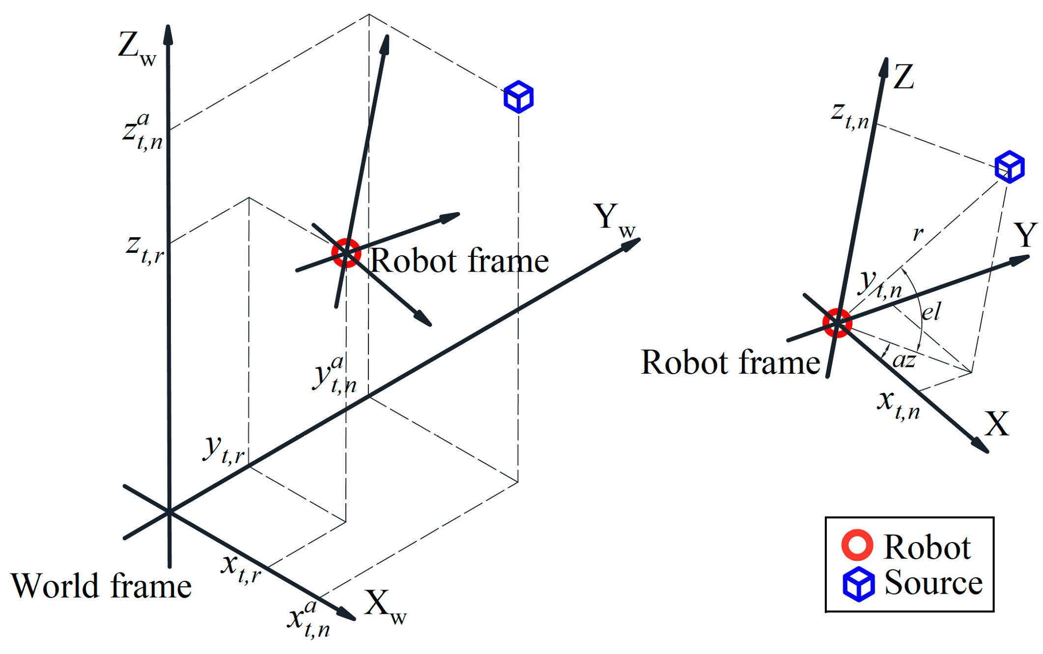
2. Problem Formulation

In previous acoustic SLAM research, the applied robot movement model always constrained the robot’s velocity to be along the direction of orientation of the robot [5,6,7]. This constraint can be easily satisfied in simulation. Meanwhile, the coupling of the robot’s orientation and its velocity direction simplified the mathematical deduction. However, it is only practical in a few kinds of real robots, for instance, two-wheel robots.

For the sake of generality, a three-dimensional robot movement model is applied in the proposed method. The model decouples the direction of the robot’s velocity from its orientation; thus, it is suitable for most real robots, such as drones. As depicted in Figure 1, the robot’s state at time t is considered as ${\mathbf{r}}_t$= [${\mathbf{p}}_t^T$, ${\mathbf{R}}_t$], where ${\mathbf{p}}_t$= [u_x,t,r, u_y,t,r, u_z,t,r, v_x,t,r, v_y,t,r, v_z,t,r] is the position/velocity vector and ${\mathbf{R}}_t$ is the rotation matrix corresponding to the robot’s orientation. Symbols az, el, and r in Figure 1 denote the azimuth, elevation, and radius of the sound source in the robot frame, respectively. The robot dynamics are given by:

$${\mathbf{p}}_t={\mathbf{F}}_t{\mathbf{p}}_{t-1}+d{\mathbf{p}}_{t-1|t}+{\mathbf{v}}_{t,\mathbf{p}},\hspace{1em}{\mathbf{v}}_{t,\mathbf{p}} \sim \mathcal{N}({\mathbf{0}}_{\mathbf{6}\times \mathbf{1}},{\mathbf{\Sigma }}_{t,\mathbf{p}})$$

(1)

$${\mathbf{R}}_t=\zeta ({[\theta ,\psi ,\phi ]}^T+{\mathbf{v}}_{t,\mathbf{R}}),\hspace{1em}{\mathbf{v}}_{t,\mathbf{R}} \sim \mathcal{N}({\mathbf{0}}_{\mathbf{3}\times \mathbf{1}},{\mathbf{\Sigma }}_{t,\mathbf{R}})$$

(2)

where ${\mathbf{v}}_{t,\mathbf{p}}$ denotes unbiased Gaussian noise with covariance ${\mathbf{\Sigma }}_{t,\mathbf{p}}$. dp_t−1|t is the small variation of ${\mathbf{p}}_t$ from time step t − 1 to t, and ζ(θ, ψ, φ) is a nonlinear function converting Euler angles, [θ, ψ, φ], to a rotation matrix. The matrix F_t and dp_t−1|t are given by:

$${\mathbf{F}}_t=[ I_6 ]$$

(3)

$$d{\mathbf{p}}_{t-1|\mathrm{t}}=[d{u}_{x,t-1|t},d{u}_{y,t-1|t},d{u}_{z,t-1|t},d{v}_{x,t-1|t},d{v}_{y,t-1|t},d{v}_{z,t-1|t}]$$

(4)

where I_n is the n×n identity matrix. It is clear that du_x,t−1|t, du_y,t−1|t, and du_z,t−1|t are related to dv_x,t−1|t, dv_y,t−1|t, and dv_z,t−1|t. The method to estimate these values will be introduced in Section 3.

The measurements of the robot velocity v and orientation R are defined as y_t≜[$y_{t,v}$, $y_{t,\mathbf{R}}$] and modeled as:

$$y_{t,\mathit{v}}=h{\mathbf{p}}_t+{\mathbf{w}}_{t,\mathit{v}}$$

(5)

$$y_{t,\mathbf{R}}=\zeta ({[\theta ,\psi ,\phi ]}^T+{\mathbf{w}}_{t,\mathbf{R}})\hspace{1em}, {\mathbf{w}}_{t,\mathbf{R}} \sim \mathcal{N}({\mathbf{0}}_{3\times 1},{\mathsf{\sigma }}_{\mathbf{w},{\mathbf{R}}_t}^2)$$

(6)

where ${\mathbf{w}}_{t,v}$ is non-Gaussian noise, and ${\mathbf{w}}_{t,\mathbf{R}}$ denotes the measurement of Gaussian noise with covariance ${\mathsf{\sigma }}_{\mathbf{w},{\mathbf{R}}_t}^{\mathbf{2}}$. In addition, h≜[0_{3 × 3}, I₃]. In fact, robots equipped with a 9-axis IMU can provide accurate Euler angles with small errors. Therefore, D-D SLAM neglects the influence of the measurement noise on orientation, which means that ${\mathsf{\sigma }}_{\mathbf{w},{\mathbf{R}}_t}^2$ is considered to be zero. Thus, (6) can be simplified to:

$$y_{t,R}=y_{t-1,R}\mathbf{\Delta }{R}_{t-1|t}$$

(7)

where ΔR_t−1|t denotes the constraints of robot orientation from time step t − 1 to t and is introduced in Section 3.

As the absolute positional state of the sound source is the landmark in mapping, the absolute state (${\mathrm{s}}_{t,n}^a$≜[$x_{t,n}^a$, $y_{t,n}^a$, $z_{t,n}^a$]^T) of source n in the world frame at time step t is defined as [7]:

$${\mathrm{s}}_{t,n}^a={\mathrm{s}}_{t-1,n}^a+{\mathbf{n}}_{t,n},\hspace{1em}\hspace{1em}{\mathbf{n}}_{t,n} \sim \mathcal{N}({\mathbf{0}}_{3\times 3},\mathbf{Q})$$

(8)

where n = 1,…,$N_t$ is the index of $N_t$ sources, the superscript a stands for the world frame, and ${\mathbf{n}}_{t,n}$ is the process noise with covariance Q. The transformation of the source’s position in the world frame to that in the robot frame is given by:

$${\mathrm{s}}_{t,n}=\mathbf{\Gamma }({\mathrm{s}}_{t,n}^a-{[u_{x,t,r}^{},u_{y,t,r}^{},u_{z,t,r}^{}]}^T),\hspace{1em}\mathbf{\Gamma }={\mathbf{R}}_t$$

(9)

where ${\mathrm{s}}_{t,n}$≜[$x_{t,n}$, $y_{t,n}$, $z_{t,n}$]^T is the positional state of the source in the robot frame, and Γ is the rotation matrix between the world frame and the robot frame.

The bearing information of the source is estimated by the DoA algorithm and is modeled as [7]:

$${\mathsf{\Omega }}_t=[{\displaystyle \underset{n=1}{\overset{Nt}{\cup }}D({\mathrm{s}}_{t,n})}]\cup K_t$$

(10)

where D(${\mathrm{s}}_{t,n}$) is the process that models the missing DoAs and estimation errors, and $K_t$ denotes the Poisson point process of $N_t$ independent and identically distributed (IID) false DoA estimates distributed uniformly over a unit sphere.

The source’s distance from the sensors is also estimated solely with the DRR. The DRR estimation method is developed using interaural magnitude-squared coherence (MSC), and the source’s distance is estimated by computing the discrete Fourier transform (DFT) on overlapped windowed signal frames [16]. A small sound piece is sampled at time step t and divided into several parts by a sliding window. In each part of the sound piece, the source’s distance from the sensors is estimated. The estimation is modeled by:

$${\widehat{d}}_{t,\mu }^n\sim \mathcal{N}(d_t^n,R_{t,d})$$

(11)

where μ denotes the windowed signal frame indices, and $d_t^n$ is the true source’s distance from the sensors at time step t. In a short time, the estimated distances ${\widehat{d}}_{t,\mu }^n$ in different window frames at time step t tend to follow a nearly normal distribution that is modeled with the mean $d_t^n$ and the covariance $R_{t,d}$.

The positional state of the sources in the robot frame ${\mathrm{s}}_{t,n}$ is associated with the DoA, and the distances of the sources are computed with the DRR. The relationship is as follows:

$$\left\{\begin{array}{c}{[{\mathsf{\omega }}_{t,m},r_{t,m}]}^T=\mathcal{G}\left({\mathrm{s}}_{t,n}\right)+{\mathbf{e}}_{t,m}\\ {\mathbf{e}}_{t,m}\sim \mathcal{N}({\mathbf{0}}_{3\times 1},diag(R_{t,\mathrm{m}},R_{t,\mathrm{d}}))\end{array}\right.$$

(12)

where m = 1,…,M_t denotes the index of DoA estimates, M_t is the number of DoA estimates in time step t, ω_t,m = [${\varphi }_{t,m}$, ${\gamma }_{t,m}$]^T, $\mathcal{G}$(•) is a function that is used to transform from Cartesian coordinates to spherical coordinates (azimuth ${\varphi }_{t,m}$, elevation ${\gamma }_{t,m}$, and radius $r_{t,m}$), and ${\mathbf{e}}_{t,m}$ denotes the measurement error with covariance which consists of DoA estimation covariance $R_{t,m}$ and distance estimation covariance $R_{t,d}$.

Estimating r_t and ${\mathrm{s}}_{t,n}^a$ using Ω_t, ${\widehat{d}}_{t,\mu }^n$, and y_t, presents more challenges than other methods.

(1)

The robot’s movement is nonuniform motion, and the velocity direction is decoupled from the robot’s orientation. Therefore, the robot dynamics in this paper have more freedom of motion than in [5,6,7], meaning the movement estimation becomes more complex and difficult.

(2)

The velocity and orientation are measured using an IMU, whose velocity measurement noise is non-Gaussian and nonlinear. This kind of noise is common in real instruments and cannot be simply removed with a traditional Kalman filter or even an extended Kalman filter (EKF) by fusing DoA measurements due to its strong nonlinearity.

(3)

The distance estimation and the DoA measurement usually intermingle with strong noise and disturbances, causing a few incorrect estimations of the sound source position, leading to no convergence.

(4)

The critical distance, which is essential for the estimation of the distance from the DRR, is usually calculated with the acoustic coefficients and geometry of the room. However, these parameters are unknown in our situation.

As mentioned before, new constraints, i.e., the source’s distance from the sensor, are needed to overcome challenges 1 and 2. Based on a particle algorithm, a method for online estimation of the critical distance is designed to handle challenge 4, which will be introduced in Section 4. Regarding challenge 3, a filter based on a Gaussian mixture model is implemented, which will be discussed in Section 4.

3. Background Knowledge about IMU Preintegration and DRR

3.1. IMU Preintegration

To summarize hundreds of inertial measurements into a single relative motion constraint and update the robot states expediently, IMU preintegration [17] is used in this paper. The absolute robot state is updated by [17]:

$$R_t=R_{t-1}\mathbf{\Delta }{R}_{t-1|t}$$

(13)

$$V_t=V_{t-1}+g\Delta t+R_t\Delta V_{t-1|t}$$

(14)

$$X_t=X_{t-1}+V_{t-1}\Delta t+\frac{1}{2}g\Delta t^2+R_t\Delta X_{t|t-1}$$

(15)

where X_t = [u_x,t,r, u_y,t,r, u_z,t,r]^T, V_t = [$v_{x,t,r}$, $v_{y,t,r}$, $v_{z,t,r}$]^T, g denotes the gravitational acceleration, Δt is the time difference from time step t − 1 to t, and ΔR_t−1|t, ΔX_t|t−1, and ΔV_t|t−1 represent the pre-integrated measurements calculated with Gaussian pre-integrated measurements (GPMs) [18]. To be specific, ΔR_t−1|t, ΔX_t|t−1, and ΔV_t|t−1 are estimated with Equations (20), (27), and (26) of Ref. [18], respectively, by feeding IMU measurements.

3.2. DRR Computing and Distance Estimator

For distance estimation, it is useful to determine how sound is reflected in reverberant fields. The DRR is a useful ratio to estimate a source’s distance [19] and can be calculated using only acoustic data. The source’s distance d(μ) is estimated by

$$d(\mu )=d_c{(\sqrt{{\eta }_{\mathrm{MSC}}(\mu )})}^{-1}$$

(16)

where η_MSC(μ) is the broadband DRR calculated with the algorithm based on interaural MSC [16], and d_c is the critical distance that connects the source’s distance and the DRR. The equivalent relative HRTF of the microphone array is used to apply the MSC [16] on drone data. The interaural level difference is estimated with the directivity indices of the microphone array, and the interaural time difference (ITD) is calculated with the DoA result and the array shape. The coherence of the reverberant components is set as a sinc function related to the frequency index and the pairwise distance between microphones [20]. The d_c is defined as [19]:

$$d_c=0.1\sqrt{{\rho }_s{\rho }_r}\sqrt{V_R{(\pi T_{60})}^{-1}}$$

(17)

The accuracy of the proposed D-D SLAM is based on the source’s distance estimation with the DRR. A large reverberation time, which indicates a small critical distance, contributes to the improvement of the source’s distance estimation with the DRR, but larger reverberation times also make the estimation of ITD and ILD more distorted, which may affect the DRR estimation [16]. If the critical distance is too small, the reverberant energy received by the microphone array is much larger than the direct energy, and thus, the ITD and ILD would be seriously affected. If the critical distance is too large, the direct energy received by the microphone array is much larger than the reverberant energy, so the acoustical field of the room is similar to the free field. The acoustical free field does not meet the subject of the proposed D-D SLAM. Thus, the D-D SLAM cannot be used outdoors.

For common SLAM problems, the critical distance d_c is initially unknown because the source directivity indices ρ_s, the receiver directivity indices ρ_r, the room volume V_R and the reverberation time T₆₀ cannot be measured in advance. Hence, an online method is proposed in Section 4 to estimate the critical distance during SLAM exploration.

4. Mapping and Locating

With the fundamental theory of SLAM [21], the acoustic SLAM problem can be modeled with the SLAM posterior probability density function (PDF), which is usually factorized into two parts:

$$p(r_t,s_t,d_c|{\mathsf{\eta }}_{1:t},{\mathsf{\Omega }}_{1:t},y_{1:t})=p(s_t|r_t,{\mathsf{\Omega }}_{1:t})p(r_t,d_c|{\mathsf{\eta }}_{1:t},{\mathsf{\Omega }}_{1:t},y_{1:t})$$

(18)

where s_t is the set of all sound source positions, p(s_t | r_t, Ω_1:t) is a sound source’s position posterior PDF corresponding to the mapping problem in SLAM, and p(r_t, d_c |η_1:t, Ω_1:t, y_1:t) represents the robot posterior PDF corresponding to the locating problem in SLAM. The critical distance d_c is the random variable to be estimated. η_1:t denotes the DRR estimates from the beginning to time step t that are computed with the method based on interaural MSC [16].

4.1. Mapping

The sound sources are considered landmarks on the map, so the focus of the mapping procedure is the estimation of the source positions. To solve existing problems, including false DoA estimates, Evers et al. [7] proposed a mapping method based on probabilistic source triangulation and a random finite set. Their method performs well when the robot keeps moving and receiving a signal from the sound source. However, when the positions of both the robot and the sound source remain stationary, mapping mistakes may occur during the emerging process, which is often used to limit the number of Gaussian mixture (GM) components. In this situation, the robot’s position and DoA estimates do not change, resulting in the repeated emergence of the same new GM components located in the same zone. As the new GM components satisfy both the wrapped Gaussian distribution in angle and the uniform distribution in the radial direction [7], the component’s distribution density in the sector region is uneven. The distance between any two GM components l can be calculated by:

$$l=\sqrt{2r^2+\Delta r^2+2r\Delta r(1-\cos (\Delta \gamma ))}$$

(19)

where r is one of the component’s distances from the robot, and Δr and Δγ are the difference between the two components in radius and angle, respectively. With the same Δr and Δγ, the shorter the radius distance of the GM component is, the shorter the distance between different GM components is. Thus, the component density in the region closer to the robot is higher than others. Figure 2c reveals this false trend.

Before the clustering of GM components for source estimation, mixture reduction is usually applied to limit the number of components through merging. The criterion equation of merging components is given by [22]:

$${(m_k^i-m_k^j)}^T{(P_k^i)}^{-1}(m_k^i-m_k^j)\le U,\hspace{1em}i=1,\dots ,J_k$$

(20)

where J_k is the number of GM components, j is the index of the component with the maximum weight, $m_k^i$ denotes the position of the GM component in the robot frame, $P_k^i$ is the covariance of the GM component’s position, and U is the threshold of merging.

With the criterion Equation (20), it is found that the component merging is relevant to the covariance and the range between components. The new components are created with the same covariance and weight. Therefore, when they have a denser distribution (closer to the robot), they are more likely to be merged together, forming merged components with larger weights. When both the sound source and the robot remain stationary, new components will be created repeatedly in the same zone, and the distribution of weights (after merging) will become increasingly uneven over time. The area closer to the robot will receive much larger weights compared with that far from the robot. This trend has a negative influence on GM component clustering and may finally lead to a false estimation of the sound source position, indicating that it is much closer than the true value. Here, a simulation test is conducted to illustrate the problem mentioned above, while a solution will also be introduced in this section. The simulation test setup is basically the same as that of part C in Section 4 of [7], while an extra time segment is added when the robot remains stationary for several time steps.

Figure 2 is a heatmap of the source weight density calculated using the origin method [7] in the simulation setup with an extra time segment. A higher saturation level of red indicates a higher weight density. As shown in Figure 2a, just after the robot moved for three time steps (same as that in the original simulation [7]), the GM components were clustered into the place close to the true source where the probability density peak is located. However, as shown in Figure 2b,c, the longer the robot remains stationary, the greater the peak of the probability density deviates toward the robot. The same trend can be found with the weighted centroid of the GM components. This deviation causes an incorrect estimation of the source position, leading to incorrect mapping.

To fix this problem, a solution is developed. The solution is the use of keyframes. When the robot and source remain stationary, new GM components are always created in the same region so that the new GM components are merged into a false component with a large weight. The weight of the false component increases over time, and the weighted centroid of the components is eventually shifted toward the robot. If the creation and merging of GM components stop when the robot and source remain stationary, a false component with a large weight is avoided. The basic idea is that a keyframe factor is calculated to evaluate the difference between the current frame and the last keyframe:

$$T=({\widehat{T}}_t^1>T_{KF}^1)\Vert ({\widehat{T}}_t^2>T_{KF}^2)\Vert ({\widehat{T}}_t^3>T_{KF}^3)$$

(21)

$$\left\{\begin{array}{l}{\widehat{T}}_t^1=\Vert {(u_{x,t,r},u_{y,t,r},u_{z,t,r})}^T-{(u_{x,KF,r},u_{y,KF,r},u_{z,KF,r})}^T\Vert \hfill \\ {\widehat{T}}_t^2=\mathrm{OSPA}({\mathsf{\Omega }}_t,{\mathsf{\Omega }}_{KF})\hfill \\ {\widehat{T}}_t^3=\Vert {\zeta }^{-1}(R_t{R}_{KF}^T)\Vert \hfill \end{array}\right.$$

(22)

where the subscript KF denotes a keyframe, $T_{KF}^k$ for k = 1, 2, 3 denotes the given threshold of the keyframe, ||•|| is the two-norm, ζ⁻¹(•) is a function converting a rotation matrix to Euler angles, || indicates the OR operation, and OSPA is the Optimal Subpattern Assignment distance [23]. The correspondence of the DOA estimations between the two sets is unknown, so the OSPA is applied for the best match. The OSPA is defined as:

$$\mathrm{OSPA}({\mathsf{\Omega }}_t,{\mathsf{\Omega }}_{KF})=[\frac{1}{N}\underset{\pi \in {\mathsf{\Pi }}_N}{\min }{\displaystyle \sum _{i=1}^M{l}_c({\Omega }_{t,i},{\Omega }_{KF,\pi (i)})+(N-M)c}]$$

(23)

where Ω_t≜{Ω_t,1,…, Ω_t,N}, Ω_KF≜{Ω_KF,1,…, Ω_KF,M}, Π_N stands for the set of permutations of length M with elements from {1, …, N}, l_c (Ω_t,i, Ω_KF,π(i)) = min(c, || Ω_t,i − Ω_KF,π(i)||) and c is a cutoff value of 30°.

When the robot and the source remain stationary, ${\widehat{T}}_t^k$ will be less than $T_{\mathit{KF}}^k$, making T false. When T is false, the current frame in time step t is not a keyframe. In contrast, when the robot moves far enough, ${\widehat{T}}_t^k$ becomes larger than $T_{\mathit{KF}}^k$, making T true. Thus, the current frame is considered a new keyframe, and the state of the keyframe is updated with the following equations:

$$\left\{\begin{array}{l}{(u_{x,KF,r},u_{y,KF,r},u_{z,KF,r})}^T={(u_{x,t,r},u_{y,t,r},u_{z,t,r})}^T\hfill \\ {\mathsf{\Omega }}_{KF}={\mathsf{\Omega }}_t\hfill \\ R_{KF}^{}=R_t\hfill \end{array}\right.$$

(24)

When GM components are only created and merged in keyframes, a false merged component with a large weight is avoided. To eliminate accidental errors, a limiting filter is applied to the clustering of GM components. The limiting filter is modeled as:

$$\mathrm{LF}({\mathrm{s}}_t)=\left\{\begin{array}{cc}{\mathrm{s}}_t ,\hfill & \hspace{1em}\mathrm{OSAP}({\mathrm{s}}_t,{\mathrm{s}}_{t-1})\le s_{LF}\hfill \\ {\mathrm{s}}_{t-1},\hfill & \hspace{1em}\mathrm{OSAP}({\mathrm{s}}_t,{\mathrm{s}}_{t-1})>s_{LF}\hfill \end{array}\right.$$

(25)

where s_t is the source estimation which is calculated with the mapping method based on probabilistic source triangulation and random finite set [7] by feeding the data of keyframe, $s_{LF}$ denotes the threshold value of the limiting filter, which is related to the maximal variation of the source position between time steps t − 1 and t. The OSAP is also applied, but the cutoff value c is changed to 0.5 m.

Using the probabilistic source triangulation in [7] and the keyframe method mentioned above, the source posterior PDF p(s_t | r_t, Ω_1:t) can be estimated using the evidence of the DoA estimation $\mathcal{L}$(Ω_t | r_t, d_c). The implementation is given by:

$$\mathcal{L}\left({\mathsf{\Omega }}_t|r_t,d_c\right)\triangleq e^{-N_{t,c}-p_d{N}_{t|t-1}}{\displaystyle \prod _{m=1}^{M_t}}\mathcal{l}\left({\mathsf{\omega }}_{t,m}|r_t,d_c\right)$$

(26)

where p_d denotes the probability of detection, N_t,c is the number of false alarms, N_t|t−1 stands for the quantity of predicted features [7], and ${\mathsf{\omega }}_{t,m}$ is the DoA estimation computed from the GM components and the position of the robot. ℓ(${\mathsf{\omega }}_{t,m}$|r_t,d_c) is evaluated with Equation (34) in [7]. The mapping process is only fed with the data of the keyframe.

4.2. Locating

This section proposes a method to estimate the robot’s location by fusing the IMU measurements and the DoA and DRR estimates. Additionally, the critical distance is estimated online. Because the relationship between the state of the robot and the sensor measurements is nonlinear and complicated, it is difficult to estimate the critical distance d_c and the state of the robot ${\mathbf{r}}_t$ directly from just the IMU measurements and the DoA and DRR estimates. Particle filters [24] are usually applied to model the robot posterior PDF of this nonlinear problem. With this method, the robot posterior PDF p(r_t, d_c |η_1:t, Ω_1:t, y_1:t) is modeled as:

$$p(r_t,d_c|{\mathsf{\eta }}_{1:t},{\mathsf{\Omega }}_{1:t},y_{1:t})\approx {\displaystyle \sum _{i=1}^I{\mathsf{\alpha }}_t^i{\mathsf{\delta }}_{{\widehat{\mathbf{r}}}_t^i,{\widehat{d}}_c^i}}({\mathbf{r}}_t,d_c)$$

(27)

where I is the number of particles, ${\mathsf{\alpha }}_t^i$ denotes the weight of a particle, and ${\delta }_{{\widehat{r}}_t^i,{\widehat{d}}_c^i}$ (${\mathbf{r}}_t$, $d_c$) is the Dirac-delta function centered at ${\mathbf{r}}_t$, $d_c$ and evaluated at ${\widehat{\mathbf{r}}}_t^i$, ${\widehat{d}}_c^i$. Because the state of the robot and the critical distance are estimated at the same time, there is a large amount of uncertainty, so large quantities of particles are required to model the robot posterior PDF.

Using (16) the source’s distance from robot $\widehat{d}$ can be computed with the DRR if the critical distance is known. As the source’s distance is helpful in the estimation of the robot’s position, it is easier to estimate the state of the robot when the critical distance is known. To simplify the robot posterior PDF, the marginalization [25] is adopted to decouple the posterior PDF into that of $d_c$ and ${\mathbf{r}}_t$ separately, i.e., the robot posterior PDF p(r_t, d_c |η_1:t, Ω_1:t, y_1:t) is factorized into two parts:

$$p(r_t,d_c|{\mathsf{\eta }}_{1:t},{\mathsf{\Omega }}_{1:t},y_{1:t})=p(d_c|{\mathsf{\eta }}_{1:t},{\mathsf{\Omega }}_{1:t},y_{1:t})p(r_t|d_c,{\mathsf{\eta }}_{1:t},{\mathsf{\Omega }}_{1:t},y_{1:t})$$

(28)

Using (15), the state of the robot can be computed from the IMU measures. Meanwhile, the source’s distance from the robot computed from a given d_c, η_1:t using (16), and DoA estimates can be used to correct the state of the robot. Therefore, this paper takes the estimation of the robot’s state r_t as a nonlinear substructure [25] of the estimation of critical distance d_c. Thus, for each d_c particle, there is a substructure corresponding to the robot state and the source position.

The critical distance is assumed to be within a certain range ${\widehat{d}}_c$∈[$d_c^{min}$, $d_c^{max}$] and obeys a uniform distribution:

$${\widehat{d}}_c^i\sim \mathcal{U}(d_c^{min},d_c^{max}),\hspace{1em}\hspace{1em}\hspace{1em}i=1,\dots ,I$$

(29)

where $d_c^{min}$ and $d_c^{max}$ are the minimum and maximum of the critical distance, respectively, and I is the number of particles. A critical distance particle is drawn from the uniform distribution. For each critical distance particle and each source, the estimations of the source’s distance at time step t can be calculated in the following formula according to (16):

$${\widehat{d}}_{t,m,\mu }^i={\widehat{d}}_c^i{(\sqrt{{\eta }_{t,m,\mu }})}^{-1},\hspace{1em}\hspace{1em}\mu =1,\dots ,B$$

(30)

where B denotes the number of windowed signal frames in time step t, m = 1, …, M_t and ${\widehat{d}}_{t,m,\mu }^i$ is the source’s distance corresponding to ${\widehat{d}}_c^i$.

Theoretically, the state of the robot can be computed using iterative calculation of (13)–(15) as long as the initial value of the robot’s state is given. In fact, a 9-axis acceleration gyroscope sensor can provide an accurate rotation matrix ${\mathbf{R}}_t$ that can be used to accurately describe the attitude of the robot. Therefore, ${\mathbf{R}}_t$ is computed directly from IMU measurements and the GPMs in this paper. However, the velocity and position of the robot cannot be computed using only the IMU measurements due to unacceptable integral error. Therefore, the DoA estimates and DRR are used to eliminate those errors by fusing all measures with an EKF [26]. For weakly nonlinear systems, an EKF has better performance than a Kalman filter. The sound source distance estimation from DRR is added as a constraint to suppress the noise of IMU measurements along the direction of sound arrival. With the addition of range information, the state of the robot has weaker nonlinearity than that of the robot which only contains bearing information and IMU measurements. Therefore, EKF is suitable for the estimation of the weakly nonlinear state of the robot in D-D SLAM. Using (13)–(15), the implementation of the EKF is given by:

$$X_t^{\prime i}=X_{t-1}^i+V_{t-1}^i\Delta t+\frac{1}{2}g\Delta t^2+R_t{}_{}\Delta X_{t-1|t}$$

(31)

where $X_t^{\prime i}$ denotes the prediction of the robot’s position in the EKF. The rotation matrix ${\mathbf{R}}_t$ and the velocity V_t are determined from Equations (13) and (14). The pre-integrated measurement of position ΔX_t−1|t is estimated with Equation (27) of Ref. [18] by feeding IMU measurements. The prediction of covariance in the EKF is given by:

$${Cov}_{t,m}^{\prime i}=F_{t}Co{v}_{t-1,m}^i{F}_t{}^T+Q_{X_t}^i$$

(32)

where ${Cov}_{t-\mathit{1},m}^i$ denotes the covariance of the EKF, ${\mathbf{F}}_t$ is given by (3) and $Q_{X_t}^i$ is the process non-Gaussian noise of the robot position. ${\mathbf{Q}}_{X_t}^i$ is associated with the process noise of the robot’s velocity, according to (31) with the variance-covariance propagation law:

$$Q_{V_t}^i=Q_{V_{t-1}}^i+d{Q}_{V_{t-1|t}}$$

(33)

$$Q_{X_t}^i=Q_{X_{t-1}}^i+\Delta t_{}{Q}_{V_{t-1}}^i\Delta t+d{Q}_{X_{t-1|t}}$$

(34)

where d$Q_{X_{t-1|t}}$ and d$Q_{V_{t-1|t}}$ denote the variances of the GPMs of the robot’s position and velocity, respectively. For each source, the observational equation in the EKF is determined by:

$${[{\widehat{\mathsf{\omega }}}_{t,\mathrm{m}}^i,{\widehat{r}}_{t,\mathrm{m}}^i]}^T=\mathcal{G}({\mathbf{R}}_t(X_t^{\prime i}-{\widehat{\mathrm{s}}}_{t-1,m}^i))$$

(35)

where m = 1, …, M_t, R_t is estimated with Equation (13) and $\mathcal{G}$(•) is the Cartesian-to-spherical transformation. According to the mapping procedure (Section 4.1), the estimation of source ${\widehat{\mathrm{s}}}_{t-\mathit{1},m}^i$ is given using GM component clustering of the keyframe data. Hence, the Kalman gain and the correction of Kalman gain are given by:

$$K_{t,m}^i=Co{v}^{\prime }{{}_{t,m}^i}_{}{(H_{t,m}^i)}^T{}_{}{(H_{t,m}^i{}_{}Co{v}^{\prime }{{}_{t,m}^i}_{}{(H_{t,m}^i)}^T+R_{EKF})}^{-1}$$

(36)

$${\widehat{X}}_{t,m,\mu }^i=X^{\prime }{}_t^i+K_{t,m}^i({[{\mathsf{\Omega }}_{t,m},{\widehat{d}}_{t,m,\mu }^i]}^T-{[{\widehat{\mathsf{\omega }}}_{t,\mathrm{m}}^i,{\widehat{r}}_{t,\mathrm{m}}^i]}^T)$$

(37)

$${\widehat{V}}_{t,m,\mu }^i=({\widehat{X}}_{t,m,\mu }^i-X_{t-1}^i)/dt$$

(38)

$$Co{v}_{t,m}^i=(I_3-K_{t,m}^i{}_{}{H}_{t,m}^i)Co{v}^{\prime }{}_{t,m}^i$$

(39)

where H is the Jacobian matrix of the observational equation, ${\widehat{V}}_{t,m,\mu }^i$ is the velocity of the robot corresponding to each output of the EKF, dt denotes the time difference between two adjacent keyframes, which is different from Δt, and ${\mathbf{R}}_{EKF}$ is the measurement noise, which is assumed to be known. The output of the EKF, ${\widehat{X}}_{t,m,\mu }^i$, corresponds to each source’s distance ${\widehat{d}}_{t,m,\mu }^i$. As the estimation of the robot’s position is nonlinear and the rotation matrix R_t is computed directly from IMU measurements, the Gaussian mixture model (GMM) is applied to model the robot posterior PDF p(X_t |d i c, η_1:t, Ω_1:t, y_1:t):

$$p(X_t|d_c^i,{\mathsf{\eta }}_{1:t},{\mathsf{\Omega }}_{1:t},y_{1:t})={\displaystyle \sum _{M_t}^m{\displaystyle \sum _{\mathrm{B}}^{\mu }{w}_{t,m,\mu }^i{}_{}}\mathcal{N}(X_t|{\widehat{X}}_{t,m,\mu }^i,Co{v}_{t,m}^i)}$$

(40)

where $w_{t,m,\mu }^i$ denotes the weights of the GM components in the windowed signal frame indices μ of time step t and is given by:

$$w_{t,m,\mu }^i=\mathcal{N}({\widehat{X}}_{t,m,\mu }^i|X^{\prime }{}_t^i,Q_{X_t}^i)$$

(41)

It is clear that the smaller the difference between the outputs of the EKF and GPMs is, the larger the component weight $w_{t,m,\mu }^i$ is. For the GMM, the estimation of the robot position, the robot velocity, the source’s distance from the robot, and the covariance in the EKF are computed with the weighted average method

$$X_t^i={\displaystyle \sum _{M_t}^m{\displaystyle \sum _B^{\mu }{w}_{t,m,\mu }^i{}_{}{\widehat{X}}_{t,m,\mu }^i}}$$

(42)

$$V_t^i={\displaystyle \sum _{M_t}^m{\displaystyle \sum _B^{\mu }{w}_{t,m,\mu }^i{}_{}{\widehat{V}}_{t,m,\mu }^i}}$$

(43)

$$d_{t,m}^i=\Vert X_t^i-{\widehat{\mathrm{s}}}_{t,m}\Vert$$

(44)

$$Co{v}_{t,m}={\displaystyle \sum _{M_t}^m{\displaystyle \sum _B^{\mu }{w}_{t,m,\mu }^i{}_{}Co{v}_{t,\mu }^i}}$$

(45)

The weight of each critical distance and robot position particle is given by:

$${\alpha }_t^i=\mathcal{N}(X_t^i|X^{\prime }{}_t^i,Q_{X_t}^i)$$

(46)

Equation (46) reflects the coincidence degree between the robot position corresponding to each critical distance particle and the GPM measurements. The GPMs of the IMU are used to evaluate each critical distance particle. The weights of the critical distance particle that fits the GPM measurements well will become larger. The final estimation of the robot and source position will be in the best interests of all measurements.

4.3. Posterior PDF of the D-D SLAM

This section provides the implementation of evaluating the SLAM posterior PDF. Because a rotation matrix can describe the attitude of the robot accurately with the GPMs of the IMU data and the source triangulation does not depend on velocity, (18) is reduced to:

$$p(X_t,s_t,d_c|{\mathsf{\eta }}_{1:t},{\mathsf{\Omega }}_{1:t},y_{1:t})=p(s_t|X_t,{\mathsf{\Omega }}_{1:t})p(X_t,d_c|{\mathsf{\eta }}_{1:t},{\mathsf{\Omega }}_{1:t},y_{1:t})$$

(47)

According to the Bayes rule, using (26) and (27), the posterior PDF p(X_t, d_c |η_1:t, Ω_1:t, y_1:t) is given by:

$$p(X_t,d_c|{\mathsf{\eta }}_{1:t},{\mathsf{\Omega }}_{1:t},y_{1:t})=\frac{{\displaystyle \sum _{i=1}^I{\alpha }_t^i{}_{} \mathcal{L}{\left({\mathsf{\Omega }}_t|{\widehat{X}}_t,{\widehat{d}}_c\right)}_{}{\mathsf{\delta }}_{{\widehat{X}}_t,{\widehat{d}}_c^i}(X_t,d_c)}}{{\displaystyle \sum _{j=1}^I{\alpha }_t^j{}_{} \mathcal{L}\left({\mathsf{\Omega }}_t|{\widehat{X}}_t,{\widehat{d}}_c\right)}}$$

(48)

Using (48) in (47), the SLAM posterior PDF is reduced to:

$$p(X_t,s_t,d_c|{\mathsf{\eta }}_{1:t},{\mathsf{\Omega }}_{1:t},y_{1:t})={{\displaystyle \sum _{i=1}^I{\beta }_t^i {}_{}{\mathsf{\delta }}_{{\widehat{X}}_t,{\widehat{d}}_c^i}(X_t,d_c)}}_{} p(s_t|X_t,{\mathsf{\Omega }}_{1:t})$$

(49)

$${\beta }_t^i=\frac{{\alpha }_t^i{}_{} \mathcal{L}\left({\mathsf{\Omega }}_t|{\widehat{X}}_t,{\widehat{d}}_c\right)}{{\displaystyle \sum _{j=1}^I{\alpha }_t^j{}_{} \mathcal{L}\left({\mathsf{\Omega }}_t|{\widehat{X}}_t,{\widehat{d}}_c\right)}}$$

(50)

where ${\beta }_t^i$ is the weight and is used to evaluate the particle and estimate the position of the robot and the source. The D-D SLAM is summarized in pseudocode (see Algorithm 1).

Algorithm 1: D-D SLAM
Data: DoAs Ωt, DRR ηt, IMU Measure yt
for i = 1, …, I do
		Compute ${\widehat{\mathbf{r}}}_t^i$ using (13)(14)(15);
		Compute KeyFrame factor using (21)(22);
		if KeyFrame then
				Compute ${\mathrm{Q}}_{X_t}^i$, $\mathrm{C}\mathrm{o}{\mathrm{v}}^{\prime }{{}_{t,m}^i}_{}$ using (34)(33)(32);
				for m = 1, …, Mt do
						Predict ${\widehat{\mathsf{\omega }}}_{t,m}^i$, ${\widehat{r}}_{t,m}^i$ using (35);
						Compute ${\mathbf{K}}_{t,m}^i$ using (36);
						for µ = 1, …, B do
								Evaluate ${\widehat{\mathbf{X}}}_{t,m,\mu }^i$, ${\widehat{\mathbf{V}}}_{t,m,\mu }^i$ using (37)(38);
								Compute $w_{t,m,\mu }^i$ using (41);
						end
				end
				Update Covt,m using (45);
				Update ${\mathbf{X}}_t^i$, ${\mathbf{V}}_t^i$ using (42)(43);
				Evaluate ${\mathsf{\alpha }}_t^i$ using (46);
				Compute ${\mathrm{s}}_t^i$ using the mapping method [7] by  feeding the date of keyframe;
				GM reduction of mapping [27];
				Evaluate $\mathcal{L}$(Ωt | rt, dc) using (26);
				Evaluate ${\beta }_t^i$ using (50);
				Update particle state;
		else
				Update ${\mathrm{Q}}_{X_t}^i$, $\mathrm{C}\mathrm{o}{\mathrm{v}}^{\prime }{{}_{t,m}^i}_{}$ using (34)(33)(32);
		end
end
Resampling [28];

Each particle is now evaluated by the evidence of mapping (26) and the weight of locating (46). When the velocity of the robot is updated with (43), first-order recursive temporal smoothing is applied to smooth the speed to minimize the jitter of the velocity:

$$V_t^i=a_p{}_{}{V}_{t-1}^{\mathrm{i}}+(1-a_p){\displaystyle \sum _{M_t}^m{\displaystyle \sum _B^{\mu }{w}_{t,m,\mu }^i{}_{}{\widehat{V}}_{t,m,\mu }^i}}$$

(51)

where a_p is a smoothing parameter. In the procedure “Update particle state”, the estimation of the robot and the source at time step t is computed with the weighted mean method.

5. Simulation and Experiment Setup

5.1. Simulation Setup

This simulation is designed to compare the performances of D-D SLAM and aSLAM [7] in a simulation room. In the simulation, the feasibility of the proposed online estimation algorithms for the critical distance used in D-D SLAM is also illustrated. The simulation room is similar to that in [7], i.e., a sealed 6 m × 6 m × 3 m room. A continuous signal source is placed in the center of the room (3 m, 3 m, 1.5 m), and the reverberation times T₆₀ are set to 0.15 s and 0.5 s, respectively. The robot moves in the direction of a random orientation, similar to the movement in [7]. The magnitude of the velocity is set to 2 m/s with reference to the famous robot, TurtleBot2.

Under the condition of the reverberation times of 0.15 s, the signal of the source is a piece of music. The frequency of the music used in the simulation is time-varying and is within the range of 0–4000 Hz. A random path where the robot always keeps moving is used to test the proposed D-D SLAM (with the keyframe method) and the aSLAM. Another similar path where the robot keeps still for 10 times step during movement is used to justify the use of the proposed keyframes-based solution. The D-D SLAM with and without the keyframe method is tested in this path. The removal of the keyframe method means that each data frame is fed to the locating and mapping process.

Under the condition of the reverberation times of 0.5s, the signal of the source is white noise. The frequency range of the white noise sound source used in the simulation is 0–8000 Hz. Different levels of noise are added to the received signal of the microphone array, corresponding to different Signal-Noise Ratios (SNR). The D-D SLAM is tested with different SNRs, which contain 6 dB, 3 dB, 0 dB, and −3 dB.

The trajectory and IMU data are simulated using Robot Operating System (ROS) and Gazebo. A TurtleBot2 equipped with a microphone array and IMU is set in the room and moves randomly. The IMU data that are simulated by ROS contain only the numerical error. For vraisemblance, two types of Gaussian white noise are added artificially to the output data of the accelerometer and the gyroscope with variances of 1 × 10⁻³ and 1 × 10⁻², respectively, similar to that of the familiar low-cost IMU MPU6050. Therefore, the simulated IMU data contain both the nonlinear numerical error and the Gaussian measurement noise. The true trajectory data are recorded as the ground truth.

A sound record with eight channels is generated according to the image source method [29,30] using a room impulse response (RIR) simulator. The sample frequency is set to 16,000 Hz, and the microphone array shape is the same as in the DREGON dataset [15] mentioned above. The microphone array is fixed on the robot, and the transformation matrix between their positions and orientations is constant.

The DoA method based on SRP-PHAT [31] is applied to estimate the direction of the source, and the GPMs are applied to provide the observed values of the velocity, position, and orientation. With SRP-PHAT, the error of the DoA estimates is less than 2 degrees. The DRR computation is introduced in Section 3.

In [7], the measured velocity is simulated by adding Gaussian noise directly to the true velocity, which is different from the true IMU model. However, the velocity computed using IMU integration contains an accumulated error, which is nonlinear and cannot be eliminated simply by a Kalman filter. As a result, the accuracy of aSLAM with true IMU data will decrease over time. For comparison, three groups are developed under the condition of reverberation times of 0.15 s. Group I: aSLAM with motion reports, which is simulated by adding Gaussian noise to the true velocity directly, i.e., the same as in [7]. The noise signal is unbiased, and the root mean squared error (RMSE) of the noise signal is 0.75 m/s for velocity and 5 deg for azimuth. Group II: aSLAM with motion reports, which is computed with GPMs on the simulated IMU data that contain both nonlinear numerical error and Gaussian measurement noise. Group III: the proposed D-D SLAM with the same simulated IMU data as that in Group II. In all groups, the same DoA measurements are used, the robot starts in the same place, the number of particles is set to 10, the standard deviation of the DoAs is set to 2 deg, and the standard deviation of the source’s distance from the robot is set to 0.35 m. In this simulation, the time step, i.e., the time difference between nearby frames, is 1 s, and the total simulation time is 100 s (100 data frames).

5.2. Experiment Setup

To evaluate the effects of the algorithms on real indoor data, the DREGON dataset [15], which contains real data sampled with a drone flying in a real room, is applied. In the DREGON dataset, a MikroKopter unmanned aerial vehicle (UAV) equipped with a microphone array and IMU flew indoors. In this paper, the Free Flight-White Noise Source at High Volume case in the DREGON dataset is used. A continuous white noise sound source was placed in the room and sampled by an array of eight microphones (8SoundsUSB and ManyEars). The motion reports were measured with the onboard IMU (which is integrated with FlightCtrl 2.5). Meanwhile, the positions and orientations of the UAV and the source were recorded precisely by a 12-camera Vicon motion capture system and considered the ground truth. According to the dataset, the speed of the UAV is no faster than 1 m/s, and the flight contains hovering, a rectangle, spin, up and down.

It is clear that the magnitude of the UAV velocity is variable and that the direction of the UAV velocity is independent of the orientation of the UAV. To test aSLAM on the DREGON dataset, the robot dynamics must be updated for the flight patterns of the UAV. For comparison, three experimental groups were used. Group IV: aSLAM [7] with updated observer dynamics. Group V: the proposed D-D SLAM with the keyframe method. Group VI: the proposed D-D SLAM without the keyframe method. In both groups, the DoA estimates and motion reports are computed using the same method as in the simulation, and the particle number is set to 10. The UAV started in the same place and with the same posture. On the real indoor dataset, the elevation search boundaries are limited in [−90°, 20°] to avoid the drone noise’s influence, which has an elevation angle that is mostly 60°. The error of the DoAs estimated with SRP-PHAT is also less than 2 degrees. Then, the standard deviation of the DoA estimates is set to 2 degrees. The standard deviation of the source’s distance estimation from the robot is set to 0.35 m. In this experiment, the time step, i.e., the time difference between nearby frames, is 0.0464 s, and the total simulation time is 46 s (993 data frames). Each data frame in the experiment contains 2048 audio sample points (0.0464 s) and 43 IMU measurements on average.

5.3. Performance Metric

To quantitatively analyze the accuracy, the error between the positional estimation and ground truth is evaluated with the Euclidean distance. The Euclidean distance is calculated by:

$$\mathrm{d}(X_t^{gt},X_t^{est})=\Vert X_t^{gt}-X_t^{est}\Vert$$

(52)

where the superscripts gt and est denote the ground truth and estimation, respectively, and ${\mathbf{X}}_t^{(•)}$ is the position of the robot or the source.

6. The Results

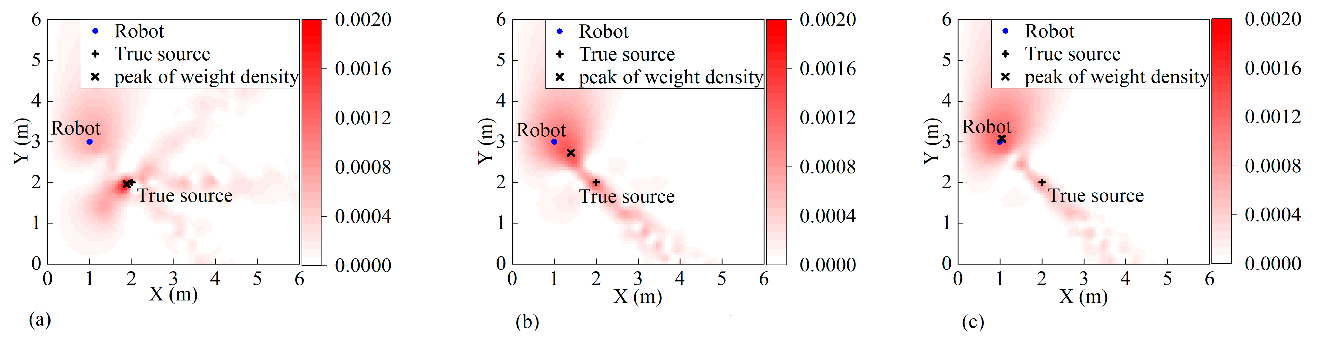
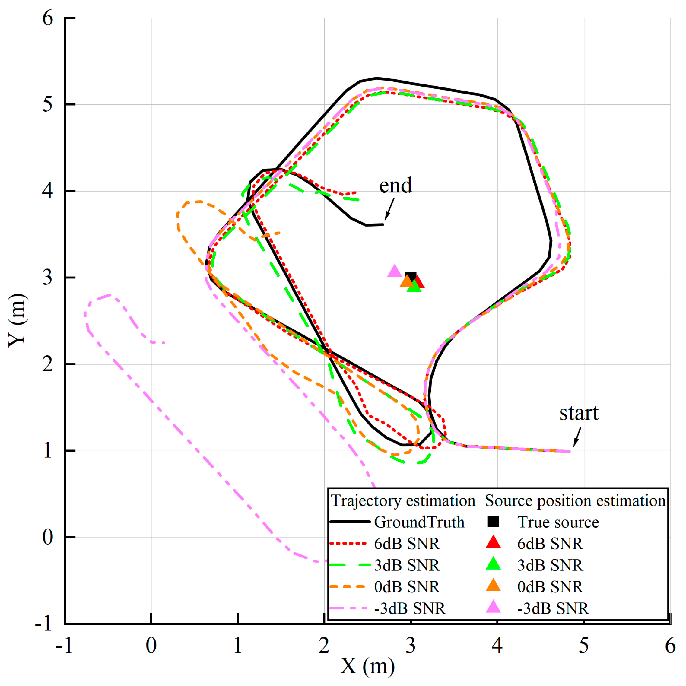
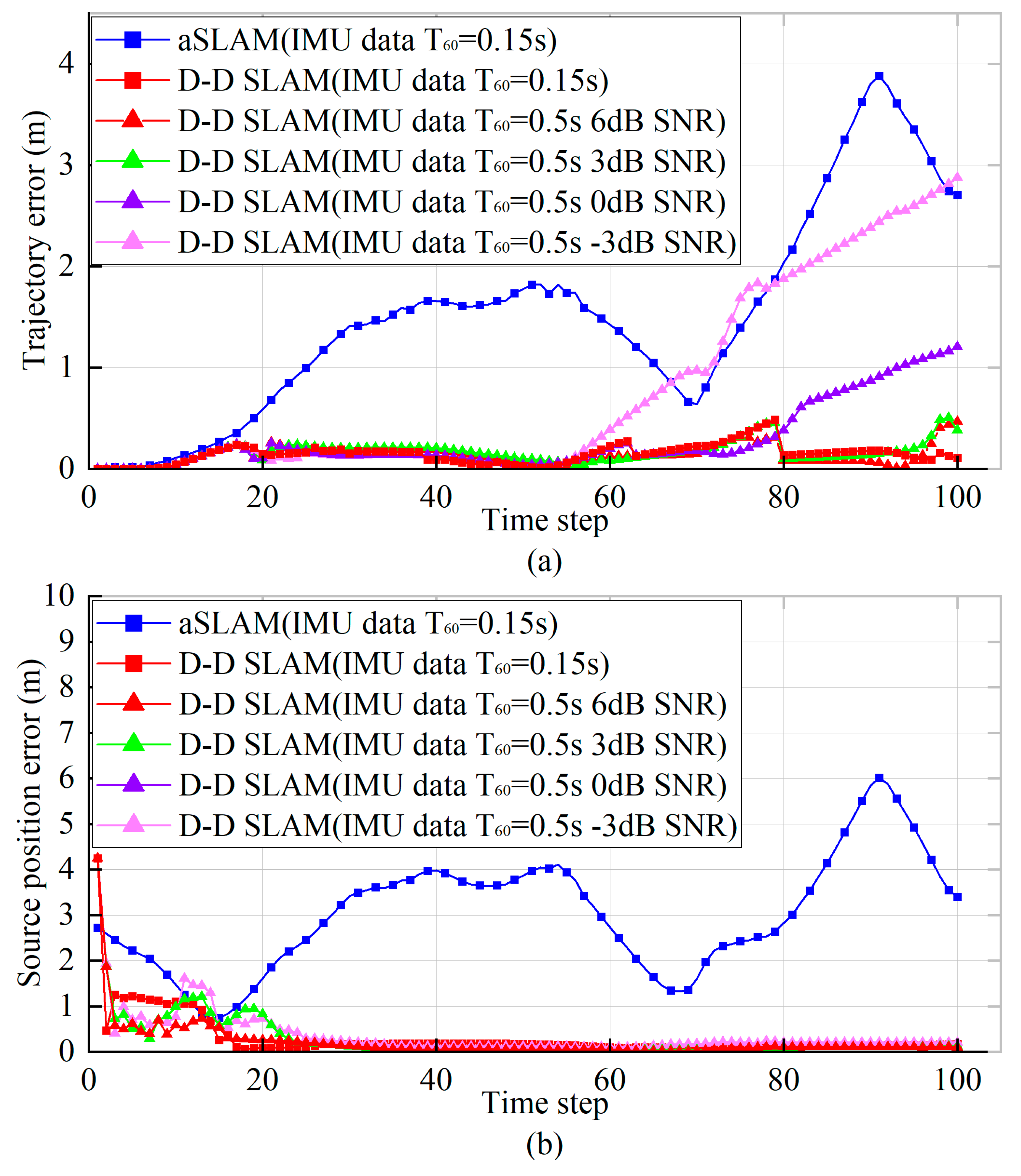
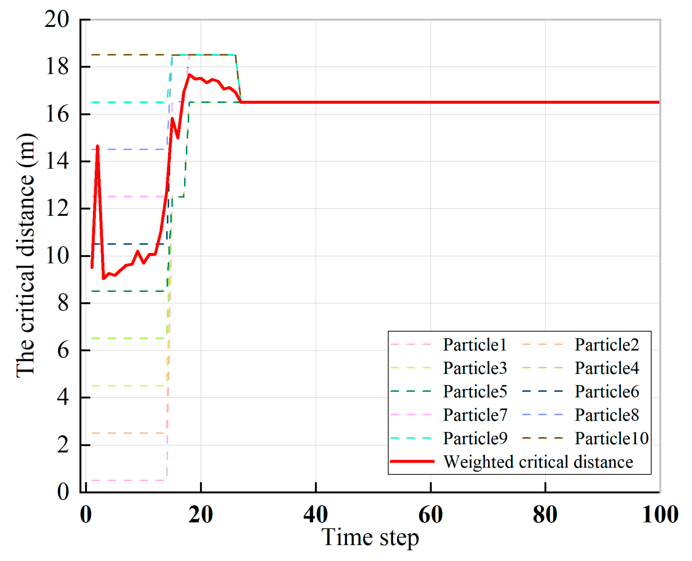
6.1. Simulation Results

The results of the aSLAM and the proposed D-D SLAM in the simulation are shown in Figure 3. The results of the D-D SLAM under different conditions are shown in Figure 4 and Figure 5, respectively. As shown in Figure 3 with the orange dashed-dotted line and solid circles, the trajectory and source position estimations of aSLAM with the true speed, which only contains Gaussian noise similar to that in [7], reach the expected effect, meeting the mean accuracies of 0.136 m and 0.14 m for estimations of the trajectory and source position, respectively.

However, when the simulated IMU data that contain nonlinear numerical error and Gaussian measurement noise are applied, aSLAM has poor performance. As shown by the blue dashed line in Figure 3, the trajectory estimation deviation increases with time. Within 29 s (29 time steps), the estimated position of the robot starts to be outside the room. The corresponding source position estimations are nonconvergent and sometimes even out of the room, so they cannot be marked as static points in Figure 3. In contrast, the proposed D-D SLAM with the same simulated IMU data performs well. As shown in Figure 3, the trajectory estimation of D-D SLAM in the red dotted line basically matches the ground truth, and the source position estimation in the red solid triangles is always close to the true source’s position. During the whole process of 100 s (100 time steps), the estimation of the trajectory and source position with the proposed D-D SLAM is convergent and stable.

The poor performance of aSLAM with IMU data implies that additional constraints are needed in this situation. As the nonlinear noise is due to the integration error of the IMU, the DRR is used to compute the source’s distance from the robot, which is applied as a new constraint. The result shown in Figure 3 demonstrates the different performances under the same conditions between aSLAM and the proposed D-D SLAM, proving the effectiveness of D-D SLAM. The use of the DRR for source distance estimations, which is considered an additional constraint, is key to eliminating the nonlinear error of IMU measurements.

Quantitative analysis of the accuracy using the Euler distance is illustrated in Figure 6. Under the condition of T₆₀ = 0.15 s, the result of aSLAM is drawn as a blue line with solid squares, while that of the proposed D-D SLAM is drawn as a red line with solid squares.

For aSLAM with IMU data, the trajectory error reaches a maximum of 3.9 m at 91 s (91 time steps), and its mean value is 1.55 m, as shown in Figure 6a. Moreover, the overall trend of its trajectory error increases over time. With the random initial source position, the corresponding source position estimation error is unstable, as shown in Figure 6b. The error also reaches a maximum of 6.0 m at 91 s (91 time steps), and its average is 3.0 m. Within a room of 6 m × 6 m × 3 m, the trajectory and source position errors are unacceptable.

For the proposed D-D SLAM with IMU data, the maximum trajectory error is less than 0.48 m, and the mean value of the trajectory error is 0.14 m. Meanwhile, the source position error is less than 0.19 m just after 16 s (16 time steps), even though the source position error at the beginning is quite large due to the random initial source position. Compared with aSLAM, the source position error of D-D SLAM converges faster even with the larger initial value of the source position error. These results show that the proposed D-D SLAM has better performance using the same simulated IMU measurement, which proves that D-D SLAM has stronger robustness for the nonlinear noise of motion reports.

The good performance of the proposed D-D SLAM relies on reliable source distance estimates, which are based on the accurate estimate of the critical distance d_c. However, d_c is initially unknown. With the online estimation method in this paper, d_c is calculated during the SLAM process. Different particles of critical distance d_c are initialized in the beginning, and the weight of each d_c particle is evaluated with the coincidence degree between the robot position, which corresponds to each d_c particle and the IMU measurements. During the SLAM procedure, those d_c particles whose corresponding robot position matches poorly with IMU measurements, DoA estimates, and sound source distance estimations from DRR are dropped. Figure 7 is the result of d_c at different time steps, where the different color dashed lines represent values of different d_c particles and the red solid line represents their weighted mean. The mean of d_c converges rapidly to a stable value in less than 27 s (27 time steps). The results show that the proposed online estimation method can obtain a convincing critical distance, even though the directivity of the source and receiver, the room size, and the reverberation time are unknown.

The reverberation time T₆₀ of the room is a general acoustic character of the environment. The simulation results of different reverberation times (T₆₀ = 0.15 s and T₆₀ = 0.5 s) are shown in Figure 3 and Figure 5, respectively. As shown in Figure 6, the average errors of trajectory and source position are 0.14 m and 0.21 m, respectively, when T₆₀ = 0. 5 s and SNR = 6 dB, while the average errors of trajectory and source position are 0.14 m and 0.29 m, respectively, when T₆₀ = 0. 15 s. In different acoustic environments, the proposed D-D SLAM still gets small errors and has similar performances, showing its robustness against changing the environment.

As shown in Figure 3 and Figure 5, the D-D SLAM can work with the continuous sound source of music or white noise, so the white noise sound source is unnecessary. The frequency ranges of the music and the white noise used in the simulation are different, and the frequency of the music is time-varying, so the D-D SLAM is insensitive to the frequency range.

The influences of different SNRs are studied. As shown in Figure 6, the average errors of trajectory and source position are 0.14 m and 0.21 m, respectively, when SNR = 6 dB, while the average errors of trajectory and source position are 0.16 m and 0.27 m, respectively, when SNR = 3 dB. The errors of trajectory estimation do not converge when SNRs are 0 dB and −3 dB. The trajectory error of −3 dB SNR grows faster than that of 0 dB SNR. Therefore, simulation results show that received signals whose SNR is bigger than 3 dB is necessary for the proposed technique.

In the simulation, the results of the D-D SLAM with and without the keyframe method are shown in Figure 4. The trajectory estimations of the D-D SLAM with and without the keyframe method are comparable before the robot remains stationary. The robot begins to remain stationary after moving for 20 time steps. After remaining stationary for 10 time steps, the trajectory estimations of the D-D SLAM without the keyframe method (blue line) go seriously wrong. And the source position estimations of the D-D SLAM without the keyframe method (blue triangle) are much closer to the position where the robot remains stationary rather than the position of the true source. This result is similar to the phenomenon presented in Figure 2. On the contrary, the D-D SLAM with the keyframe method (red line) still performs well after remaining stationary for 10 time steps. It is possible for a robot to remain stationary for some time during the SLAM procedure, so the keyframe method is necessary to prevent false source and trajectory estimations when the robot keeps still.

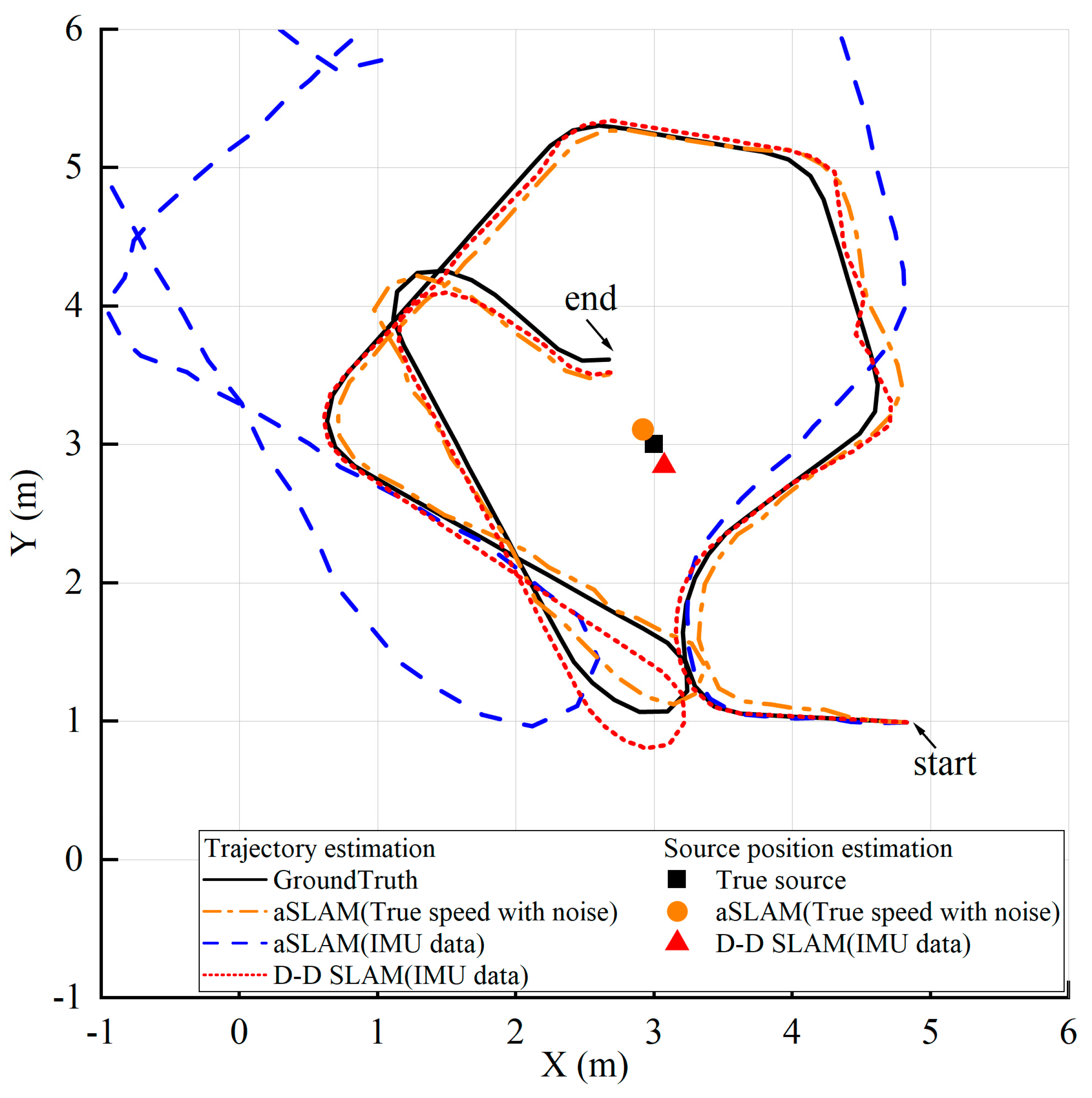
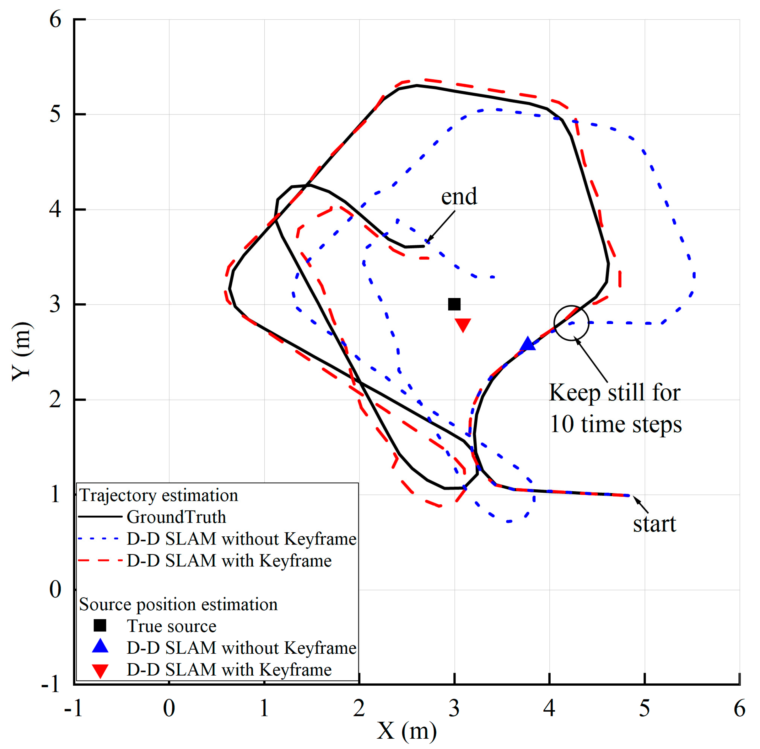
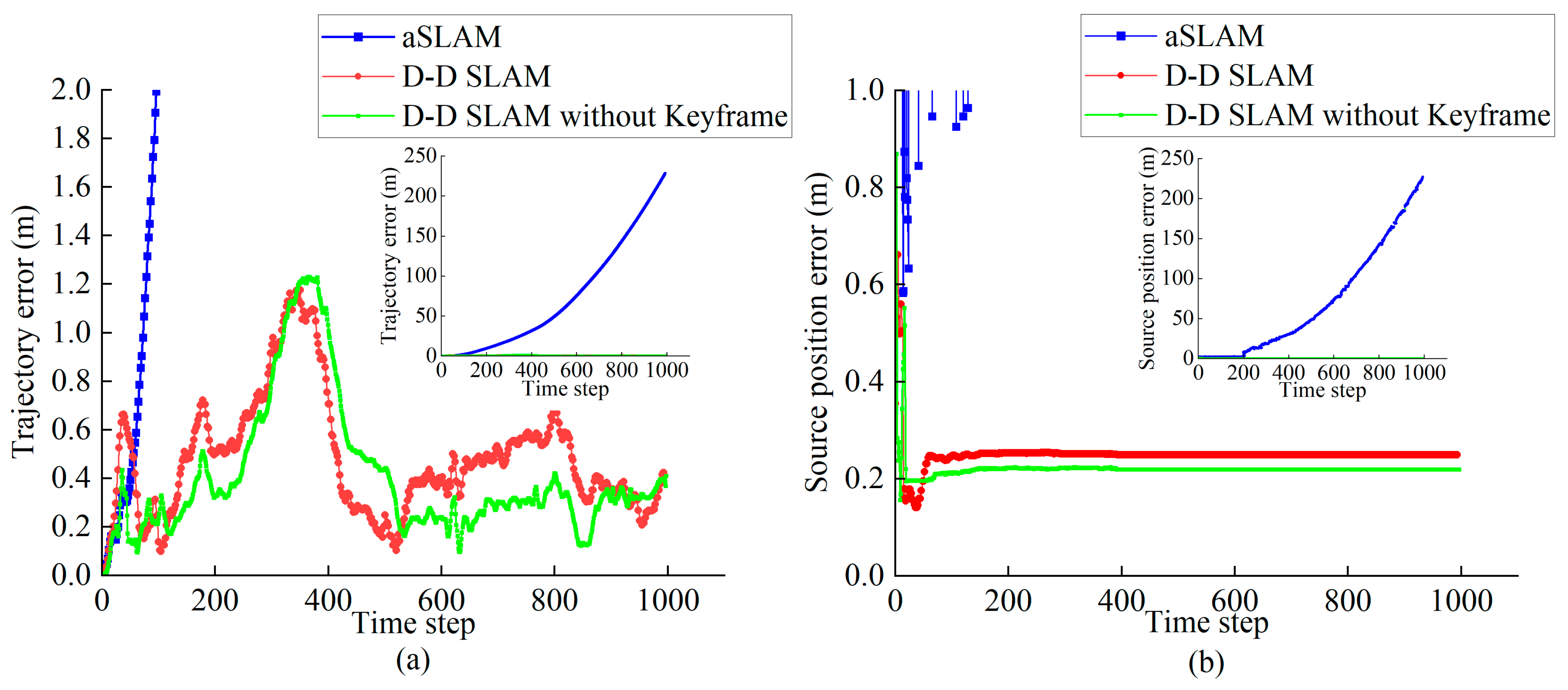
6.2. Experimental Results

Figure 8 shows the estimated trajectory and source position using D-D SLAM and aSLAM for real indoor datasets [15]. Even worse than that in simulation Group II, the estimated trajectory of aSLAM in the experiment goes outside the boundary of the experiment room after 18.7 s (402 time steps) and never returns during the remainder of the experiment. Therefore, it is not fully shown in Figure 8. The gradual divergence of the estimated trajectory is because of the shifting integrated velocity from the IMU measurements. Due to the incremental error of trajectory estimation, the source estimation of aSLAM is also unstable, and out of the room, so it cannot be marked in Figure 8. In contrast, the estimated trajectory of the proposed D-D SLAM always converges to a small neighborhood of the ground truth, as shown in Figure 8. Meanwhile, the estimation of the source position also converges with the true source position.

Figure 9 illustrates the estimation errors of the trajectory and source position. For aSLAM with real indoor data, the overall trajectory error tends to increase during the complete SLAM process, which is unacceptable. The source position error has the same trend as that of the trajectory error.

For the proposed D-D SLAM with the keyframe method, the maximum trajectory error reaches 1.18 m at 16.1 s (347 time steps), and its mean value is 0.48 m. In the meantime, the maximum error of the source position estimates of 0.66 m occurs at the beginning because the initial source position is random, and the error quickly converges to the stable value of 0.25 m after 2.8 s (60 time steps).

Compared with aSLAM, the proposed D-D SLAM has an acceptable performance in the trajectory and source position error, proving its validity for real world indoor scenes. The results in Figure 9 show the potential of the proposed D-D SLAM to work with an IMU in closed environments.

In the experiment, the results of the D-D SLAM with and without the keyframe method are shown in Figure 8, and the corresponding errors are shown in Figure 9. There are only small differences between the results of the D-D SLAM with and without the keyframe method. Thus, the keyframe method has a limited impact on the accuracy of estimations. Meanwhile, the use of the proposed D-D SLAM contributes to reducing the computing effort.

Figure 10 shows the critical distance estimation on the DREGON dataset. Similar to that in the simulation, the estimated critical distance converges rapidly to a stable value near 6.8 m.

With Intel i5-7500 CPU (4 cores 3.40GHz), under the condition of 10 particles, the expected latency is 0.1392 s, and the D-D SLAM performs at a speed of 7.1 FPS. The received audio signals do not change significantly when the microphone on the robot moves slightly, so the FPS of 7.1 should be acceptable for acoustic SLAM.

6.3. Analysis

In this section, the reasons for the trajectory errors are analyzed. The trajectory errors are affected by the number of particles, the max number of GM components used in source mapping, the DoA estimates, the IMU measurements, and the robot’s distance from the source.

The positional errors in different particle numbers are observed (as triangle and circle marks in Figure 11a). It is also important to determine the influence of the particle number on the critical distance estimation. The experiment in Section 5.2 is repeated for 5, 8, 10, 15, and 20 particles to investigate if a further improvement of the positional accuracy and the critical distance estimation can be achieved.

When the number of particles increases from 5 to 10, the errors of source position and robot trajectory estimation decline quickly because the brute force strategy consists of increasing the number of particles and proves to be effective [32]. When the number of particles increases above 10, the errors of the source position and the robot trajectory estimation stabilize at values of 0.25 m and 0.48 m, respectively. The reason for this is that the contribution of increasing the particle number is negligible after a few iterations [33]. The critical distance estimation also quickly converges to a stable value for the same reason.

The experiment in Section 5.2 is also repeated for different max numbers of GM components used in source mapping (as triangle and circle marks in Figure 11b). With an increase in the maximum of GM components, the positional error and the critical distance estimates quickly converge to a stable value.

As mentioned before, the SRP-PHAT with limited elevation search boundaries has high-accuracy DoA results. Even if the direction of the drone noise is in the range of the source direction, the Wiener Filter with the noise sample can be applied for noise reduction [15]. Incidentally, the drone noise can only affect the ITD and the coherence of binaural signals in the calculation process of DRR. As the ITD is calculated with accurate DoA estimates, the ITD is robust to drone noise. As the drone noise is diffuse and incoherent between different channels, it can be suppressed when calculating the coherence of binaural signals.

As the covariance of the DoA estimates and the IMU measurements are considered to be time-invariant while the trajectory errors have obvious variation with time, the time-varying robot’s distance from the source is considered. In Figure 12, the true robot-source distance is represented with the blue dashed line, and the trajectory error of D-D SLAM is drawn with the solid red line. What Figure 12 clearly shows is that the trajectory error increases with the decrease in the true robot-source distance. Roughly speaking, the trajectory error reaches the maximum when the true robot-source distance approaches the minimum. Therefore, it can be assumed that the trajectory error is associated with the robot-source distance.

Using (16), the estimation of the robot-source distance depends on the critical distance. The critical distance should be fixed when the reverberation field is stable. However, the reverberation field may vary if there are moving objects. The closer the robot is to the source, the larger its influence on the reverberation field. The reason is that when they are close, the multiple diffractions and the multiple reflections they cause will become stronger, and the influence on the reverberation field is also heavier, and vice versa.

As shown in Figure 10, when the robot is still far from the source, the critical distance estimation has already converged to a stable value, leading to particle dilution of the critical distance. After that, the variation in the reverberation field caused by the change in distance between the robot and the source can no longer be considered with the diluted particle filter. As a result, the outdated estimation of the critical distance will affect the estimation of the robot-source distance, according to (16). The deviation of the robot-source distance finally causes an increase in the trajectory estimation error.

7. Conclusions

Focusing on the solution of indoor SLAM with acoustic data and an IMU, D-D SLAM is proposed. With the keyframe method, D-D SLAM performs well in mapping regardless of whether the robot moves or remains stationary. The use of the DRR for the estimation of the source’s distance from the robot as a new constraint in D-D SLAM effectively eliminates the nonlinear noise of the IMU measurements. As the key factor to calculate the source’s distance from the DRR estimates, the critical distance is unknown initially, so a particle filter is applied to estimate the critical distance online, and the estimation of the critical distance converges to a stable value.

According to the results, D-D SLAM has good performance in both simulations and experiments. For the first time, an acoustic SLAM algorithm is validated with a real indoor dataset containing only acoustic data and IMU measurements. Different from previous work, D-D SLAM is designed for three-dimensional motion and rotation. On the real indoor dataset, the proposed D-D SLAM can locate the robot with an average accuracy of 0.48 m and build a source map with an average accuracy of 0.25 m. Even though the initial source position is random, the error of the source position converges to less than 0.25 m within 2.8 s.

These results demonstrate the effectiveness of the proposed D-D SLAM in real-world indoor scenes. In the future, D-D SLAM may contribute to robot localization and map building when conventional optical sensors are not suitable for special indoor environments, for example, foggy rooms where light and lasers cannot penetrate during navigation missions.

References

1. Qin, T.; Li, P.; Shen, S. VINS-Mono: A Robust and Versatile Monocular Visual-Inertial State Estimator. IEEE Trans. Robot. 2018, 34, 1004–1020. [Google Scholar] [CrossRef]
2. Chen, L.; Yang, A.; Hu, H.; Naeem, W. RBPF-MSIS: Toward Rao-Blackwellized Particle Filter SLAM for Autonomous Underwater Vehicle With Slow Mechanical Scanning Imaging Sonar. IEEE Syst. J. 2020, 14, 3301–3312. [Google Scholar] [CrossRef]
3. Shim, Y.; Park, J.; Kim, J. Relative navigation with passive underwater acoustic sensing. In Proceedings of the 2015 12th International Conference on Ubiquitous Robots and Ambient Intelligence (URAI), Goyang, Republic of Korea, 28–30 October 2015; pp. 214–217. [Google Scholar]
4. Ribas, D.; Ridao, P.; Tardós, J.D.; Neira, J. Underwater SLAM in Man-Made Structured Environments. J. Field Robot. 2008, 25, 898–921. Available online: https://onlinelibrary.wiley.com/doi/abs/10.1002/rob.20249 (accessed on 3 July 2021). [CrossRef]
5. Hu, J.S.; Chan, C.Y.; Wang, C.K.; Lee, M.T.; Kuo, C.Y. Simultaneous Localization of a Mobile Robot and Multiple Sound Sources Using a Microphone Array. Adv. Robot. 2011, 25, 135–152. [Google Scholar] [CrossRef]
6. Kallakuri, N.; Even, J.; Morales, Y.; Ishi, C.; Hagita, N. Probabilistic Approach for Building Auditory Maps with a Mobile Microphone Array. In Proceedings of the 2013 IEEE International Conference on Robotics and Automation (ICRA), Karlsruhe, Germany, 6–10 May 2013; pp. 2270–2275. [Google Scholar]
7. Evers, C.; Naylor, P.A. Acoustic SLAM. IEEE/ACM Trans. Audio Speech Lang. Process. 2018, 26, 1484–1498. [Google Scholar] [CrossRef]
8. Evers, C.; Naylor, P.A. Optimized Self-Localization for SLAM in Dynamic Scenes Using Probability Hypothesis Density Filters. IEEE Trans. Signal Process. 2018, 66, 863–878. [Google Scholar] [CrossRef]
9. Joly, C.; Rives, P. Bearing-only sam using a minimal inverse depth parametrization—Application to Omnidirectional SLAM. In Proceedings of the 7th International Conference on Informatics in Control, Automation and Robotics, Funchal, Portugal, 15–18 June 2010; pp. 281–288. [Google Scholar] [CrossRef]
10. Rascon, C.; Meza, I. Localization of sound sources in robotics: A review. Robot. Auton. Syst. 2017, 96, 184–210. [Google Scholar] [CrossRef]
11. Sobhdel, A.; Shahrivari, S. Few-Shot Sound Source Distance Estimation Using Relation Networks. arXiv 2019, arXiv:2109.10561. [Google Scholar] [CrossRef]
12. Yiwere, M.; Rhee, E.J. Sound Source Distance Estimation Using Deep Learning: An Image Classification Approach. Sensors 2019, 20, 172. [Google Scholar] [CrossRef] [Green Version]
13. Portello, P.; Danès, P.; Argentieri, S. Acoustic models and Kalman filtering strategies for active binaural sound localization. In Proceedings of the 2011 IEEE/RSJ International Conference on Intelligent Robots and Systems, San Francisco, CA, USA, 25–30 September 2011; pp. 137–142. [Google Scholar] [CrossRef]
14. Zahorik, P. Direct-to-reverberant energy ratio sensitivity. J. Acoust. Soc. Am. 2002, 112, 2110–2117. [Google Scholar] [CrossRef]
15. Strauss, M.; Mordel, P.; Miguet, V.; Deleforge, A. DREGON: Dataset and Methods for UAV-Embedded Sound Source Localization. In Proceedings of the 2018 IEEE/RSJ International Conference on Intelligent Robots and Systems (IROS), Madrid, Spain, 1–5 October 2018; pp. 1–8. [Google Scholar] [CrossRef]
16. Zohourian, M.; Martin, R. Binaural Direct-to-Reverberant Energy Ratio and Speaker Distance Estimation. IEEE/ACM Trans. Audio Speech Lang. Process. 2020, 28, 92–104. [Google Scholar] [CrossRef]
17. Forster, C.; Carlone, L.; Dellaert, F.; Scaramuzza, D. IMU Preintegration on Manifold for Efficient Visual-Inertial Maximum-a-Posteriori Estimation. Robotics Sci. Syst. 2015. [Google Scholar] [CrossRef]
18. Le Gentil, C.; Vidal-Calleja, T.A.; Huang, S. Gaussian Process Preintegration for Inertial-Aided State Estimation. IEEE Robot. Autom. Lett. 2020, 5, 2108–2114. [Google Scholar] [CrossRef]
19. Communication Acoustics; Springer: Berlin/Heidelberg, Germany. Available online: https://link.springer.com/book/10.1007/b139075 (accessed on 7 July 2021).
20. Schwartz, O.; Plinge, A.; Habets, E.A.P.; Gannot, S. Blind microphone geometry calibration using one reverberant speech event. In Proceedings of the 2017 IEEE Workshop on Applications of Signal Processing to Audio and Acoustics (WASPAA), New Paltz, NY, USA, 15–18 October 2017; pp. 131–135. [Google Scholar] [CrossRef]
21. Khairuddin, R.; Talib, M.; Haron, H. Review on simultaneous localization and mapping (SLAM). In Proceedings of the 2015 IEEE International Conference on Control System, Computing and Engineering (ICCSCE), Penang, Malaysia, 27–29 November 2015; pp. 85–90. [Google Scholar] [CrossRef]
22. Vo, B.-N.; Ma, W.-K. The Gaussian Mixture Probability Hypothesis Density Filter. IEEE Trans. Signal Process. 2006, 54, 4091–4104. [Google Scholar] [CrossRef]
23. Ristic, B.; Vo, B.-N.; Clark, D. A Metric for Performance Evaluation of Multi-Target Tracking Algorithms. IEEE Trans. Signal Process. 2011, 59, 3452–3457. [Google Scholar] [CrossRef]
24. Casella, G.; Robert, C.P. Rao-Blackwellisation of Sampling Schemes. Biometrika 1996, 83, 81–94. [Google Scholar] [CrossRef]
25. Schon, T.; Gustafsson, F.; Nordlund, P.-J. Marginalized particle filters for mixed linear/nonlinear state-space models. IEEE Trans. Signal Process. 2005, 53, 2279–2289. [Google Scholar] [CrossRef]
26. Jwo, D.-J.; Cho, T.-S. Critical remarks on the linearised and extended Kalman filters with geodetic navigation examples. Measurement 2010, 43, 1077–1089. [Google Scholar] [CrossRef]
27. Salmond, D.J. Mixture Reduction Algorithms for Point and Extended Object Tracking in Clutter. IEEE Trans. Aerosp. Electron. Syst. 2009, 45, 667–686. [Google Scholar] [CrossRef]
28. Arulampalam, M.; Maskell, S.; Gordon, N.; Clapp, T. A tutorial on particle filters for online nonlinear/non-Gaussian Bayesian tracking. IEEE Trans. Signal Process. 2002, 50, 174–188. [Google Scholar] [CrossRef]
29. Lehmann, E.A.; Johansson, A.M. Diffuse Reverberation Model for Efficient Image-Source Simulation of Room Impulse Responses. IEEE Trans. Audio Speech Lang. Process. 2010, 18, 1429–1439. [Google Scholar] [CrossRef]
30. Vincent, C.E.; Roomsimove, A. Matlab Toolbox for the Computation of Simulated Room Impulses Responses for Moving Sources. Available online: http://www.irisa.fr/metiss/members/evincent/software (accessed on 27 October 2020).
31. DiBiase, J.H.; Silverman, H.; Brandstein, M.S. Robust localization in reverberant rooms. In Microphone Arrays: Signal Processing Techniques and Applications; Springer: Berlin/Heidelberg, Germany, 2001. [Google Scholar]
32. Liang, Y.; Feng, Y.; Quan, P.; Yan, L. Adaptive Particle Filter: Tuning Particle Number and Sampling Interval. In Proceedings of the 24th Chinese Control Conference, Guangzhou, China, 15 June–18 July 2005; Volumes 1 and 2, pp. 803–807. [Google Scholar]
33. Kuptametee, C.; Aunsri, N. A review of resampling techniques in particle filtering framework. Measurement 2022, 193, 110836. [Google Scholar] [CrossRef]
Figure 1. World frame and robot frame.
Drones 07 00120 g001
Figure 2. Extensive simulation of the origin method when the robot and the source remain still for (a) beginning (3 time steps), (b) 10 time steps, and (c) 17 time steps.
Drones 07 00120 g002
Figure 3. T60 = 0.15 s, Trajectory estimation on simulations for aSLAM with true speed plus noise (orange dash-dotted line), aSLAM with IMU data (blue dashed line), and the D-D SLAM with IMU data (red dotted line).
Drones 07 00120 g003
Figure 4. T60 = 0.15 s, Trajectory and source estimations on simulations for D-D SLAM with and without the keyframe method.
Drones 07 00120 g004
Figure 5. T60 = 0.5 s, Trajectory and source estimations on simulations for D-D SLAM under the condition of different SNRs.
Drones 07 00120 g005
Figure 6. Simulation results for (a) the trajectory errors and (b) the source position errors over time steps.
Drones 07 00120 g006
Figure 7. The state of different critical distance particles and the weighted critical distance with simulation data under the condition of T60 = 0.15 s.
Drones 07 00120 g007
Figure 8. The estimation of trajectory and the source position using aSLAM and D-D SLAM with and without the keyframe method.
Drones 07 00120 g008
Figure 9. Dataset result for (a) the trajectory error and (b) the source position estimation error over time steps.
Drones 07 00120 g009
Figure 10. The state of different critical distance particles and the weighted critical distance with real data.
Drones 07 00120 g010
Figure 11. The positional error and the critical distance estimation with (a) different numbers of particles and (b) the max number of GM components.
Drones 07 00120 g011
Figure 12. The robot-source distance and the trajectory error of D-D SLAM.
Drones 07 00120 g012
Disclaimer/Publisher’s Note: The statements, opinions and data contained in all publications are solely those of the individual author(s) and contributor(s) and not of MDPI and/or the editor(s). MDPI and/or the editor(s) disclaim responsibility for any injury to people or property resulting from any ideas, methods, instructions or products referred to in the content.