Abstract
The purpose of this paper is the evaluation of the aero-propulsive effects on a UAV wing model with distributed propulsion. An array of three propellers is placed ahead of the leading edge of a rectangular wing with flap. The investigation was performed with high-fidelity numerical analyses to provide insights into the phenomenology and to screen the interesting positions to be validated in the wind tunnel. The propellers’ array is moved into twelve different positions, allowing longitudinal and vertical translations. The wing has an untwisted and constant section profile, with a single slot trailing-edge flap that is deflected into three positions. The flap span is entirely covered by the propellers’ blowing. Results show an increment of lift, drag, and pitching moment coefficients with distributed propellers enabled. For a given thrust level, the magnitude of such increments depends on the propellers’ positions, the flap configuration, and the angle of attack. The lift enhancement sought in distributed propulsion applications comes at the expense of a significant increase in drag and pitching moment magnitude. In some combinations, the wing’s contribution to the aircraft longitudinal stability is severely affected. Conversely, the propellers’ inflow is altered such that thrust is increased in all the investigated configurations, with a small reduction of propulsive efficiency.
PACS:
47.85.Gj
1. Introduction
Among the several challenges in airplane and UAV design, improvements in aerodynamics can undoubtedly provide significant impact on the whole aircraft performance [1,2,3]. During the last decade, distributed propulsion has been one of the most investigated technologies. It can be defined as a propulsion system where the vehicle thrust is produced from an array of propulsors located across the air vehicle [4]. An interesting type of distributed propulsion, which is currently being studied across various research and industry organizations, is a system where electrical energy sources are connected via transmission lines to multiple electric motor-driven propulsors. This system is called Distributed Electric Propulsion (DEP) and has the potential to introduce substantial improvements in future air-vehicle performance, efficiency, and robustness.
Distributed propulsion is not an entirely new idea. Ref. [5] describes the use of a jet-wing distributed propulsion to cancel the drag by filling the wake to increase the propulsive efficiency. This falls under the broader topic of boundary layer ingestion [6], with recent investigations supporting its application with distributed propulsion [7,8,9].
DEP can be employed to provide both the required thrust for flight and additional advantages associated with synergistic propulsion–airframe integration. Its use is widely spread in urban air mobility research [10,11,12] as well as in current electric VTOL prototypes [13]. It is also an attractive technology as a directional control device in addition to the rudder [14,15,16,17].
DEP provides an increase of cruise efficiency of small aircraft through different types of interactions such as: increasing the dynamic pressure over the wing above free-stream during approach to allow for increased design wing loading (high-lift propeller), as well as reducing induced drag by installing propellers at the wing tips (wingtip propeller) [18].
The first interaction exploits the propwash upstream of the wing. In this way, the wing sections in the propellers’ slipstream experience an increase in flow speed such that their lift increases, making the wing more effective at low speeds. The LEAPTech (Leading Edge Asynchronous Propeller Technology) experiment was one of the earliest investigation on this effect [19]. The aerodynamic system analyzed was a wing designed for a four-seats general aviation aircraft with high wing loading to reduce cruise drag and improve handling quality. Several steady-state RANS simulations were performed with the propellers modeled as virtual disks and successfully validated with experimental tests [20].
Moreover, another computational study related to this experimental apparatus showed that there was a large benefit in lift coefficient over the entire investigated range of angle of attack, by using co-rotating distributed propellers spinning in the opposite direction of the wingtip vortex (inboard-up), instead of counter-rotating propellers. This benefit was quantified from a maximum lift coefficient amplified by a factor of 2.4 with respect to the unblown condition [21].
Della Vecchia et al. [22] evaluated the wing high-lift propellers’ effect on the Tecnam P2006T baseline wing, evenly splitting the available power of 200 hp through several distributed propellers and considering 120 hp needed for cruise tip-mounted propellers. Results showed a mild lift increment of about 1.0–1.5. This limited value was attributed to low engine power, reduced blowing, excessive wing planform area, and conventional propellers used for high lift. Moreover, the propeller diameter-to-chord ratio, which is a key parameter, was about the half of the value of the NASA X-57 Maxwell [23].
The effects of DEP on aircraft sizing and emissions was discussed by the authors in Refs. [24,25]. In these papers, it was remarked that DEP as a mean to enhance the airplane’s high-lift capabilities is not effective on all aircraft categories. Benefits are enabled on small aircraft within a range below 300 nmi, mainly because of the low energy density of batteries.
Surrogate models to predict the aero-acoustic performance of propellers have been presented by Poggi et al. [26], who claimed to predict performance and noise with a high level of accuracy on single as well as on distributed propellers. However, their application was focused on the urban air mobility scale and isolated propellers.
The effects of aerodynamic interactions between adjacent propellers have been experimentally investigated by De Vries et al. [27]. Their model was a constant section wing spanning the wind tunnel walls, with three propellers located around the mid plane. Their work did not consider change in propellers’ position, but was focused on the interactions among propellers to estimate changes in performance and noise with respect to the standalone case. They highlighted a small reduction of the efficiency of the middle propeller, showing that this effect was independent of the rotation direction and increased with angle of attack and staggering of the propeller-nacelle group.
Keller [28] investigated the use of DEP on the wing of a typical regional turboprop aircraft and showed results that surprisingly were not negatively impacting the cruise operations. In fact, a detrimental effect of cruise performance was expected because of the additional drag on the wing surface due to the blowing propellers. It is probable that this detrimental effect was mitigated by the limited thrust available and by the wingtip propellers. However, Keller attributed this to the absolute distance between the 12 distributed propeller disks and the wing, shorter than that of the standard twin-engines configuration. Conversely, take-off condition provided an increase of lift coefficient between 70% and 90%, without and with leading edge modification, respectively.
The integration of distributed propellers and the optimization of the aerodynamic design with a wing was described by Wang et al. [29], who highlighted how propeller spacing and disc loading affected the aerodynamic performance of the system.
The effects of DEP on wing aerodynamics were also investigated by Chen and Zhou [30], who developed an algorithm for the inverse design of distributed propeller according to desired slipstream shape. They have shown improvements of wing aerodynamic performance with respect to the minimum induced loss propeller design. They provided observations similar to the work of Patterson [18] and showed that the effect of three distributed propellers is not the sum of the effects of the three single propellers.
The first indications of the effects of propellers’ location are given by Gentry et al. [31], who tested a scaled semi-span wing model with flaps and a single propeller engine in a subsonic wind tunnel. They have shown that decreasing the propeller inclination (nose-down) enhanced the lift coefficient more than any horizontal or vertical displacement of the propulsive system. They also reported an additional increase in lift and drag with increasing propeller rotation speed—hence, thrust—and flap deflection.
Another systematic investigation of the effects of propellers’ positions and orientations was performed by Fei et al. [32], who tested a rectangular wing model with a plain flap spanning the entire wind tunnel height, one electric motor, and two propellers of different diameters. They highlighted the predominance of the vertical displacement of the propulsive system over the horizontal offset, although they found a different trend with the propeller’s inclination with respect to Ref. [31], probably because of the different thrust level of their model. They also showed a linear relationship between the unblown lift coefficient and the vertical position of the propeller, giving the maximum effective lift coefficient for each angle of attack. The effective lift coefficient was calculated from the total measured forces and it included both the wing aerodynamic lift and the propellers’ forces components in the direction of lift.
However, these last two references are not fully representative of a wing with distributed propellers, because of the single motor installed over the entire wingspan. More recently, the work of Serrano et al. [33] showed the effect of a propellers’ array behind the wing of a 25 kg fixed-wing unmanned aircraft, with the objective to investigate a practical way to enable boundary layer ingestion and provide thrust for such a machine. The paper is about a numerical investigation of a wing section with an actuator disk immediately behind the trailing edge. The limitation of the analysis to a wing section makes the results representative of a wing of infinite aspect ratio with an infinite array of distributed propellers. Moreover, they only investigated the effect of the vertical position of the propeller and mainly provided indications on the airfoil pressure coefficient distribution. Their work was extended with a proper orthogonal decomposition analysis to provide a surrogate model to estimate the lift coefficient with other propeller positions [34], but this does not add indications on the effects of other geometric parameters.
De Rosa et al. [35] numerically investigated the effects of propeller diameter-over-wing chord ratio and propeller thrust coefficient on the wing lift and drag aerodynamic coefficients. Their model is a flapped wing section with a virtual disk ahead of the leading edge and periodic conditions on the lateral walls to simulate an infinite array of co-rotating distributed propellers. Their work confirmed the expected results of an increase in both lift and drag coefficients with diameter-to-chord ratio and thrust coefficient until stall occurrence. More interesting is the relationship between the derived quantity thrust-coefficient-over-squared-advance-ratio with different airspeed values, which provided continuity of the curves. As expected, the largest lift increments were obtained at low speed. They also provided a method to estimate lift and drag coefficients as a function of the above-cited parameters. However, they did not investigate the effects of propeller position and most of the data are related to one flap deflection representing the take-off condition.
So far, the literature review highlighted the following key factors to exploit the benefits of distributed propulsion:
- The operative speed must be as low as possible;
- The thrust levels must be as high as possible;
- The propeller diameter-over-wing chord ratio should be close to unity;
- The propeller design should have an axial induction factor as constant as possible over the blade span;
- The propeller interaction with wing and high-lift devices must be carefully investigated with high-fidelity methods.
Moreover, there are some points that have not been adequately treated in literature, namely:
- The effects of the position of distributed propellers’ array on a three-dimensional wing, not just a wing section with a single propeller;
- The effects of different flap deflections on such a configuration, including chordwise and spanwise aerodynamic loadings;
- The effects of the aero-propulsive interactions on the wing pitching moment coefficient, often overlooked, but of extreme importance for aircraft stability and control;
- The mutual effect of the wing on the propeller, which is affected by the flowfield around it.
This paper provides a deep insight into these phenomenona, outlining the main aspects and criticalities of the above-cited issues. For this reason, the model was made up of a wing with three leading-edge propellers and a single-slotted flap. The effect of the propellers’ position was investigated by moving them in the longitudinal plane, together with three flap settings (i.e., retracted, take-off, and landing).
The remainder of the text is divided as follows. Section 2 describes the numerical model and the test matrix for three different flap deflections. After a grid convergence study, a design exploration on the flap position in unblown conditions is presented. Once the mesh refinement and the flap characteristics (gap, overlap, hinge line) were established, the numerical analyses were performed. Section 3 provides a discussion on the numerical exploration of the aero-propulsive effects due to the propellers’ array position. For each flap deflection there is a dedicated subsection, which in turn is divided into three parts: global effects, local effects, and wing-to-propeller effects. The global effects concern the influence of the propellers’ wake on the wing aerodynamic coefficients. Local effects deal with wing spanwise loading and chordwise pressure distributions affected by propellers’ slipstream, due to both axial and tangential flow acceleration. Wing-to-propeller effects refer to the wing-induced flow field on the propellers’ disks, which is different from the case of the isolated propeller. Finally, conclusions are drawn in Section 4.
2. Numerical Setup
The test model is a simple rectangular wing with a slotted flap covering about 64% of the wing span. The wing section is a LS(1)-0417 airfoil [36,37] with a 30% flap-chord ratio and an aspect ratio equal to 7. The short aspect ratio, which is below the usual values for fixed-wing UAVs [1], is due to the need to investigate the same model in a low-speed wind tunnel at a sufficient Reynolds number in the near future. A drawing of the wing half-model is given in Figure 1. Geometric details are reported in Table 1.
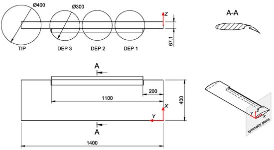
Figure 1.
Drawing of the starboard half-wing model with propellers’ disks. Units in mm.

Table 1.
Geometrical characteristics of the analyzed wing model.
There are three high-lift propellers with a diameter-to-chord ratio of 0.75 and positioned ahead of the wing, spanning the same wing area covered by the single slotted flap. These propellers have been analyzed in three horizontal (X) and four vertical (Z) positions, while their spanwise location (Y) is fixed (see Table 2). Figure 2 illustrates the matrix of the positions investigated in the longitudinal plane. The term “baseline location” indicates the initial position to which all other positions are referred. A wingtip propeller disk with unit diameter-to-chord ratio is also shown in Figure 1, but the analyses on such configuration are not discussed in this paper for the sake of brevity. Table 3 shows the test matrix.
Table 2.
Fixed spanwise positions of the propellers.
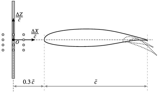
Figure 2.
Positions of the propellers’ array. The black circle is the baseline location.
Table 3.
Test matrix. All displacements are referred to the baseline location indicated in Figure 2.
The numerical wing model is not representative of a specific UAV, although it may be the baseline main lifting surface of a hypothetical 50 kg full-electric aircraft with distributed propulsion and wingtip propeller. As previously stated, the wing computational model has the same geometric characteristics of a physical model to be tested in the wind tunnel. Therefore, the numerical simulations are preliminary analyses for the real test article. In the conceptual design phase of this work, there were no detailed information on the internal structure and systems arrangement of the real model. For this reason, propellers were simulated with actuator disks, while nacelle were neglected. Their detailed design came at a later stage and it is topic for an experimental scientific article. Nonetheless, a preliminary sizing has been performed from the assigned diameter and the expected maximum motor shaft power. Details are given in Section 2.3.
The CFD package used for the simulations is Simcenter STAR-CCM+. Details on the mesh and on the physics are given in the following subsections. The application of CFD to high-lift prediction and propeller-wing interaction had been previously validated by the authors [22]. Ideally, the wind tunnel will operate at a flow speed of 20 m/s, corresponding to a Reynolds number based on the mean aerodynamic chord in standard conditions.
A preliminary two-dimensional numerical analysis was performed to explore the combined effect of flap gap, overlap, and deflection on the aerodynamic coefficients, without propeller effects. Once the virtual hinge for the flap’s deflection was fixed, three-dimensional simulations on the wing half-model were performed to investigate the effects of the position of the distributed propellers’ array at several flap deflections.
2.1. Two-Dimensional Flap Design Exploration
Although the focus of the work is on a three-dimensional design exploration, it appeared appropriate to perform a two-dimensional exploration on the flap position and deflection. These simulations are all in prop-off condition. In this way, the effects of propeller blowing on the three-dimensional model will be fairly compared to the best flap setup in unblown condition.
The mesh is made up of polygonal cells, with 20 prismatic layers extruded from the airfoil wall to capture the boundary layer. The prism layer total thickness and the first cell height is such to get a non-dimensional wall distance . The flow is modeled as steady and fully turbulent with the Spalart-Allmaras model [38,39]. The farfield is located at about 50 chords length from the airfoil. Despite the relatively low Reynolds number, it was decided to perform fully turbulent simulations for several reasons: the value of 530,000 can be matched in low-speed wind tunnel tests, but it is not representative of the full-scale (hypothetical) aircraft; wind tunnel tests require the application of roughness to force the flow transition; leading edge contamination as well as propellers’ slipstream may easily destroy the laminar flow on the real aircraft; and the results provided with a fully turbulent flow are easily extendable to larger aircraft.
A grid convergence study [40] was performed on the initial geometry to evaluate discretization errors. The fine mesh has a grid-convergence index (GCI) of less than 5% on both lift and pitching moment coefficients at stall, with an order of accuracy of about 0.6. Such grid is shown in Figure 3 and it has 323,000 cells. Then, the design exploration on flap gap, overlap, and deflection , whose definitions are illustrated in Figure 4, was performed. Figure 5 shows the contour of lift, drag, and pitching moment coefficients at angle of attack with the flap deflected by and , representing take-off and landing conditions, respectively, as a function of the flap’s non-dimensional displacements from an initial position. The initial and final values of the flap hinge line coordinates are reported in Table 4. The best design is a compromise between performance at take-off and landing. The final values of gap and overlap are reported in Table 5.
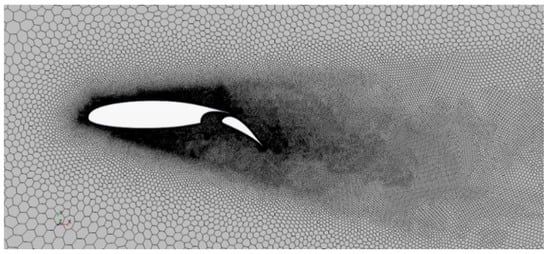
Figure 3.
Two-dimensional fine mesh around the airfoil. A conical-shaped refinement has been applied to capture the wake.
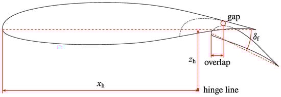
Figure 4.
Definitions of flap deflection , gap, overlap, and hinge line.
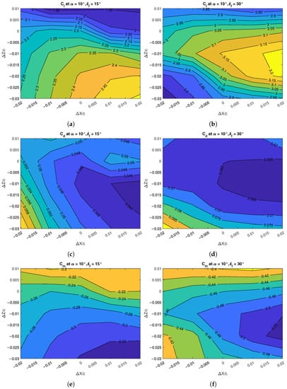
Figure 5.
Two-dimensional design exploration for flap position at : (a) lift coefficient in take-off; (b) lift coefficient in landing; (c) drag coefficient in take-off; (d) drag coefficient in landing; (e) pitching moment coefficient in take-off; (f) pitching moment coefficient in landing.
Table 4.
Baseline and final coordinates of flap hinge line. Symbols are defined in Figure 4.
Table 5.
Flap deflections with final values of gap and overlap. Their definition is illustrated in Figure 4.
2.2. Three-Dimensional Grid Convergence Study
Once the flap hinge position was fixed, a new grid convergence investigation was performed on the three-dimensional mesh in prop-off condition. Again, the study of the discretization error was performed using the GCI method [40]. The computational domain is illustrated in Figure 6. The simulations were symmetric about the longitudinal plane at the root airfoil. All the meshes were made up of polyhedral cells with a layer of 20 prismatic cells extruded from the wing surface to capture the boundary layer. The number of both core and prism layer cells changed within the grid convergence investigation, but the thickness of the prism layer had been held constant to m with the first layer m thick to keep the non-dimensional wall height on most of the wing surface. The fine mesh with more than 8 million cells is illustrated in Figure 7. The max discretization error was less than 3% for the lift and pitching moment coefficient, while it was below 6% for the drag coefficient. The effects on grid refinements on the aerodynamic coefficients at three angles of attack are reported in Figure 8.
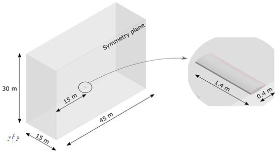
Figure 6.
Computational domain.
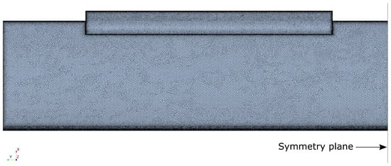
Figure 7.
Top view of the finest mesh on the wing model with flap.
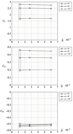
Figure 8.
Grid convergence investigation on the three-dimensional half-wing model with flap. N is the number of cells. The chosen mesh has . The related data points are enclosed by gray rectangles.
2.3. Simulation of the Propellers
Propellers were simulated with the virtual disk model of Simcenter STAR-CCM+, which is a two-way interaction actuator disk model with swirl. The radial distributions of thrust and torque were not constant, but followed the Goldstein distribution [41]. Two-way interaction means that the propeller affects the wing aerodynamics and vice versa. The three distributed propellers had a diameter of 0.30 m and a hub diameter of 0.035 m. The area within the hub’s circle did not belong to the virtual disk; hence, the flow was not accelerated there.
Propeller performance was measured by the following variables:
where is the free-stream flow speed, n is the propeller rotational rate in s, D is the propeller diameter, is the free-stream flow density, T is the propeller thrust, and P is the propeller shaft power. The above defined quantities are the advance ratio J, the thrust coefficient , the power coefficient , and the propeller efficiency .
A preliminary design of the propellers was made to provide an axial flow speed increment of about 20%, which should be easily achievable in the future wind tunnel tests. The propeller was designed with XROTOR [42] to operate in standard conditions at a constant flow speed m/s, providing a thrust N at 7000 RPM with five blades. The blade section was a modified Clark-Y airfoil scaled to 18% relative thickness and 1.5% chord length open trailing edge for ease of future manufacturing. Airfoil aerodynamic characteristics were evaluated with XFOIL [43] at Reynolds numbers between 50,000 and 100,000. These data were imported into XROTOR, using its vortex formulation to calculate induced velocities and induced losses. This approach was validated in Refs. [44,45,46], where vortex codes were expected to provide a 10% discrepancy in thrust and power coefficients with respect to CFD solvers using the moving reference frame method. The standalone propeller performance coefficients were evaluated with XROTOR and are shown in Figure 9. These were the input data for the virtual disk model of STAR-CCM+. The reference set point for the numerical analyses is given in Table 6 for comparison with the wing–propeller interactions that will be discussed in the next sections.
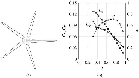
Figure 9.
High-lift propeller designed with XROTOR: (a) propeller planform; (b) propeller characteristics.
Table 6.
Operating point for the distributed propellers evaluated with XROTOR.
3. Effects of the Position of the Distributed Propellers
In this section, the effects of the position of the distributed propellers’ array are discussed. Three flap configurations had been investigated (retracted, take-off, and landing), presented in Section 3.1, Section 3.2 and Section 3.3. For each configuration, a comparison is made between prop-on and prop-off conditions, with a focus on the increments of aerodynamic coefficients at specific angles of attack. Details on spanwise and chordwise load distributions are also given. Nomenclature for the charts’ legend are reported in Table 3. The relative wing-DEP array position has been illustrated in Figure 2.
3.1. Flap Retracted (Cruise Conditions)
Data about the clean wing are here presented and discussed. This subsection is divided into three parts concerning: the effects of the propellers on the aerodynamic coefficients; the effects of the propellers on the aerodynamic loads; and the effects of the wing on the propellers’ performance.
3.1.1. Global Effects of the Propellers on the Wing Aerodynamics
The effects of distributed propulsion on the wing aerodynamics in clean configuration are shown in Figure 10. It is apparent an increase of the magnitude of the aerodynamic coefficients on all the investigated propellers’ positions. More specifically, in the linear range of the lift curve, there was an increment of both the lift coefficient and its slope (Figure 10a). This is attributed to the additional local flow velocity due to the propellers’ blowing, providing more lift force for a given angle of attack and planform area, whereas the lift coefficient was still referred to the free-stream value of the dynamic pressure. That is because the wing profiles were more cambered and their chords were stretched. In fact, camber provides the shift of the lift curve, whereas the (virtual) additional area provides the increment in lift curve slope.
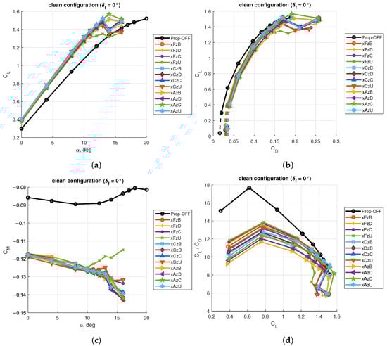
Figure 10.
Aerodynamic coefficients for the clean wing: (a) lift curves; (b) drag polars; (c) pitching moment curves; (d) aerodynamic efficiency curves.
With propellers enabled, the drag polar curves were shifted to higher values of the drag coefficient (Figure 10b). The curves were also extrapolated to lower values of the lift coefficient with the modified parabolic drag polar expression:
where the values of and were estimated with a second order best fit curve on the data within the range . The extended curves are represented with dashed lines with the same colors and markers of the available data.
Thus, with the distributed propellers enabled, both the lift and drag coefficients increased, but their ratio was unfavorable for the blown wing. The aerodynamic efficiency was lower than in the unblown condition (Figure 10d). This was mainly due to an increment in induced drag as will be clear in spanwise lift distributions presented in Section 3.1.2.
Similarly to the lift coefficient, the pitching moment coefficient evaluated at increased in magnitude and slope, too (Figure 10c). This effect is often overlooked in literature, but it is important for the aircraft longitudinal flight characteristics. It was as the blown wing was behaving like the unblown wing with a Fowler flap deployed to some extent. The magnitude of the pitching moment coefficient will directly affect the performance of the aircraft, specifically the trim drag at all angles of attack and the longitudinal controllability at high angles of attack. The slope of the wing pitching moment coefficient will affect the aircraft longitudinal static stability. From the point of view of the designer, the operation of distributed propulsion will affect the sizing of both the wing and the horizontal tail; therefore, the enabling strategies of DEP [25] must be clearly stated to design a stable and controllable airplane throughout the flight envelope.
The selection of the best configuration from the charts in Figure 10 is questionable. It is apparent that there is no net predominance of a specific DEP array position. The lift-to-drag ratio, which is a derived quantity, is an exception because the maximum aerodynamic efficiency in prop-on condition varied between about 12 and 14, whereas the prop-off value was about 18. Going back to the chart of the lift coefficient vs. angle of attack, it can be observed that at higher values of the angle of attack some configurations stalled earlier than others. Thus, depending on the desired performance, one configuration may be better than the other, but it seems not possible to define an absolute best configuration.
So far, the above discussion has identified the following figures of merit to evaluate the effects of the distributed propulsion of the wing aerodynamics:
- Lift coefficient at zero angle of attack ;
- Lift curve slope ;
- Maximum lift coefficient ;
- Angle of stall ;
- Minimum drag coefficient ;
- Max aerodynamic efficiency ;
- Pitching moment coefficient at zero angle of attack ;
- Pitching moment coefficient slope .
The influence of the propellers’ array position on these quantities is evaluated with the contour charts of Figure 11 and Figure 12. These are reported as difference (or ratio) between the values for propeller-on and propeller-off conditions.
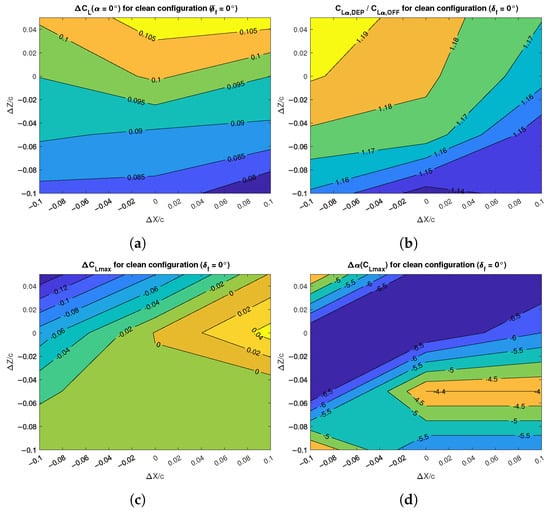
Figure 11.
Effects of DEP array positions on the lift characteristics of the clean wing: (a) lift increment; (b) lift gradient increment; (c) maximum lift increment; (d) stall angle change.
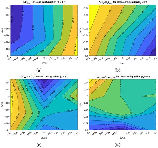
Figure 12.
Effects of DEP array positions on the drag and pitching moment characteristics of the clean wing: (a) minimum drag increment; (b) maximum aerodynamic efficiency change; (c) pitching moment increment; (d) pitching moment gradient change.
The lift coefficient at zero angle of attack increased when moving the propellers’ array upward, while there was no significant variation by moving it horizontally (Figure 11a). With respect to the unblown condition, the lift coefficient was increased by about 0.1, an increment that alone cannot justify the application of distributed propulsion. However, in this work, only the aero-propulsive effects are discussed, leaving design considerations elsewhere [24,25].
If the interest is in the linear range of the lift curve, the change in its slope is a good figure of merit. Here it is shown as the ratio between the values achieved in the propeller-on and propeller-off conditions. The blowing effect was such to increase the lift curve slope from 14% to 19%, with the maximum value achieved when the propellers’ array was located farther from the wing leading edge (Figure 11b).
The best position for the maximum lift coefficient was clearly the one closer to the wing leading edge and aligned with the wing chord plane, although the improvement with respect to the unblown condition was negligible (Figure 11c). Moving the propellers’ array ahead and above, the was reduced by about 0.15. One effect of enabling propeller blowing is the reduction of the angle of stall, which did not follow the same trend of the and varied from to with respect to the unblown condition (Figure 11d).
It is useful to evaluate the shift in minimum drag coefficient . The different configurations achieve such value at slightly different attitudes. Figure 12a shows that there was no net preference for propeller vertical location, while increased when getting closer to the wing. The increment was from 120 to 190 drag counts at the simulated Reynolds number of . To obtain the real impact of the aero-propulsive effects, the maximum aerodynamic efficiency must be observed (Figure 12b). The reduction of the lift-to-drag ratio by 4 to 6 points is apparent and, as stated above, was due to an increase of the induced drag. The closer and the lower was the propellers’ array with respect to the wing leading edge, the stronger was the reduction in aerodynamic efficiency.
The contour chart of Figure 12c shows that the change in pitching moment coefficient at zero angle of attack was between and . The position slightly below the baseline location acted as a saddle point, with the minimum values at the top and bottom positions and the maximum values at the positions closer and farther from the wing. Nevertheless, these shifts represent more than one-third of the propeller-off absolute value of the and they will certainly affect the trim condition, if such situation is replicated on a complete aircraft.
Finally, the change in pitching moment curve slope is shown as the ratio between propeller-on and propeller-off values in Figure 12d. The largest change was achieved with the propellers’ array located above the wing chord plane, where the value of the blown wing could be more than double the value of the unblown wing. This, together with the lift curve slope , defined a new position of the wing aerodynamic center. With respect to the reference point at , the aerodynamic center was found as:
Although the magnitude of the pitching moment derivative was significantly larger in prop-on conditions, the lift curve slope increased as well, such that the shift in wing aerodynamic center from the unblown to the blown condition was very small, vs. , respectively. This means that the wing stability contribution in pitch is not significantly affected by the distributed electric propulsion in cruise condition.
3.1.2. Local Effects of the Propellers on the Wing Aerodynamics
The spanwise section lift coefficient for two low angles of attack is shown in Figure 13, comparing unblown and blown conditions for all the propellers’ array positions. An illustration of the wing in front view is also given below the charts, where the vertical component of the air velocity is shown on the three disk planes (the actuator disks are shadowed). By looking at the charts and the illustration below them, the effects of propellers’ rotation are apparent. While the prop-off wing exhibited an almost elliptical lift distribution, the prop-on configurations were far from the optimal span loading. The reduction in lift-to-drag ratio is mainly attributed to the increase in induced drag because of the propellers’ slipstream. Propellers rotate inner-up, yielding to an increase of the local angle of attack—and section lift coefficient —in the region behind the left side of the disk (as seen in front view). Conversely, the wing regions behind the right side of the propeller disks were blown at a lower angle of attack. Thus, apart from an increase of the local lift coefficient due to the local flow speed increment, the inner-up rotation provided upwash and downwash on the inner and outer wing regions behind the disks, respectively. This also affected the wing root region, which was not blown by any propeller.
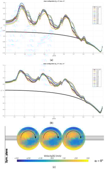
Figure 13.
Spanwise section lift distributions for the clean wing: (a) ; (b) ; (c) vertical velocity component in the disk plane.
The effects of wing finiteness are also visible on the spanwise lift distributions in blown condition. Despite the propellers working at the same rotational speed, the trend of the was to decrease along the wing span, as in the unblown condition. In addition, the spanwise change in behind each disk was not linear for all the propellers’ positions, but tended to form a sort of bulge on the right hand side for some of them, especially for the positions higher and farther from the wing leading edge. The area below these curves is larger than the others, as these positions provided a more effective blowing. This is in agreement with the values of the global lift coefficient and of the lift curve slope in Figure 11. In other words, higher and farther propeller positions are favorable for the clean wing at low angles of attack and this was confirmed by the section lift distribution.
The chordwise pressure coefficient is shown in Figure 14 for the same angles of attack. Two sections at the 75% radius around the middle disk are represented, on the inner and outer side, respectively. The chordwise pressure distribution on the inner section reveals the effect of both local flow speed and angle of attack increase: the whole curve inflated as well as the peak suction. This became more evident at higher angles of attack. The outer section was affected by the same phenomena, but the downwash due to the rotating propeller disk decreased the peak value, while the flow speed increment still inflated the plot on the rear part of the airfoil.
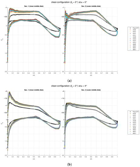
Figure 14.
Chordwise pressure distributions for the clean wing around the mid propeller: (a) ; (b) .
Again, the most effective blowing at low angles of attack, typical of cruise condition, was given by the propellers’ array located higher and farther from the wing leading edge, while on the opposite positions (lower and closer), less lift and drag were produced. In this regard, two scenes of the chordwise values of the skin friction coefficient for these two extreme positions are shown in Figure 15. Warmer colors indicate more friction, whereas white color indicates regions of incipient separated flow. Cooler colors indicate regions of recirculating flow because of the negative value of the skin friction coefficient. These regions were not visible on the upper wing surface at low angles of attack. The skin friction distributions show that the propellers’ blowing was a little more effective with the array located higher than the wing chord plane. The scenes also include a representation of propellers’ wake with the Q-criterion [47], which also highlights the effects of the propellers’ blowing.
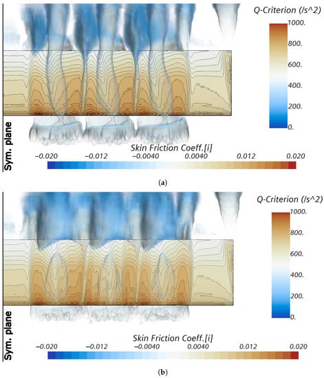
Figure 15.
Chordwise skin friction distributions for the clean wing: (a) configuration xFzU at ; (b) configuration xAzB at .
3.1.3. Effects of the Wing on the Propellers’ Performance
The virtual disk model of STAR-CCM+ enables the evaluation of the simplified propeller aerodynamics in a region surrounding the actuator disk. Although the propeller set point was assigned with the data of Table 6, the propeller coefficients were calculated with the data of Figure 9 from the assigned rotational rate and the surrounding flow field, which was altered by the bodies in proximity of the virtual disk. Figure 16 shows the variation of the advance ratio J, the thrust coefficient , the power coefficient , and the propeller efficiency with the angle of attack for the three propellers: DEP 1 is the inner disk, DEP 2 is the middle disk, and DEP 3 is the outer disk. Due to the effect of wing finiteness, the values achieved by the three propellers were slightly different, with the inner disk showing the largest variations.
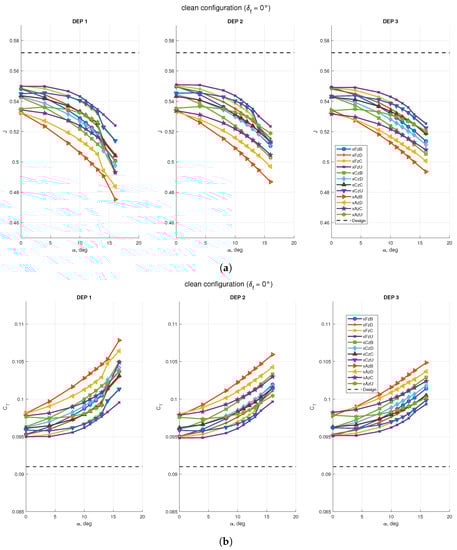
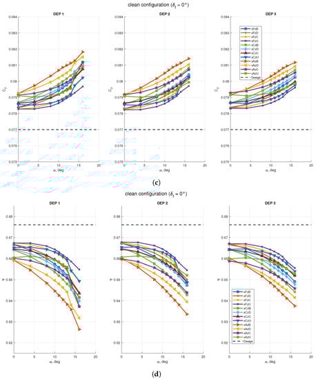
Figure 16.
Effects of the wing on propeller performance with STAR-CCM+ virtual disk model: (a) propellers advance ratio; (b) propellers’ thrust coefficient; (c) propellers’ power coefficient; (d) propellers’ efficiency. Design data is taken from Table 6, which are the assigned coefficients for the isolated propeller.
The value of the advance ratio J decreased with the angle of attack and remained below the design value for all the investigated positions. This is due to the combination of geometric angle of attack and wing-induced upwash . In fact, the inflow velocity—and consequently, the advance ratio J—should scale with , such that even at the propeller is working in non-axial flow. The lowest values were attained by the propeller at the bottom and closest position xAzB ( with respect to the baseline value at ), while the highest values were obtained at the top and farthest position xFzU ( with respect to the baseline value at ).
Conversely, thrust and power coefficients and increased with angle of attack and both values were always higher than the design condition. Again, the extreme positions of the propellers’ array showed the highest and lowest values, with the xAzB position varying from 8% to 20% and the xFzU position varying from 5% to 11% higher than the baseline value of , respectively. Thus, for the wing with flap retracted, the propeller position at bottom and closest to the leading edge was the most effective for its performance, the opposite of the effects of the propellers on the wing. Finally, the combination of advance ratio, thrust coefficient, and power coefficient was such to decrease the propellers’ efficiency up to 5% at high angle of attack. This highlights that propellers were not working in the design point evaluated for the isolated geometry. To keep them operating in the design point, RPM should be reduced to increase the advance ratio.
3.2. Flap in Take-Off Configuration
In this subsection, data about the effects of distributed propulsion on the wing with the flap deflected by are presented and discussed. Again, this subsection is divided into three parts concerning global effects of the propellers on the wing, local effects of the propellers on the wing, and the effects of the wing on the propeller aerodynamics, within the limits of the actuator disk model.
3.2.1. Global Effects of the Propellers on the Wing Aerodynamics
The effects of the propellers’ array on the wing aerodynamic coefficients are shown in Figure 17. As in the case of the clean wing, distributed propulsion increased the magnitude and the slope of the lift, drag, and pitching moment coefficients with respect to the angle of attack. Again, it can be observed that the distributed propulsion had the effect of an additional flap deflection.
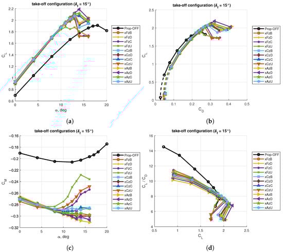
Figure 17.
Aerodynamic coefficients for the wing with flap deflected for take-off: (a) lift curves; (b) drag polars; (c) pitching moment curves; (d) aerodynamic efficiency curves.
As in the case of the clean wing, there were some propellers’ positions that made the wing stall earlier than other configurations, which achieved higher lift coefficients. The further increment in maximum lift coefficient due to the propellers operating with the flap deflected is useful, as this will further reduce the take-off distance for a given wing planform area (performance) or reduce the wing planform area for a given take-off distance (design) with respect to the unblown wing. However, in take-off it is equally important to keep a moderate increase in drag and pitching moment coefficients. Again, from the charts of Figure 17a,c, it was apparent that the differences in and at low angles of attack for the investigated propellers’ array positions were not significant as the shift from the unblown condition to any of the power-on configurations. This was not strictly true for the minimum drag coefficient (Figure 17b), where the difference of the values among the positions were comparable to the shift between prop-off and prop-on configurations.
However, from the trends of the lift-to-drag ratio in Figure 17d, it can observed that, at high values of the lift coefficient, say between 1.8 and 2.0, the difference between blown and unblown conditions became negligible, meaning that the wing with distributed propulsion was working with the same aerodynamic efficiency of the unblown wing. This was true also for the clean wing, but it is unlikely that it has to operate near the maximum lift coefficient. Conversely, the wing with flap deflected at take-off will operate between moderate and high angles of attack. It can also be observed that if the power-off configuration were made to stall at a higher lift coefficient, the aerodynamic efficiency of the blown wing would be higher than the prop-off value at that lift coefficient, as the slopes of the vs. curve indicate. Thus, at high angles of attack and beyond the maximum lift coefficient of the unblown wing, the configurations with the distributed propulsion become competitive in terms of aerodynamic efficiency at take-off.
To give a more accurate representation of the effects of the distributed propulsion on the wing with flap deflected at take-off, Figure 18 reports the variations of the lift capabilities with the propellers’ array positions in specific conditions. Similarly, the effects on the drag and pitching moment coefficients are shown in Figure 19.
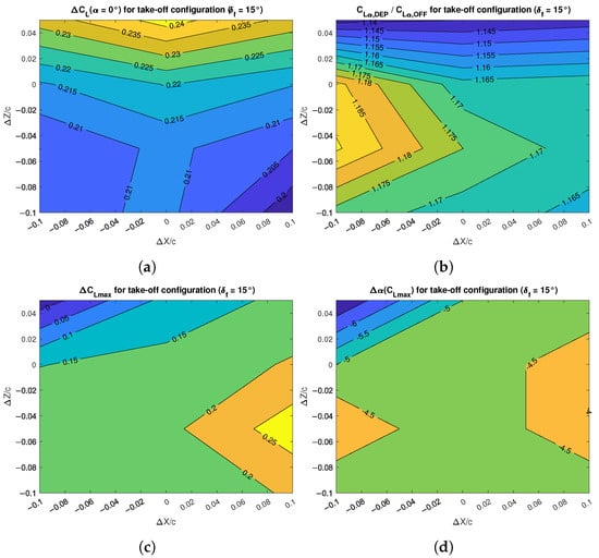
Figure 18.
Effects of DEP array positions on the lift characteristics of the wing with flap deflected for take-off: (a) lift increment; (b) lift gradient increment; (c) maximum lift increment; (d) stall angle change.
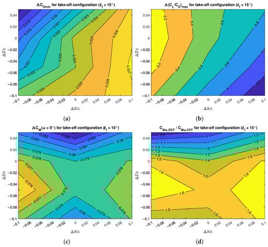
Figure 19.
Effects of DEP array positions on the drag and pitching moment characteristics of the wing with flap deflected for take-off: (a) minimum drag increment; (b) maximum aerodynamic efficiency change; (c) pitching moment increment; (d) pitching moment gradient change.
Figure 18a shows that the values of the lift coefficient at zero angle of attack achieved by the blown wing were very close each other, with the propellers’ array located on the top position performing best. Thus, the location of the distributed propellers was not relevant for the lift increment at very low angles of attack. However, Figure 18b shows that the values of the lift curve slope were sensibly different among the investigated positions, with a minimum increase of 14% with respect to the prop-off condition when the array was located on the highest position and a maximum increase of 19% when the array was located ahead and below the wing chord plane, with small differences with horizontal variations of the position.
The largest increment of the maximum lift coefficient was obtained with the propellers’ array located as close as possible to the wing leading edge and at 5% chord length below it (Figure 18c). The achieved increment of 0.25 was larger than the 0.10 value obtained in clean configuration, but it was still a non-disrupting result. The angle of stall was reduced by to , depending on the propellers’ positions (Figure 18d).
Figure 19a shows that the increase in minimum drag coefficient spanned about 100 drag counts at , with the maximum value achieved by the propellers located closer to the wing leading edge. There was a variation with the vertical position that became stronger as the horizontal distance to the leading edge increased. The difference in maximum aerodynamic efficiency was between about and for the prop-on condition as shown in Figure 19b, but this may be of some importance only in the initial phase of the take-off run, where the angle of attack is very low.
The pitching moment coefficient at zero angle of attack changed by about among the prop-on configurations (Figure 19c), but the skip between prop-off and prop-on conditions was almost two times larger, with the prop-off value being about and the prop-on value around . The pitching moment curve slope was practically unchanged for propellers located up and farther than the wing leading edge, but it was increased for propellers located below the wing chord plane, with a maximum increase of about 60% with respect to the unblown condition (Figure 19d). The maximum shift of the wing aerodynamic center, evaluated with Equation (6), was from in prop-off condition to in prop-on condition.
3.2.2. Local Effects of the Propellers on the Wing Aerodynamics
Here, the effects of distributed propulsion on the aerodynamic loads distribution at moderate angles of attack, specifically and , are discussed. In fact, if the interest is usually focused on the maximum lift coefficient achievable by the wing, it is also clear that not all the configurations share the same angle of stall. By assuming a safety speed between 1.1 and 1.2 of the take-off stall speed, a flapped wing with a maximum lift coefficient around 2.0 will operate at about , which roughly corresponds to for our configurations. This may also set the initial condition for the climb.
Figure 20 shows the spanwise section lift distribution for all the propellers’ array positions at the above cited angles of attack. The presence of the flap is apparent in both unblown and blown conditions, with the latter providing a significant local shift of . With the flap deflected at take-off, it seems that the least effective position for the lift enhancement at low-moderate angles of attack was the bottom one closer to the wing leading edge, as in the case of the clean wing. Conversely, there was no net prevalence of any position on the spanwise lift distribution, especially at , with the central positions performing slightly better.
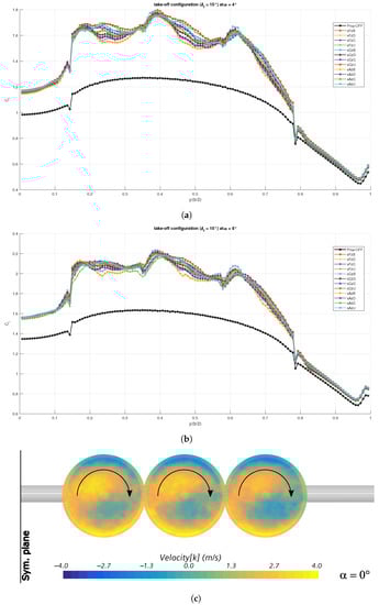
Figure 20.
Spanwise section lift distributions for the wing with flap deflected for take-off: (a) ; (b) ; (c) vertical velocity component in the disk plane.
Below the charts, there is a scene showing the variation of the vertical component of the velocity vector on the propellers’ disks, highlighting the direction of rotation. This scene is at with the only purpose of illustrating the flow field at the propellers’ disks. The larger and brighter regions indicate a mostly upwash flow due to the wing-induced circulation. At the top and bottom of these regions, just outside the propellers’ disks that are shadowed in the picture, there is downwash and upwash, respectively, due to the flow accelerating towards the virtual disks.
The behavior shown by the spanwise section lift distribution in Figure 20 is confirmed by the pressure coefficient distributions at the inner and outer 75% radius of the middle propeller in Figure 21. There was no significant change in at moderate angles of attack among the investigated propellers’ positions, with the bottom and closest one performing worse. As in the case of the clean wing, the pressure distribution was affected by both axial and tangential flow speed increments, with the inner section increasing both its peak value and the area enclosed by the curves, whereas the outer section increased only the rear upper portion of its value because of the propeller-induced downwash.
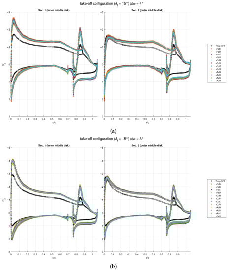
Figure 21.
Chordwise pressure distributions around the mid propeller for the wing with flap deflected for take-off: (a) ; (b) .
However, the upwash and downwash effects were consumed within the main wing component. The flap was unaffected by the propeller’s rotating slipstream, showing an increment of its peak value that was practically the same for both analyzed sections. In some cases, the peak value achieved by the flap was equal or even larger than that achieved by the main component. This, together with the interaction among propellers, should explain the flat spanwise trend in the section lift distribution shown in Figure 20.
Figure 22 shows the skin friction distribution on the upper wing surface at for the forward and central vertical position xFzC and the bottom rear position xAzB. As expected, there was no significant change between the two scenes, although the top figure indicates a more uniform blowing. The regions with white color were prone to flow separation. These were found near the trailing edge of the main component, as well as on a large part of the flap upper surface. Moreover, the areas between the propellers’ disks were not affected by the blowing effects. This was also true for the wing regions behind the propellers’ hub for the bottom array position. The Q-criterion shows the wake behind the propellers’ disks, especially at the inner (hub) and outer boundaries of the disks, and the wing trailing vortices.
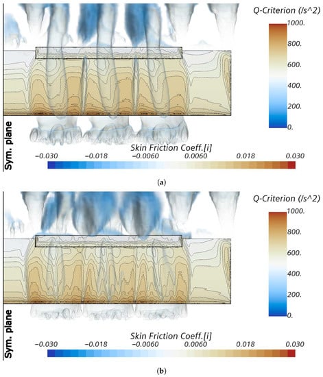
Figure 22.
Chordwise skin friction distributions for the wing with flap deflected for take-off: (a) configuration xFzC at ; (b) configuration xAzB at .
3.2.3. Effects of the Wing on the Propellers’ Performance
The effects of the wing with flap deflected at take-off on the distributed propellers’ performance are shown in Figure 23. As in the case of the clean wing, the advance ratio J and of the propeller efficiency were below the design values and decreased with the angle of attack for all the configurations. Conversely, the thrust and power coefficients, and , did increase with the angle of attack.
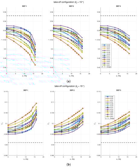
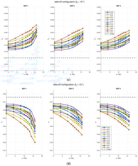
Figure 23.
Effects of the wing with flap deflected for take-off on propellers’ performance with STAR-CCM+ virtual disk model: (a) propellers’ advance ratio; (b) propellers’ thrust coefficient; (c) propellers power coefficient; (d) propellers’ efficiency. Design data are taken from Table 6, which are the assigned coefficients for the isolated propeller.
Among the three propellers, the innermost one showed the largest variations in performance with the angle of attack. The two configurations in which the propellers provided more and less thrust were xAzB and xFzU, respectively, indicating once again that the propeller had the largest performance enhancement where the wing was blown less effectively (xAzB position). In any case, the thrust coefficient was increased between the 5% and the 16% with respect to the data of the isolated propeller. Conversely, the advance ratio J was reduced between the 8% and the 18%, while the rotation rate of 7000 RPM was kept constant. Finally, the power coefficient increased as the thrust coefficient with a relatively smaller difference with respect to the design value. The combination of the propeller coefficients was such to decrease its efficiency from about 1% to 6%, with the largest loss at high angle of attack.
3.3. Flap in Landing Configuration
The effects of the distributed propulsion on the wing with flap deflected for landing are discussed in this subsection, which, as the previous parts, is divided into: global effects of the propellers on the wing, local effects of the propellers on the wing, and effects of the wing on the propellers.
3.3.1. Global Effects of the Propellers on the Wing Aerodynamics
The effects of the distributed propulsion on the aerodynamic coefficients are presented in Figure 24. These effects were stronger than those on the other flap configurations. On the lift coefficient , there was a net distinction of the values achieved by the different propellers’ array positions at high angles of attack (Figure 24a). In this case, there is a clear advantage in choosing a specific location for the propellers. Conversely, the curves with values at are not immediately distinguishable on this chart and will be discussed next on a contour plot. However, it appears that the configurations that stalled at a lower had a higher values of and that the curves with a higher slope did not achieve the highest .
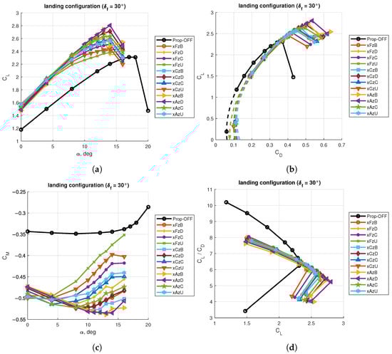
Figure 24.
Aerodynamic coefficients for the wing with flap deflected for landing: (a) lift curves; (b) drag polars; (c) pitching moment curves; (d) aerodynamic efficiency curves.
Similarly, the drag polar chart presents values of that were quite close each other at a given value of the (with the scale used in Figure 24b), with a clear distinction of the curves representing propellers’ positions that made the wing stall at higher values of the lift coefficient. The curves were also extrapolated to lower angles of attack to estimate the minimum drag coefficient with the modified parabolic drag formula of Equation (5).
Figure 24c shows several issues on the pitching moment evaluated at : the shift in from the unblown condition was much larger than the case of other flap deflections; there was a large variation of the pitching moment curve slope , where some curves exhibited a higher negative slope, i.e., a stronger pitch-down tendency, whereas others had a reverse sign, i.e., they had a pitch-up tendency; and the linearity of the pitching moment curves was lost approximately at the same angle of the lift curves.
Finally, the lift-to-drag ratio , which was not of a significant importance in landing conditions, is shown to highlight a smaller difference between prop-on and prop-off conditions with respect to other flap deflections (Figure 24d).
More details on the lift coefficient are given in Figure 25 and discussed here. The increment in lift coefficient at zero angle of attack was mostly dependent from the vertical position of the propellers’ array, achieving its maximum value of 0.4 at the top location (Figure 25a). Conversely, the maximum value of the was achieved with the propellers located at 5% chord length below the wing plane and as close as possible to the leading edge (Figure 25c). The attained increment of 0.45 in maximum lift coefficient was about twice that obtained with flap deflected at take-off. The angle of stall was reduced by about to and it seems that there was no correlation with the trends exhibited by the lift coefficient (Figure 25d). Finally, the lift curve slope, evaluated between , was increased by up to 30% and it was dependent from the vertical position of the propellers, with the lowest position achieving the maximum value (Figure 25b).
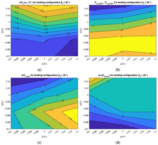
Figure 25.
Effects of DEP array positions on the lift characteristics of the wing with flap deflected for landing: (a) lift increment; (b) lift gradient increment; (c) maximum lift increment; (d) stall angle change.
Details on the drag and pitching moment coefficients are given in Figure 26. The extrapolated minimum drag coefficient is mostly function of the vertical position of the propellers, with the minimum value achieved at the top and farthest position from the wing leading edge (Figure 26a). Therefore, the maximum increase in was obtained with the propellers’ array located at the bottom positions.
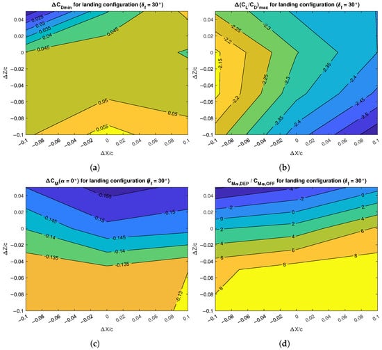
Figure 26.
Effects of DEP array positions on the drag and pitching moment characteristics of the wing with flap deflected for landing: (a) minimum drag increment; (b) maximum aerodynamic efficiency change; (c) pitching moment increment; (d) pitching moment gradient change.
Variations of the maximum lift-to-drag ratio are not critical in landing condition, but are shown in Figure 26b for completeness. As previously stated, there was a small loss in maximum aerodynamic efficiency within the range 2.1 to 2.4.
Similarly to the lift coefficient at zero angle of attack, the pitching moment coefficient at zero angle of attack achieved the maximum shift with respect to the unblown condition with the propellers’ array located on top, whereas the smallest increment was for the position at bottom and closest to the wing leading edge (Figure 26c). This is interesting, since the objective at landing is to maximize the lift coefficient without penalizing too much the pitching moment coefficient. The increments were from to , with an unblown value of about .
The pitching moment slope , evaluated between , presented a significant variation that was mainly a function of the vertical position of the propellers’ array (Figure 26d). With the reference point at , the bottom positions achieved a pitch-down tendency eight times stronger than the unblown wing, whereas the top positions had a significant pitch-up tendency. If this happens when designing an aircraft, it should be fixed in the preliminary design phase.
The variations of the wing of the aerodynamic center positions were significantly larger than those with other flap deflections. The for the prop-off wing was at , whereas the significant change in pitching moment curve slope together with a smaller variation of the lift curve slope determined a maximum shift of about , with the top and farthest array position achieving an value of and the bottom and closest array position moving the to .
3.3.2. Local Effects of the Propellers on the Wing Aerodynamics
The spanwise section lift distributions for all the propellers’ positions are shown in Figure 27 for and . The combined effect of distributed propulsion and flap deflection is apparent. At moderate and high angles of attack there was a clear distinction of the effect of the propellers’ array position, with the lowest and closest location performing best. Conversely, the highest and farthest position performed worst. Moreover, the positions providing more lift were those with a rather flat spanwise distribution of , very different to that generated on the clean wing at low angles of attack. A scene with the vertical velocity components on the propellers’ disks is shown below the charts. Even at , a large part of the flow field is affected by the upwash induced by the wing-flap combination.
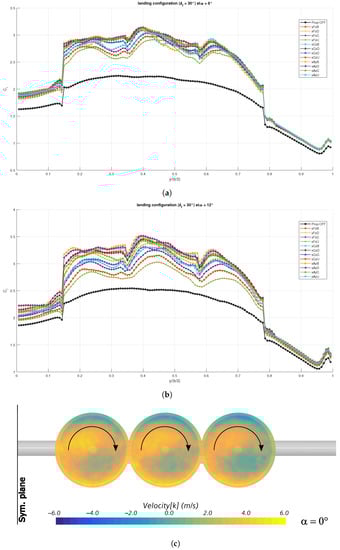
Figure 27.
Spanwise section lift distributions for the wing with flap deflected for landing: (a) ; (b) ; (c) vertical velocity component in the disk plane.
The chordwise pressure coefficient distributions are shown in Figure 28. The combined effects of axial and tangential propeller wake velocities were visible on both the inner section, showing an increase of both the peak and rear-end values, and the outer section, showing a reduction of the peak value and an increase of the rear-end value. The curve on the flap in prop-off condition reveals a flow separation that was not present in prop-on condition, further favoring the lift increment of the latter. Moreover, the peak values attained on the flap component were not dependent on the rotational slipstream, but only on the blowing effect, hence, on the position of the propellers. Again, these charts highlight that the most advantageous position for the distributed propulsion at high angles of attack was below the wing chord plane and as close as possible to the wing leading edge. Conversely, a higher and farther position provided the least increment in lift.
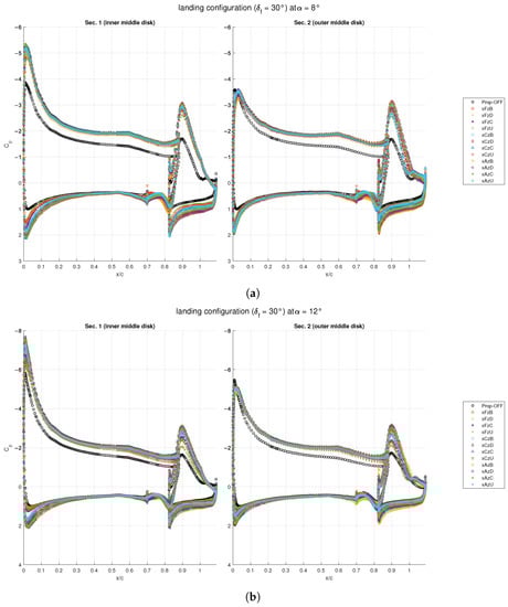
Figure 28.
Chordwise pressure distributions for the wing with flap deflected for landing: (a) ; (b) .
This is confirmed by the distribution of the skin friction coefficient shown in Figure 29 for . The configuration xFzU, although not being shadowed by the propellers’ hub, had the regions between the propellers’ wake unblown to some extent, as shown by the skin friction contour and the Q-criterion surfaces (Figure 29a). Moreover, the region behind the inner side of each propeller was blown less effectively. Conversely, the xAzD configuration showed a more uniform blowing behind both sides of the propellers, although it presented less friction in the regions behind the hub (Figure 29b). In addition, the regions of insufficient blowing between the wakes of the three disks were narrower than those of the other configuration. Finally, both scenes show that the propeller wakes were displaced towards the inner part of the wing, because of the cross-flow at high angle of attack.
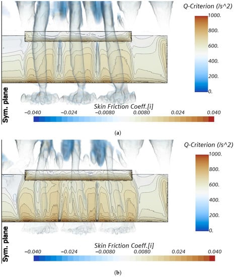
Figure 29.
Chordwise skin friction distributions for the wing with flap deflected for landing: (a) configuration xFzU at ; (b) configuration: xAzD at .
3.3.3. Effects of the Wing on the Propellers’ Performance
The trends reported in Figure 30 on the effects of the wing on the propellers’ performance are quite similar to those shown for the configurations with clean wing and flap deflected for takeoff. The values of the advance ratio J were always below the design value for the isolated propeller at 7000 RPM ( to , depending on the propellers’ positions), the values of the thrust coefficient were always above their design value ( to , depending on the propellers’ positions and angle of attack), and so were the values of the power coefficient ( to ). The combined effect was a reduction of the propellers’ efficiency with respect to the design value of the isolated propeller in axial flow, with an average reduction between 2% and 3% and the worst case achieving about efficiency loss at high angle of attack.
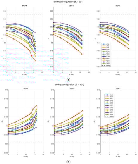
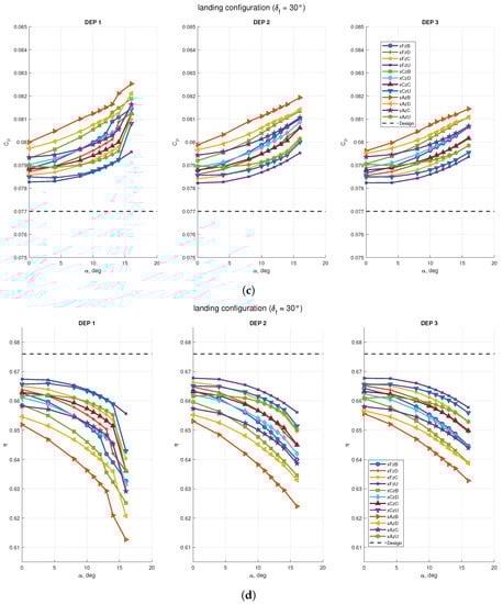
Figure 30.
Effects of the wing with flap deflected for landing on propellers’ performance with STAR-CCM+ virtual disk model: (a) propellers’ advance ratio; (b) propellers’ thrust coefficient; (c) propellers power coefficient; (d) propellers’ efficiency. Design data is taken from Table 6, which are the assigned coefficients for the isolated propeller.
Despite the blowing effect favored the propellers’ position close to the wing leading edge and lower than the wing’s chord plane xAzB, the circulation induced by the wing with flap was such to increase the value of the thrust coefficient with respect to the value of the isolated propeller for this position at all angles of attack, while the farthest and highest propellers’ array xFzU achieved the opposite performance, with a higher value of the advance ratio J and a lower value of the thrust coefficient . This was in contrast with the results of the previous sections, where the propellers’ thrust coefficients were higher where the wing was providing less maximum lift. With this last set of investigations, it seems that the effects of the wing on the propellers were not linked to the aerodynamic performance of the blown wing, but only to their relative positions.
It may be concluded that, in a given flap configuration and at a given angle of attack, the location of the distributed propellers’ array will affect both the aerodynamic coefficients of the wing and of the propellers, where the variations of the latter do not depend on the aerodynamic performance of the former, but only on the relative positions of the two items.
4. Conclusions
This paper has presented a numerical investigation on the aero-propulsive effects between three distributed propellers and a wing with flap with the aim to provide design guidelines for aerodynamic efficient fixed-wing UAVs. The simulations were performed to explore the effects of the propellers’ array location with respect to the wing leading edge and served as preliminary analyses to screen the most interesting positions for a wind tunnel test campaign. The wing had a straight, untwisted, and untapered planform to keep out the effects of section profile lofting and planform shape on the aerodynamic loading. A flap was added to investigate the effects of distributed propulsion in three different conditions: cruise, take-off, and landing. The propellers were simulated as actuator disks and without nacelle, since at the time of the numerical setup there were no detailed information on the propellers’ design.
The ratio between the propellers’ diameter and wing chord was reasonably adequate, according to previous investigations found in literature. However, the same literature lacked to indicate the effects of the propellers’ array position on the pitching moment, which is crucial for a fixed-wing aircraft equilibrium, stability, and control, as well as for the horizontal tail sizing. This work also attempted to fill this void of information.
The aero-propulsive effects have been classified into global, local, and wing-to-propeller. Global effects concern the influence of the propellers’ wake on the wing aerodynamic coefficients. Local effects deal with wing spanwise loading and chordwise pressure distributions affected by propellers’ slipstream, due to both axial and tangential flow acceleration. Wing-to-propeller effects refer to the wing-induced flow field on the propellers’ disks, which is different from the case of the isolated propeller.
Throughout the discussion on the results it appeared that the installation of an array of distributed propellers increased the magnitude of all the aerodynamic coefficients (lift, drag, and pitching moment) in different values according to the flap deflection, the angle of attack, and the propeller–wing relative position, in this order and for a given thrust level. The advantage of lift increment, which is the main objective of a high-lift distributed propellers’ array, may be shadowed by a significant increase in drag, especially in cruise condition (flap retracted). The numerical analyses highlighted that at low angles of attack the lift-to-drag ratio was reduced substantially with respect to the unblown condition. The maximum aerodynamic efficiency was reduced by a few units. However, at high angles of attack the lift-to-drag ratio in prop-on condition was comparable with that in prop-off condition. The blowing effect of the propellers permitted the wing to achieve a higher maximum lift coefficient without penalizing too much the aerodynamic efficiency, as was shown by the intersecting drag polars—prop-on vs. prop-off. At the same time, the angle of stall was slightly reduced, while the pitching moment coefficient became significantly more negative, highlighting how the propellers’ blowing was acting as an additional flap deflection. It is here remarked that all the aerodynamic coefficients were referred to the wing-flap system only, with the propulsive forces not considered for the lift generation. In other words, the interactions illustrated so far are relative to the propulsive indirect effects on the wing.
These observations were confirmed by the local effects, where numerical data have shown the influence of both propellers’ blowing and rotation on the spanwise wing loading as well as on the chordwise pressure distribution. For the former, the expected anti-symmetric load distribution induced on the wing by the propellers’ rotation had been mitigated by the interaction with the wing itself, highlighting the impact of the wing-propeller relative position, as well as of the angle of attack and flap deflection that strongly influenced the upwash. The spanwise loading was increased in the region interested by both the flap and the propellers’ slipstream, with a rather flat distribution for those positions that were more favorable to a higher maximum lift coefficient. Numerical data also clearly showed the effects of both axial and tangential velocities increments on the chordwise pressure distribution. The former acted as pure blowing, enlarging the area between the pressure coefficient curves of the upper and lower airfoil boundaries, while the latter provided upwash and downwash on the inner and outer sections of the wing around the mid propeller respectively, providing a further pressure expansion in the case of upwash and a reduction of the same peak in the case of downwash. Interestingly, the effects of the propellers’ rotating slipstream were exhausted on the wing main component, as both inner and outer flap sections showed the same expansion due to the blowing effect.
Finally, the effects of the wing on the propellers highlighted that the latter operated in off-design condition, with a reduced efficiency. This seems to be due to the wing-induced upwash at any angle of attack, altering the inflow velocity vector on the propeller’s disk. The absolute shift of propellers’ performance coefficients with respect to the design condition evaluated on the isolated propeller in axial flow depended on the angle of attack, flap deflection, and wing–propeller relative position. However, there was no dependence due to the change in the aerodynamic performance of the wing. The effects of the propellers’ positions, although not significantly different among them, highlighted that to get the maximum increase in lift coefficient at high angle of attack the distributed propellers’ array should be moved as close as possible to the wing leading edge and slightly below the wing chord’s plane. This was the position that favored high lift with the flap deflected for landing, but it was not the worst in terms of pitching moment coefficient as well as wing contribution to the aircraft longitudinal stability. At the same time, more lift meant certainly more drag, and this has to be taken into account if designing a wing with distributed propulsion for take-off.
Author Contributions
Conceptualization, D.C.; methodology, P.D.V. and D.C.; software, P.D.V.; validation, P.D.V. and D.C.; formal analysis, D.C.; investigation, V.O.; resources, F.N.; data curation, D.C.; writing—original draft preparation, D.C.; writing—review and editing, D.C. and P.D.V.; visualization, D.C.; supervision, P.D.V.; project administration, F.N.; funding acquisition, F.N. All authors have read and agreed to the published version of the manuscript.
Funding
This research was funded by the Italian PROSIB (Propulsione e Sistemi Ibridi per velivoli ad ala fissa e rotante—Hybrid Propulsion and Systems for fixed and rotary wing aircraft) project PNR 2015-2020 lead by Leonardo S.p.A.
Institutional Review Board Statement
Not applicable.
Informed Consent Statement
Not applicable.
Data Availability Statement
The authors confirm that the data supporting the findings of this study are available within the article.
Conflicts of Interest
The funders had no role in the design of the study; in the collection, analyses, or interpretation of data; in the writing of the manuscript; or in the decision to publish the results.
Abbreviations
The following abbreviations are used in this manuscript:
| Distributed Electric Propulsion | |
| Grid Convergence Index | |
| Leading Edge Asynchronous Propeller Technology | |
| Reynolds-averaged Navier-Stokes | |
| Revolutions Per Minute | |
| Unmanned Aerial Vehicle | |
| Vertical Take-Off and Landing | |
| Angle of attack | |
| Displacement or difference | |
| Deflection | |
| Upwash | |
| Propeller efficiency | |
| Taper ratio | |
| Free-stream flow density | |
| AR | Aspect ratio |
| b | Wing span |
| c | Wing chord |
| Wing | |
| Three-dimensional drag coefficient | |
| Three-dimensional minimum drag coefficient | |
| Two-dimensional drag coefficient | |
| Three-dimensional lift coefficient | |
| Three-dimensional lift curve slope | |
| Three-dimensional lift coefficient at zero angle of attack | |
| Three-dimensional maximum lift coefficient | |
| Two-dimensional lift coefficient | |
| Three-dimensional pitching moment coefficient | |
| Three-dimensional pitching moment curve slope | |
| Three-dimensional pitching moment coefficient at zero angle of attack | |
| Two-dimensional pitching moment coefficient | |
| Propeller power coefficient | |
| Pressure coefficient | |
| Propeller thrust coefficient | |
| D | Propeller diameter |
| k | Induced drag factor |
| P | Propeller power |
| T | Propeller thrust |
| J | Propeller advance ratio |
| N | Number of cells |
| n | Revolutions per second |
| Reynolds number | |
| S | Wing planform area |
| Free-stream flow speed | |
| X | Longitudinal position of the propeller array |
| x | Chordwise coordinate |
| Y | Lateral position of the propeller array |
| y | Spanwise coordinate |
| Non-dimensional wall distance | |
| Z | Vertical position of the propeller array |
| z | Vertical coordinate |
| Aerodynamic center | |
| Referred to DEP enabled (power-on condition) | |
| Flap | |
| Flap hinge | |
| Inner | |
| Referred to DEP disabled (power-off condition) | |
| Outer | |
| Root | |
| Reference point |
References
- Austin, R. Unmanned Aircraft Systems: UAVS Design, Development and Deployment; Aerospace Series; Wiley: Hoboken, NJ, USA, 2011. [Google Scholar]
- Marqués, P.; Da Ronch, A. Advanced UAV Aerodynamics, Flight Stability and Control: Novel Concepts, Theory and Applications; Aerospace Series; Wiley: Hoboken, NJ, USA, 2017. [Google Scholar]
- Ciliberti, D.; Della Vecchia, P.; Memmolo, V.; Nicolosi, F.; Wortmann, G.; Ricci, F. The Enabling Technologies for a Quasi-Zero Emissions Commuter Aircraft. Aerospace 2022, 9, 319. [Google Scholar] [CrossRef]
- Kim, H.D.; Perry, A.T.; Ansell, P.J. A Review of Distributed Electric Propulsion Concepts for Air Vehicle Technology. In Proceedings of the AIAA/IEEE Electric Aircraft Technologies Symposium, Cincinnati, OH, USA, 12–14 July 2018; American Institute of Aeronautics and Astronautics: Reston, VA, USA, 2018. [Google Scholar] [CrossRef]
- Schetz, J.A.; Hosder, S.; Dippold, V.; Walker, J. Propulsion and aerodynamic performance evaluation of jet-wing distributed propulsion. Aerosp. Sci. Technol. 2010, 14, 1–10. [Google Scholar] [CrossRef]
- Budziszewski, N.; Friedrichs, J. Modelling of a boundary layer ingesting propulsor. Energies 2018, 11, 708. [Google Scholar] [CrossRef]
- Rolt, A.; Whurr, J. Optimizing propulsive efficiency in aircraft with boundary layer ingesting distributed propulsion. In Proceedings of the International Symposium on Air Breathing Engines, Phoenix, AZ, USA, 25–30 October 2015. [Google Scholar]
- Valencia, E.; Alulema, V.; Rodriguez, D.; Laskaridis, P.; Roumeliotis, I. Novel fan configuration for distributed propulsion systems with boundary layer ingestion on an hybrid wing body airframe. Therm. Sci. Eng. Prog. 2020, 18, 100515. [Google Scholar] [CrossRef]
- Bevilaqua, P.; Yam, C. Propulsive efficiency of wake ingestion. J. Propuls. Power 2020, 36, 517–526. [Google Scholar] [CrossRef]
- Gnadt, A.R.; Isaacs, S.; Price, R.; Dethy, M.; Chappelle, C. Hybrid turbo-electric STOL aircraft for urban air mobility. In AIAA Scitech 2019 Forum, San Diego, CA, USA, 7–11 January 2019; American Institute of Aeronautics and Astronautics: Reston, VA, USA, 2019. [Google Scholar] [CrossRef]
- Straubinger, A.; Rothfeld, R.; Shamiyeh, M.; Büchter, K.D.; Kaiser, J.; Plötner, K.O. An overview of current research and developments in urban air mobility—Setting the scene for UAM introduction. J. Air Transp. Manag. 2020, 87, 101852. [Google Scholar] [CrossRef]
- Simmons, B.M.; Murphy, P.C. Aero-Propulsive Modeling for Tilt-Wing, Distributed Propulsion Aircraft Using Wind Tunnel Data. J. Aircr. 2022, 59, 1–17. [Google Scholar] [CrossRef]
- Bacchini, A.; Cestino, E. Electric VTOL configurations comparison. Aerospace 2019, 6, 26. [Google Scholar] [CrossRef]
- Nguyen Van, E.; Troillard, P.; Jézégou, J.; Alazard, D.; Pastor, P.; Döll, C. Reduction of Vertical Tail Using Differential Thrust: Influence on Flight Control and Certification. In Proceedings of the Advanced Aircraft Efficiency in a Global Air Transport System (AEGATS’18), Toulouse, France, 23–25 October 2018. [Google Scholar]
- Nguyen Van, E.; Alazard, D.; Pastor, P.; Döll, C. Towards an aircraft with reduced lateral static stability using electric differential thrust. In Proceedings of the 2018 Aviation Technology, Integration, and Operations Conference, Atlanta, GA, USA, 25–29 June 2018; American Institute of Aeronautics and Astronautics: Reston, VA, USA, 2018. [Google Scholar] [CrossRef]
- Nguyen Van, E.; Alazard, D.; Döll, C.; Pastor, P. Co-design of aircraft vertical tail and control laws using distributed electric propulsion. IFAC-PapersOnLine 2019, 52, 514–519. [Google Scholar] [CrossRef]
- Freeman, J.L.; Klunk, G.T. Dynamic Flight Simulation of Spanwise Distributed Electric Propulsion for Directional Control Authority. In Proceedings of the 2018 AIAA/IEEE Electric Aircraft Technologies Symposium, Cincinnati, OH, USA, 12–14 July 2018; American Institute of Aeronautics and Astronautics: Reston, VA, USA, 2018. [Google Scholar] [CrossRef]
- Patterson, M.D.; Borer, N.K.; German, B. A Simple Method for High-Lift Propeller Conceptual Design. In Proceedings of the 54th AIAA Aerospace Sciences Meeting, San Diego, CA, USA, 4–8 January 2016; American Institute of Aeronautics and Astronautics: Reston, VA, USA, 2016. [Google Scholar] [CrossRef]
- Moore, M.D. Misconceptions of Electric Aircraft and their Emerging Aviation Markets. In Proceedings of the 52nd Aerospace Sciences Meeting, National Harbor, MD, USA, 13–17 January 2014; American Institute of Aeronautics and Astronautics: Reston, VA, USA, 2014. [Google Scholar] [CrossRef]
- Stoll, A.M. Comparison of CFD and Experimental Results of the LEAPTech Distributed Electric Propulsion Blown Wing. In Proceedings of the 15th AIAA Aviation Technology, Integration, and Operations Conference, Dallas, TX, USA, 22–26 June 2015; American Institute of Aeronautics and Astronautics: Reston, VA, USA, 2015; pp. 22–26. [Google Scholar] [CrossRef]
- Deere, K.A.; Viken, S.A.; Carter, M.B.; Viken, J.K.; Derlaga, J.M.; Stoll, A.M. Comparison of High-Fidelity Computational Tools for Wing Design of a Distributed Electric Propulsion Aircraft. In Proceedings of the 35th AIAA Applied Aerodynamics Conference, Denver, CO, USA, 5–9 June 2017; American Institute of Aeronautics and Astronautics: Reston, VA, USA, 2017. [Google Scholar] [CrossRef]
- Della Vecchia, P.; Malgieri, D.; Nicolosi, F.; De Marco, A. Numerical analysis of propeller effects on wing aerodynamic: Tip mounted and distributed propulsion. Transp. Res. Procedia 2018, 29, 106–115. [Google Scholar] [CrossRef]
- Borer, N.K.; Patterson, M.D.; Viken, J.K.; Moore, M.D.; Bevirt, J.; Stoll, A.M.; Gibson, A.R. Design and Performance of the NASA SCEPTOR Distributed Electric Propulsion Flight Demonstrator. In Proceedings of the 16th AIAA Aviation Technology, Integration, and Operations Conference, Washington, DC, USA, 13–17 June 2016; American Institute of Aeronautics and Astronautics: Reston, VA, USA, 2016. [Google Scholar] [CrossRef]
- Orefice, F.; Della Vecchia, P.; Ciliberti, D.; Nicolosi, F. Correction: Aircraft Conceptual Design Including Powertrain System Architecture and Distributed Propulsion. In Proceedings of the AIAA Propulsion and Energy Forum, Indianapolis, IN, USA, 19–22 August 2019; American Institute of Aeronautics and Astronautics: Reston, VA, USA, 2019. [Google Scholar] [CrossRef]
- Orefice, F.; Della Vecchia, P.; Ciliberti, D.; Nicolosi, F. Preliminary Design to Fulfil Future Market Demand of Electric Aircraft. Int. Rev. Aerosp. Eng. (IREASE) 2021, 14, 294. [Google Scholar] [CrossRef]
- Poggi, C.; Rossetti, M.; Bernardini, G.; Iemma, U.; Andolfi, C.; Milano, C.; Gennaretti, M. Surrogate models for predicting noise emission and aerodynamic performance of propellers. Aerosp. Sci. Technol. 2022, 125, 107016. [Google Scholar] [CrossRef]
- de Vries, R.; van Arnhem, N.; Sinnige, T.; Vos, R.; Veldhuis, L.L. Aerodynamic interaction between propellers of a distributed-propulsion system in forward flight. Aerosp. Sci. Technol. 2021, 118, 107009. [Google Scholar] [CrossRef]
- Keller, D. Towards higher aerodynamic efficiency of propeller-driven aircraft with distributed propulsion. CEAS Aeronaut. J. 2021, 12, 777–791. [Google Scholar] [CrossRef]
- Wang, K.; Zhou, Z.; Zhu, X.; Xu, X. Aerodynamic design of multi-propeller/wing integration at low Reynolds numbers. Aerosp. Sci. Technol. 2019, 84, 1–17. [Google Scholar] [CrossRef]
- Xue, C.; Zhou, Z. Inverse aerodynamic design for DEP propeller based on desired propeller slipstream. Aerosp. Sci. Technol. 2020, 102, 105820. [Google Scholar] [CrossRef]
- Gentry, G.L.J.; Takallu, M.A.; Applin, Z.T. Aerodynamic Characteristics of a Propeller-Powered High-Lift Semispan Wing; Technical Report NASA TM-4541; NASA: Washington, DC, USA, 1994.
- Fei, X.; German, B.; Patterson, M.D. Exploring the Effects of Installation Geometry in High-Lift Propeller Systems. In Proceedings of the 2018 AIAA Aerospace Sciences Meeting, Kissimmee, FL, USA, 8–12 January 2018; American Institute of Aeronautics and Astronautics: Reston, VA, USA, 2018. [Google Scholar] [CrossRef]
- Serrano, J.R.; Tiseira, A.O.; García-Cuevas, L.M.; Varela, P. Computational Study of the Propeller Position Effects in Wing-Mounted, Distributed Electric Propulsion with Boundary Layer Ingestion in a 25 kg Remotely Piloted Aircraft. Drones 2021, 5, 56. [Google Scholar] [CrossRef]
- Serrano, J.R.; García-Cuevas, L.M.; Bares, P.; Varela, P. Propeller Position Effects over the Pressure and Friction Coefficients over the Wing of an UAV with Distributed Electric Propulsion: A Proper Orthogonal Decomposition Analysis. Drones 2022, 6, 38. [Google Scholar] [CrossRef]
- de Rosa, D.; Morales Tirado, E.; Mingione, G. Parametric Investigation of a Distributed Propulsion System on a Regional Aircraft. Aerospace 2022, 9, 176. [Google Scholar] [CrossRef]
- McGhee, R.J.; Beasley, W.D. Effects of Thickness on the Aerodynamic Characteristics of an Initial Low-Speed Family of Airfoils for General Aviation Applications; Technical Report NASA TM X-72843; NASA: Washington, DC, USA, 1976.
- Viken, J.K.; Viken, S.; Deere, K.A.; Carter, M. Design of the Cruise and Flap Airfoil for the X-57 Maxwell Distributed Electric Propulsion Aircraft. In Proceedings of the 35th AIAA Applied Aerodynamics Conference, Denver, CO, USA, 5–9 June 2017; American Institute of Aeronautics and Astronautics: Reston, VA, USA, 2017. [Google Scholar] [CrossRef]
- Spalart, P.R.; Allmaras, S.R. A one equation turbulence model for aerodynamic flows. AIAA J. 1992, 94, 439. [Google Scholar]
- Spalart, P.R.; Rumsey, C.L. Effective Inflow Conditions for Turbulence Models in Aerodynamic Calculations. AIAA J. 2007, 45, 2544–2553. [Google Scholar] [CrossRef]
- Celik, I.B.; Ghia, U.; Roache, P.J.; Freitas, C.J.; Coleman, H. Procedure for Estimation and Reporting of Uncertainty Due to Discretization in CFD Applications. J. Fluids Eng. 2008, 130, 078001. [Google Scholar] [CrossRef]
- Siemens Digital Industries Software. STAR-CCM+ 2020.2.1 User Manual; Siemens PLM Software: Plano, TX, USA, 2020. [Google Scholar]
- Drela, M. XROTOR. Available online: https://web.mit.edu/drela/Public/web/xrotor/ (accessed on 23 March 2022).
- Drela, M. XFOIL. Available online: https://web.mit.edu/drela/Public/web/xfoil/ (accessed on 30 December 2022).
- Klein, P.C. Parametric Modeling and Optimization of Advanced Propellers for Next-Generation Aircraft. PhD Thesis, Delft University of Technology, Delft, The Nethlands, 2017. [Google Scholar]
- Bergmann, O.; Goetten, F.; Braun, C.; Janser, F. Comparison and Evaluation of Blade Element Methods Against RANS Simulations and Test Data. In Proceedings of the Deutscher Luft- und Raumfahrtkongress—DLRK 2020, Virtual Meeting, 1–3 September 2020; Deutsche Gesellschaft für Luft- und Raumfahrt—Lilienthal-Oberth e.V.: Bonn, Germany, 2020. [Google Scholar]
- Ciliberti, D.; Nicolosi, F. Design, Analysis, and Testing of a Scaled Propeller for an Innovative Regional Turboprop Aircraft. Aerospace 2022, 9, 264. [Google Scholar] [CrossRef]
- Jeong, J.; Hussain, F. On the identification of a vortex. J. Fluid Mech. 1995, 285, 69–94. [Google Scholar] [CrossRef]
Disclaimer/Publisher’s Note: The statements, opinions and data contained in all publications are solely those of the individual author(s) and contributor(s) and not of MDPI and/or the editor(s). MDPI and/or the editor(s) disclaim responsibility for any injury to people or property resulting from any ideas, methods, instructions or products referred to in the content. |
© 2023 by the authors. Licensee MDPI, Basel, Switzerland. This article is an open access article distributed under the terms and conditions of the Creative Commons Attribution (CC BY) license (https://creativecommons.org/licenses/by/4.0/).