Improved Dyna-Q: A Reinforcement Learning Method Focused via Heuristic Graph for AGV Path Planning in Dynamic Environments

Abstract

Dyna-Q is a reinforcement learning method widely used in AGV path planning. However, in large complex dynamic environments, due to the sparse reward function of Dyna-Q and the large searching space, this method has the problems of low search efficiency, slow convergence speed, and even inability to converge, which seriously reduces the performance and practicability of it. To solve these problems, this paper proposes an Improved Dyna-Q algorithm for AGV path planning in large complex dynamic environments. First, to solve the problem of the large search space, this paper proposes a global path guidance mechanism based on heuristic graph, which can effectively reduce the path search space and, thus, improve the efficiency of obtaining the optimal path. Second, to solve the problem of the sparse reward function in Dyna-Q, this paper proposes a novel dynamic reward function and an action selection method based on the heuristic graph, which can provide more intensive feedback and more efficient action decision for AGV path planning, effectively improving the convergence of the algorithm. We evaluated our approach in scenarios with static obstacles and dynamic obstacles. The experimental results show that the proposed algorithm can obtain better paths more efficiently than other reinforcement-learning-based methods including the classical Q-Learning and the Dyna-Q algorithms.

1. Introduction

The automated guided vehicle (AGV) is widely used for material transport tasks in manufacturing workshops due to its efficient transportation mode. As an essential part of the manufacturing workshop, AGV has played an indispensable role [1,2]. Path planning is the central key in the field of AGV research. It calculates the feasible path from the starting position to the goal position in the map, and ensures that AGV will not collide with static and dynamic obstacles in the moving process. How to achieve collision-free and conflict-free efficient paths for AGVs in dynamic environments is still one of the main focuses of AGV system research.

Many researchers have used many representative algorithms to solve the path planning problem of AGV, including graph-based search algorithms such as Dijkstra [3], A* [4,5], D* [6], etc. These algorithms have the advantage of being simple and easy to implement and have been widely used in AGV path planning. However, when the environment is large and the obstacles are complex, the state space grows exponentially and the time efficiency of the algorithm is low. Aiming at the above problems, many algorithms have been proposed, such as Rapidly exploring Random Trees and intelligent bionic algorithms. Rapidly exploring Random Trees (RRT) [7] is a sampling-based path planning algorithm to solve the path planning problem of AGV. Its advantages are high efficiency and speed in high-dimensional path search, while the disadvantages are that these algorithms usually conduct random search in the sampling environment to find the path and the results are often not optimal. Intelligent bionic algorithms are discovered through bionic research. Typical algorithms include the genetic algorithm (GA) [8,9], ant colony algorithm (ACA) [10], and particle swarm optimization (PSO) [11]. When dealing with the path planning problem under the complex dynamic environment information, the inspiration from nature often works well. However, in the complex map environment, there are still some problems, such as slow calculation speed and easy falling into local optimum.

Almasri et al. [12] proposed a route following and obstacle avoidance technology relying on low-cost infrared sensors, which can be easily used in real-time control applications of microcontrollers. Matveev et al. [13] proposed an integrated navigation strategy to safely guide the robot to reach the target through an environment full of mobile non-convex obstacles. Tanveer et al. [14] defined the path to be followed as a curve on the plane and fed it back to the path tracking controller. Obstacles generated the final safe path by modifying the Gaussian function modeling of the original function. This method has strong robustness and security. These three methods can quickly obtain a feasible path and avoid obstacles; however, the path obtained by these methods may be suboptimal.

In recent years, with the rapid development of deep learning (DL) and reinforcement learning (RL), the applications of RL have achieved significant breakthroughs in many fields, such as games [15,16], healthcare [17], robotics [18], etc. Reinforcement learning is an artificial intelligence method, which emphasizes that agents adapt to complex environments by constantly interacting with the environment to learn the best strategies. RL can actively learn and has the characteristics of adapting to complex dynamic environments. RL technology provides a new way to solve path planning problems. More and more scholars have introduced learning-based methods into the field of path planning [19,20] to solve the limitations of classical path planning methods.

RL algorithms can be classified into model-free reinforcement learning and model-based reinforcement learning according to whether there is an environment model or not. Model-free reinforcement learning algorithm directly improves the policy or estimates the value function according to the data sampled by agents and environment interaction, such as classical Q-Learning [21], Sarsa, and other temporal-difference algorithms. Among them, the Q-Learning algorithm is widely used in path planning problems [19,22,23] because of its advantages of learning and no need for environmental maps. Many researchers apply Euclidean distance to the calculation of fitness function and reward function of Q-Learning. For example, the Euclidean distance between the current position of the mobile robot and the target position is used to evaluate the fitness function of the multiple mobile robots environment [24]. Low et al. [25] added distance measurement to Q-Learning to guide agents to move toward the target position.

With the increasing complexity of the map environment, the Q-Learning algorithm shows the characteristics of low learning efficiency and slow convergence. Dyna-Q [26] is a classical model-based reinforcement learning algorithm that integrates planning and direct RL methods. The direct RL method is to improve the value function and policy by using the real experience generated by agent interaction with the environment. At the same time, the algorithm also learns an environment model and then uses this model to assist agents in policy promotion or value estimation; so, Dyna-Q has high efficiency. Viet et al. [27] evaluated the efficiency of five reinforcement learning algorithms in path planning, including Q-Learning, Sarsa, Q($\lambda$), Sarsa($\lambda$), and Dyna Q. The experimental results show that Dyna-Q has a faster convergence speed in solving the path planning problem of mobile robots.

In order to further improve the convergence performance of Dyna-Q, a common way to improve the Dyna-Q algorithm is to combine Dyna-Q with other algorithms. An Improved Dyna-H algorithm was proposed in [28]. In the planning process of the Dyna-Q algorithm, those actions that lead to the worst trajectory were taken to simulate the update policy, integrating the advantages of heuristic search into Dyna agents. Dabouni et al. [29] proposed a direct heuristic dynamic programming algorithm based on dynamic programming (Dyna HDP). By combining neural networks and Dyna, the optimal policy efficiency can be improved in the least number of experiments. Pei et al. [30] proposed a method incorporating the $ϵ-greedy$ policy, which is a new action selection policy, combined with simulated annealing mechanism. This policy combines heuristic reward function and heuristic action to solve the exploration utilization dilemma and improve the convergence and learning efficiency of path planning.

Wang et al. [31] introduced an exploration factor that applies the technology of ant colony algorithm to the selection of candidates in indirect learning. A hybrid exploration strategy is proposed to improve the sample efficiency of the Dyna-Q algorithm. Zajdel [32] proposed a epoch-incremental learning method, which uses breadth-first search to determine the shortest distances between the non-terminal states observed and the target state in each episode, and performs additional policy updates based on these distances.

Although Dyna-Q has shown excellent performance in path planning, there are still some difficulties and challenges in path planning in large dynamic environments. First of all, when the map environment is large, the sparse reward problem makes it difficult for AGV to explore the target location, which leads to many iterations and low learning efficiency. Improving the search efficiency and convergence speed of the Dyna-Q algorithm is still a challenge. The second is how to plan a collision-free and efficient path in an environment with multiple dynamic obstacles.

In order to solve the above difficulties, this research proposes an Improved Dyna-Q algorithm for path planning in dynamic environments. Different from the Dyna-Q algorithm, the Improved Dyna-Q algorithm adopts a novel global guidance mechanism based on heuristic graph, and combines an improved dynamic reward function and an improved heuristic planning strategy. The global guidance mechanism guides AGV to move towards the target position for a long time but does not require AGV to strictly follow the global guidance mechanism. The advantage is that AGV is encouraged to explore all potential solutions to avoid falling into the locally optimal solution.

The Improved Dyna-Q algorithm proposed in this study is applied to solve the AGV path planning in a dynamic environment with the following main contributions:

• Propose a global path guidance mechanism based on heuristic graph for large complex dynamic environments to effectively reduce the path search space and improve the efficiency of the algorithm in searching for the optimal path.
• Propose a new dynamic reward function and action selection method, which can provide more intensive feedback signals and more efficient action selection for AGV path planning, so as to effectively solve the problem that the algorithm converges slowly due to the sparse Dyna-Q rewards.
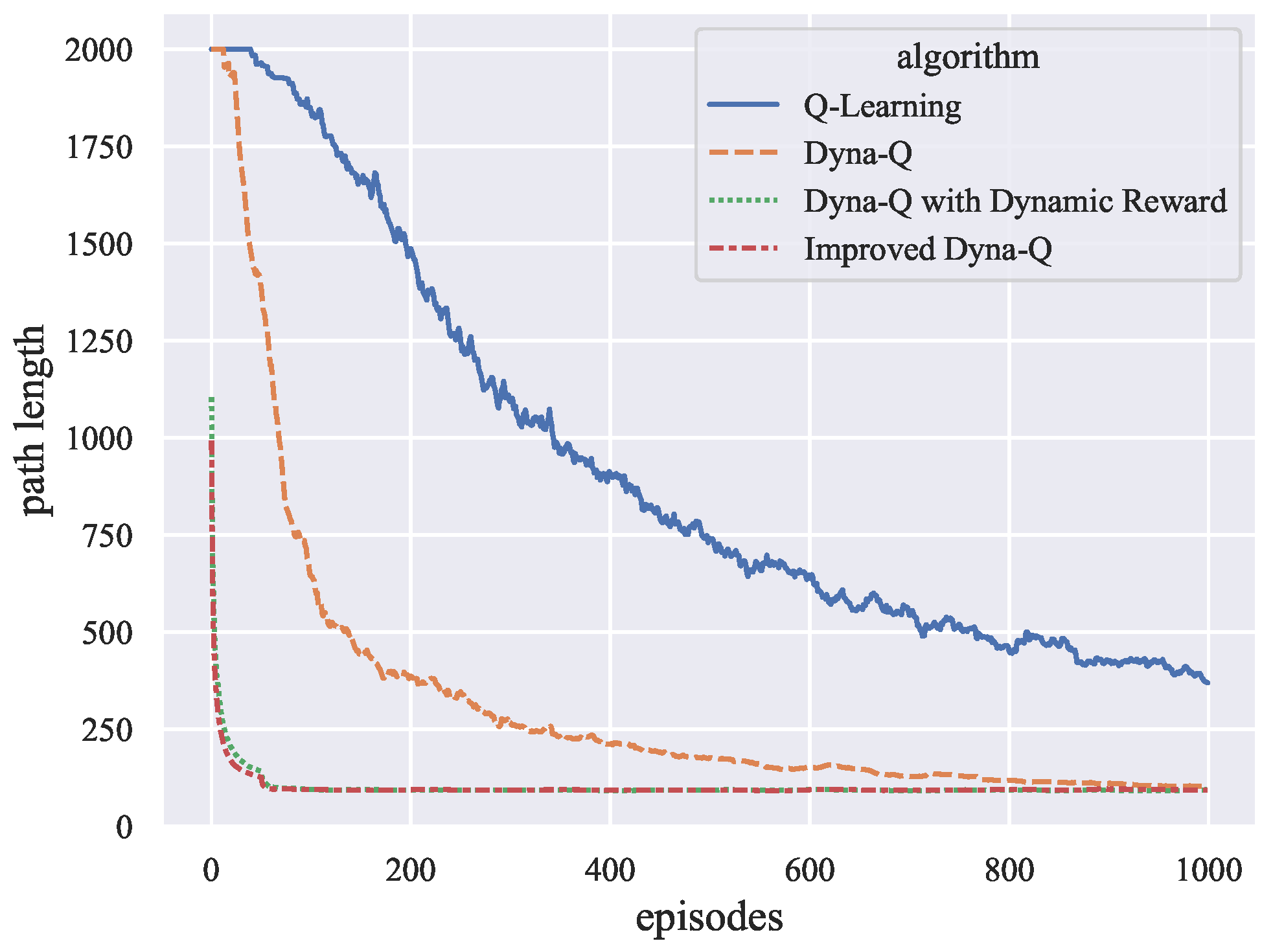
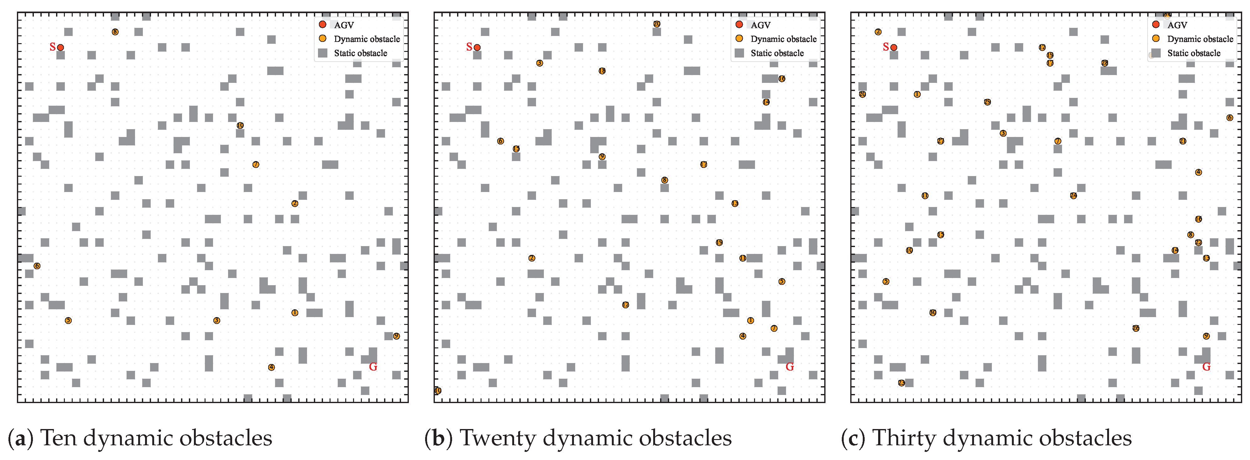
• The experimental results on random obstacle maps and maps with different numbers of dynamic obstacles show that the proposed algorithm has the advantage of fast convergence in unknown static environments; moreover, it can effectively solve the problem of AGV path planning in the environment of the different number of dynamic obstacles, without obtaining or predicting the trajectory of dynamic obstacles.

The rest of this paper is arranged as follows: Section 2 introduces the relevant background, including the path planning problem in dynamic environments, and the basic concepts of reinforcement learning and the Dyna-Q algorithm. In Section 3, we discuss the details of the proposed algorithm and describe the concept of heuristic graph in detail. In Section 4, we discuss simulation experiments and verify the efficiency of our method through some comparative experiments. Finally, Section 5 summarizes the work of this paper.

2. Related Background

Reinforcement learning is used to learn how to optimize goals by interacting with the environment through trial and error. The theoretical framework of RL is usually based on a Markov Decision Process (MDP). In this section, we first describe the AGV path planning problem in dynamic environments; then, we briefly summarize the theory of RL and MDP, and finally introduce the Dyna-Q algorithm.

2.1. Problem Description

This work considers an undirected grid graph environment $G(V,E)$ with size $W\times H$, where V is a set of vertices of the graph G, $V\subseteq \left\{\right(i,j)\mid 1\le i\le W,1\le j\le H\}$. The length of each grid is L, and E is the edge of the graph G. The set of $N_s$ static obstacles in the environment is defined as $V_s=\{s_1,\dots ,s_{N_s}\}$, $s_i\subset V$, $s_i$ represents each static obstacle vertex, and $N_s$ is the total number of static obstacles. The set of free cells excluding static obstacles is defined as $V_f=V\backslash V_s$. Following the traditional 4-way connectivity rule, for each vertex $v=(i,j)\in V$, its neighborhood is $N\left(v\right)=\{(i-1,j),(i+1,j),(i,j-1),(i,j+1)\}\cap V_f$. The set of dynamic obstacles $V_d\left(t\right)=\{d_1\left(t\right),\dots ,d_{N_d}\left(t\right)\}$ denotes the position of $N_d$ dynamic obstacles at time t, where $d_i\left(t\right)=(i,j)\in V_f$.

Definition 1. 

(Path $\mathcal{P}$)   For an AGV $\mathcal{A}$ with the start position $\alpha \in V_f$ and the goal position $\beta \in V_f,\beta \ne \alpha$, where $V_f$ is the set of free cells, a path is defined as a sequence of $T+1$ vertices $\mathcal{P}=(p_0,\dots ,p_T)$ satisfying (i) $p_0=\alpha$; (ii) $p_T=\beta$; (iii) $\forall 1\le t\le T,p_{t-1}=p_t$ or $p_{t-1}\in N\left(p_t\right)$, where $p_t$ denotes the path node of a time step t.

Definition 2. 

(A conflict-free path $\mathcal{P}$)   For a path $\mathcal{P}$ to be conflict-free, $\forall 1\le t\le T,p_t\in \mathcal{P}$, where $p_t$ denotes the path node of each time step t, it must satisfy (i) $p_t\notin V_s$, where $V_s$ is the set of static obstacles (no collision with static obstacles); (ii) $p_t\notin V_d\left(t\right)$, where $V_d\left(t\right)$ is the set of position of dynamic obstacles at time step t (no vertex conflict with all dynamic obstacles); (iii) $\forall 0\le i\le N_d,(p_{t-1},p_t)\ne (d_i\left(t\right),d_i(t-1))$, where $p_t$ is the path node at time step t and $d_i\left(t\right)$ is the position of the ith dynamic obstacle at time step t (no edge conflict with all dynamic obstacles).

The AGV path planning problem can be expressed as an optimization problem. The optimization objective includes an objective function that minimizes the path length of AGV from the starting position to the target position and avoids the constraint of collision with static or dynamic obstacles on the path.

Since obstacles are usually irregular in shape, if a grid contains any obstacle area, the entire grid is considered as an obstacle grid. Dynamic obstacles can move randomly at the vertices of graph G. We consider a similar scenario in [33], where a camera is installed at the top of the AGV workspace to capture dynamic obstacle information. This paper assumes that the AGV can obtain its global position in the environment in the process of AGV movement. This paper assumes that the AGV knows the information of all static obstacles. However, this paper does not assume that the AGV knows the trajectory of dynamic obstacles. AGV can only obtain the current position of dynamic obstacles within its local field of vision.

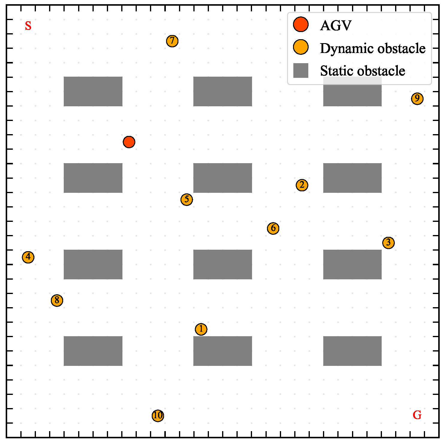
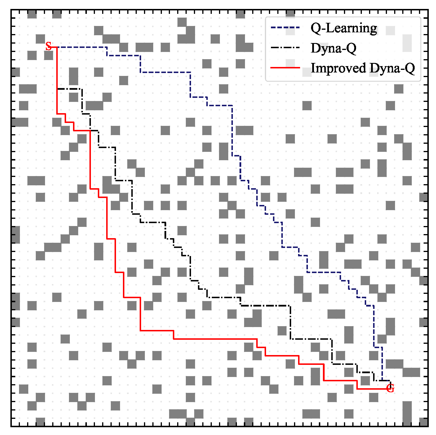
Specifically, to illustrate the AGV path planning problem in this study, Figure 1 shows an example of AGV path planning in a dynamic environment.

2.2. MDP of AGV Path Planning

Standard reinforcement learning is a learning process through trial-and-error interaction with the environment in a Markov Decision Process framework. In general, an MDP is represented as a five-tuple $M=\{S,A,P,R,\gamma \}$, where S is a set of environmental states $s\in S$, A is a set of agent actions $a\in A$, P is a transition probability function between states, R is a reward function, and $\gamma$ is a discount rate $0\le \gamma \le 1$. RL agent takes an action $a_t\in A$ in some state $s_t\in S$. The state of environment is transferred to $s_{t+1}\in S$, and a reward $r_{t+1}$ is given. The agent continuously learns by interacting with the environment and eventually learns an optimal policy to reach the goal.

Definition 3. 

(State set S)   In this work, the map environment is modeled as a grid map; so, the state set S is defined as

$$S=\{s=(x,y)\mid 1\le x\le W,1\le y\le H\}$$

(1)

where W and H are the width and height of the grid map.

Definition 4. 

(Action set A)   The action set is the set of all possible actions of an AGV to move from the current state to the next state. The action set of the AGV is defined as $A=\{a_0,a_1,a_2,a_3,a_4\}$ in this study, which, respectively, denote waiting for a time in the current state, forward, backward, left, right.

Definition 5. 

(Reward function R)   The typical reward function R is assigned as

$$R(s,a)=\left\{\begin{array}{c}{r}_1,s^{\prime }\in Goal\hfill \\ r_2,s^{\prime }\in V_o\cup V_d\hfill \\ 0,otherwise\hfill \end{array}\right.$$

(2)

The typical reward function gives a positive reward $r_1>0$ when the AGV reaches the target position, a negative reward $r_2<0$ when it collides with a static or dynamic obstacle, and a reward value of 0 in other cases.

Given the MDP definition, the reinforcement learning objective is to learn an optimal policy that maximizes the expected sum of future rewards [34]. Policy $\pi$ is a mapping from states to probabilities of selecting each possible action. The discounted return $G_t$ is defined by

$$G_t=r_{t+1}+\gamma r_{t+2}+{\gamma }^2{r}_{t+3}+\cdots =\sum _{k=0}^{\infty }{\gamma }^k{r}_{t+k+1},\gamma \in [0,1]$$

(3)

where $r_t$ denotes the immediate reward at time t and $\gamma$ is a discount factor indicating the magnitude of the effect of future rewards on the present. Therefore, the reinforcement learning objective can be expressed as follows [35]:

$$J\left(\pi \right)=\underset{\pi }{max}\mathbb{E}\left[G_t\right]=\underset{\pi }{max}{\mathbb{E}}_{\tau \sim \pi }[\sum _{t=1}^{T}r(s_t,a_t)]$$

(4)

In Equation (4), T is the time step at the end of each episode and $\tau$ is the episode trajectory (the sequence of observations and actions obtained throughout the episode). The goal is to learn an optimal policy ${\pi }^{*}$, which maximizes the expected sum of future reward.

2.3. Dyna-Q Algorithm

Q-Learning is a classical model-free RL algorithm for solving MDP, whose main advantage is the utilization of a temporal-difference algorithm to achieve off-policy learning.

Definition 6. 

(Q-value $Q(s,a)$)   $Q_{\pi }(s,a)$ is defined by the expected return of the state-action pair $(s,a)$ under the policy π. The equation is as follows:

$$\begin{array}{cc}\hfill Q_{\pi }(s,a)& ={\mathbb{E}}_{\pi }[G_t\mid s_t=s,a_t=a]\hfill \\ \hfill & ={\mathbb{E}}_{\pi }[\sum _{k=0}^{\infty }{\gamma }^k{r}_{t+k+1}\mid s_t=s,a_t=a]\hfill \end{array}$$

(5)

The core idea of the Q-Learning algorithm is that the Q-value of the next state–action pair is generated by the policy to be evaluated rather than the Q-value of the next state–action pair that follows the present policy. The final policy of Q-Learning is obtained by iterating the state–action value function $Q(s,a)$.

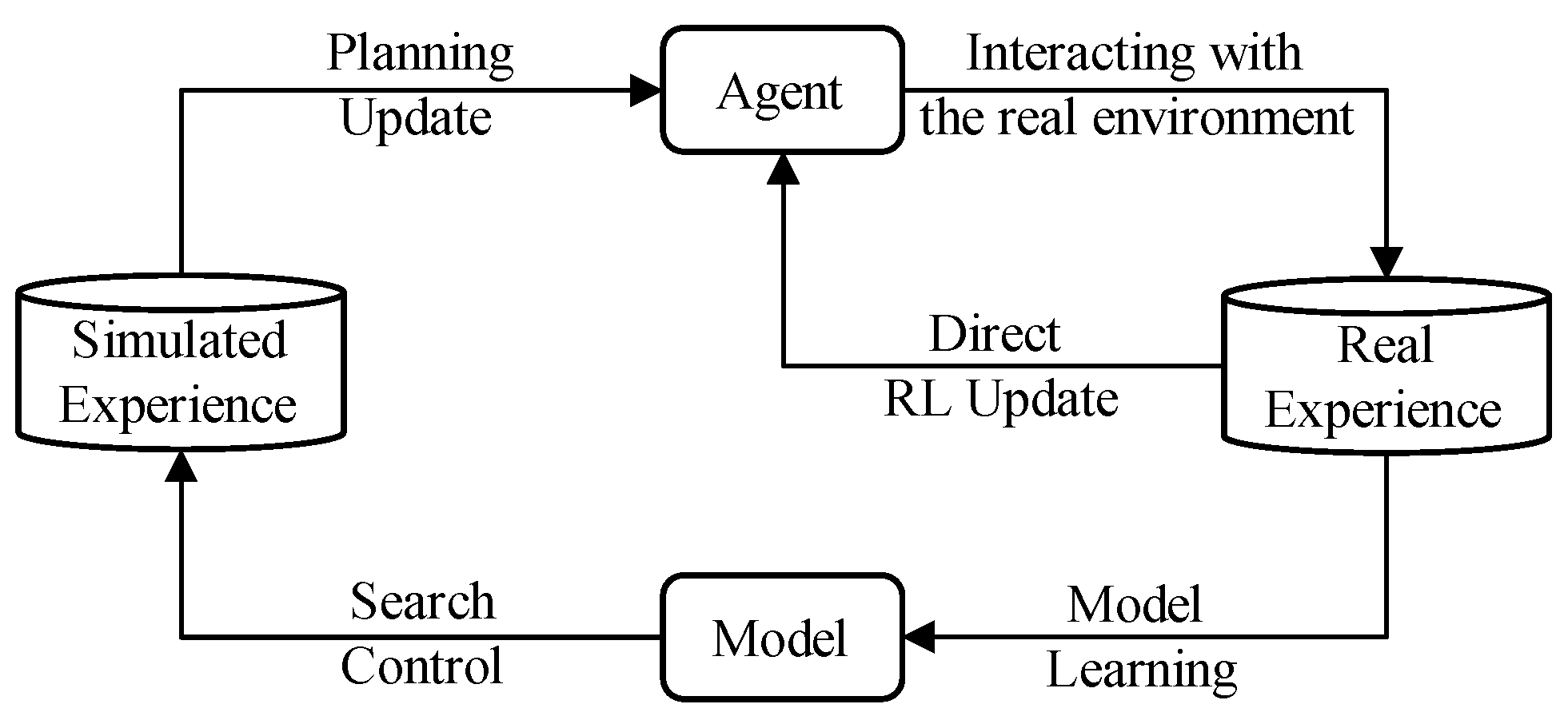
Definition 7. 

(Q-value updating)   A Q-value $Q(s,a)$ will be assigned when the AGV is located at state s and an action a is taken. The Q-function or the Q-value is updated using

$$Q(s,a)\leftarrow Q(s,a)+\alpha [r^{\prime }+\gamma \underset{a}{max}Q(s^{\prime },a^{\prime })-Q(s,a)]$$

(6)

where $Q(s,a)$ is the Q-value when the action a is executed at state a, ${max}_{a}Q(s^{\prime },a^{\prime })$ is the highest Q-value among all actions at next state $s^{\prime }$, α is the learning rate, and γ is the discount factor.

The Dyna-Q algorithm is a model-based RL method, which is the integration of planning and direct RL method. Planning is a process of optimizing strategies by using randomly generated simulation experiences through the learned environment model, while the direct RL method is to improve the value function and policy function by using the real experience generated by interaction with the environment, as shown in Figure 2. The Dyna agent interacts with the real environment to obtain empirical data and improves the algorithm policy by iterating through Equation (6); at the same time, an environment model is learned using real experiences, and the simulation data generated by the model are then used to update the action-value function using Q-Learning update method.

In the actual path planning task, real experiences obtained by interacting with the real environment are usually expensive and time-consuming, while using the learned environment model to generate simulation experiences is fast and convenient, thus reducing the training time of the algorithm.

When the Dyna-Q algorithm is applied to path planning in large-scale dynamic environments, there are also the following problems:

• In the path planning problem, the traditional reward function will update the reward only when reaching the destination or encountering obstacles. Especially in the face of large and complex environments, there are a large number of negative or invalid search spaces. Therefore, in large and complex environments, the traditional reward function has the problem of sparse rewards—that is, AGV is difficult to obtain positive rewards in the process of exploration, resulting in slow learning or even inability to learn.
• In the early stages of Dyna-Q, each step of the policy is exploratory. In addition, when Dyna architecture uses environment model planning, it randomly selects the state and action to update, which has certain blindness. Therefore, the application of Dyna-Q algorithm to path planning in a large-scale dynamic environment has the problems of low learning efficiency and long training time.

3. Improved Dyna-Q

In order to solve the problem of sparse reward, slow convergence, and long training time of Dyna-Q algorithm in large-scale dynamic environments, this paper proposes an Improved Dyna-Q algorithm. In this section, we first describe the basic concepts of heuristic graph, and then introduce the details of the method in this paper.

3.1. Heuristic Graph

In this study, AGV only has a local field of view—that is, it can only perceive the information of the current grid position. In the early stage of exploration, each step of RL strategy is exploratory. Especially in large and complex maps, it is difficult to reach the target location. Therefore, path planning in large and complex maps needs to rely on other information to enable the AGV to reach the target position quickly. Previously, researchers proposed distance metrics [25]. The quantitative value of distance measurement is evaluated based on the distance from the current position to the next state and target position. Distance measurement provides distance information about the current position to the target position. However, it does not provide information on environmental barriers. Therefore, when obstacles are complex, the disadvantage of using distance measurement is that the AGV may fall into a dead end [25].

In this study, a novel heuristic graph is first proposed, which contains the standardized shortest path distance information from each location in the whole map to its target location. It allows AGV to obtain a heuristic distance to the target. The purpose of proposing a heuristic information map is to provide sufficient information for AGV, guide AGV to quickly explore its target position as global guidance information, and avoid falling into the map area that leads to a dead end.

Definition 8. 

(Heuristic Graph $\mathcal{H}$)   A graph structure $\mathcal{H}(S,A)$ of size $W\times H$, with the same size of the graph as the environment map. The heuristic value of each position $s=(x,y),1\le x\le W,1\le y\le H$ in the heuristic graph is defined by Equation (7). The heuristic value for selecting action a in the current state s is given by Equation (8).

$$\mathcal{V}\left(s\right)=\left\{\begin{array}{c}0,s=Goal\hfill \\ 1,s\in V_s\hfill \\ \frac{shortestpathlength\left(s\right)}{(W+H)},s\in V_f\hfill \end{array}\right.$$

(7)

$$\mathcal{H}(s,a)=\mathcal{V}\left(s^{\prime }\right)$$

(8)

where $s^{\prime }$ is the position of the neighbor node after the selection of action a at position s.

$\mathcal{H}(s,a)$ represents the heuristic distance information of selection action a in the current state s—that is, the standardized path distance information from the adjacent node to the target node. The shortest path distance of each location in the map is calculated by performing Breadth First Search (BFS) in the entire static map from the target location. Heuristic graph implies static obstacle information. As shown below, the pseudo code for computing the heuristic graph is given in Algorithm 1.

Algorithm 1 get heuristic graph $\mathcal{H}$

Input: goal, Map[Height, Width]

Output:  $\mathcal{H}$

1: Initialization:Visited $\leftarrow \varnothing$, q ← Queue()

2: Goal.len ← 0

3: q.push(Goal)

4: Visited.add(Goal)

5: while not q.empty() do

6:    current = q.pop()

7:    for next in get_neighbors(current) do

8:        if next ∉ Visited then

9:         next.len ← current.len + len(current, next)

10:         q.push(next)

11:         Visited.add(next)

12:      end if

13:    end for

14: end while

15: for each s in Map do

16:    if Map[s] is Obstacle then

17:      $\mathcal{V}\left[s\right]$ = 1

18:    else

19:      $\mathcal{V}\left[s\right]$ = Visited[s].len/(Width+Height)

20:    end if

21: end for

The heuristic graph can be calculated in advance of the algorithm training policy; the heuristic graph is only calculated once and remains unchanged. During execution, the heuristic value can be obtained by retrieving the current position of AGV from the heuristic graph. Therefore, the impact of computing the heuristic graph on execution time can be ignored.

Definition 9. 

(Best heuristic action set $A_{\mathcal{H}}$)   The best heuristic action set is defined as the set of actions with the minimum heuristic value at the current state.

$$A_{\mathcal{H}}\left(s\right)=\arg \underset{a\in A}{min}\left(\mathcal{H}(s,a)\right)$$

(9)

The best heuristic action set indicates that the action in the set is executed at the current position, and the next position is closer to the target position—that is, those actions that make the next position closer to the target position.

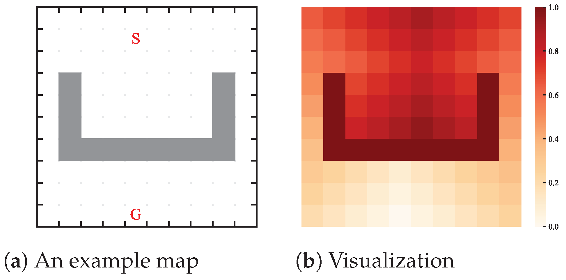
Figure 3 is the visualization of the heuristic map of a map instance. Figure 3a shows a map size of $10\times 10$, where ‘S’ represents the starting position of the AGV, ‘G’ represents the target position of the AGV, and gray squares represent static obstacles. Figure 3b shows the visualization of the heuristic graph of the map example on the left. The color squares from dark to light represent the size of the heuristic value. The darker the color of the current point, the greater the value of the heuristic graph of the current position—that is, the farther from the target position.

3.2. Improved Dynamic Reward Function

The reward function is used to determine the value of action. AGV interacts with the environment according to the reward function, and continuously optimizes the action policy through the reward value. The reward function must be designed to correspond to the target to be optimized. Therefore, the design of the reward function is crucial to the efficiency of the optimized problem. In most previous researches on reinforcement learning path planning, the reward values are usually a static value, which are obtained only when it reaches the target position or encounters obstacles. This reward design can easily reach the target position in a small map environment, and then converge to a shorter path. However, there is a sparse reward problem in long-distance navigation. According to the characteristics of the path planning problem, some scholars proposed a reward function related to the Euclidean or Manhattan distance. Compared with the traditional reward function, this method has a guiding effect on the exploration of mobile robots, and the convergence speed has been improved to a certain extent. However, this reward function does not take into account the information of obstacles, which easily leads to falling into the local optimal solution.

In this study, a novel dynamic reward function based on heuristic graph is proposed to provide AGV with intensive reward values. The dynamic reward function based on heuristic graph encourages AGV to explore all potential solutions, and AGV will encourage it to move closer to the target location at any location. Heuristic graph contains static obstacle information, which can effectively guide AGV to avoid concave obstacle areas, thus speeding up the convergence of the algorithm.

Definition 10. 

(Dynamic reward function $r_{\mathcal{H}}(s,a)$)    The dynamic function $r_{\mathcal{H}}(s,a)$ guides the AGV towards the goal in the direction of the reduced value in the heuristic graph, while avoiding collisions with dynamic and static obstacles. In detail, the dynamic reward function based on heuristic graph is defined as follows:

$$r_{\mathcal{H}}(s,a)=\left\{\begin{array}{c}{r}_1,s^{\prime }\in V_f\cap a\notin A_{\mathcal{H}}\left(s\right)\hfill \\ r_1+r_2,s^{\prime }\in V_o\cup V_d\hfill \\ r_1+r_3,a\in A_{\mathcal{H}}\left(s\right)\hfill \\ r_4,s^{\prime }\in Goal\hfill \end{array}\right.$$

(10)

where $s^{\prime }$ is the next position at which the AGV takes action a at time t, and $r_{\mathcal{H}}(s,a)$ denotes the immediate reward value of the action a taken by the AGV at time t.

More specifically, at each time, the dynamic reward function provides the following: (1) a small negative reward $r_1<0$ when the AGV reaches a free grid that is not a minimum heuristic value; (2) a large negative reward $r_1+r_2$ when the AGV conflicts with a static or a dynamic obstacle, where $r_2<r_1<0$; (3) a positive reward $r_3$ when the action performed by the AGV is the best heuristic action, where $r_3=\left|r_1\right|$; (4) a large positive reward $r_4$ when the AGV reaches the goal position.

Combined with the heuristic graph, the dynamic reward function mechanism provides intensive feedback signals for AGV. By this way, AGV is not required to strictly follow a global path but encouraged to explore all potential solutions to avoid falling into the local optimal solution; in the process of guiding AGV to the target position, avoid collision with dynamic obstacles at the same time, and finally converge to a collision-free and conflict-free optimal policy.

3.3. Improved Heuristic Planning

In order to solve the problem of high complexity, heuristic search increases knowledge in specific fields to improve search efficiency. Heuristic search uses the current information related to the problem as heuristic information to guide the search. Heuristic strategies can guide the search to select branches that are more likely to produce successful results than other methods, reduce the search scope, and reduce the complexity of the problem [28].

The model-based RL algorithm is divided into two parts: direct learning and planning. In the planning process, RL algorithm randomly generates simulation experiences from the model learned from practical experience, and then indirectly improves the value functions and strategies. In the path planning problem, there is a certain blindness in the process of randomly generating simulation experience. Inspired by the heuristic search algorithm, the previous work [30] believed that using heuristic planning to generate simulation experience in the planning process, and updating which states are closer to the target position is conducive to improving the learning efficiency of the algorithm, thus speeding up the convergence of the algorithm.

This paper uses heuristic graph $\mathcal{H}(S,A)$ as the heuristic function. During each planning, select the heuristic action with the minimum heuristic function value $\mathcal{H}(S,A)$ in the current state. When there are multiple minimum heuristic actions in the current state, randomly select one of them.

$$a_{\mathcal{H}}\left(s\right)=arg\underset{a}{min}\left(\mathcal{H}(s,a)\right)$$

(11)

Through the combination of heuristic graph and heuristic planning, update the most promising Q-values, further accelerate the learning efficiency of the algorithm, and reduce the training time of the Dyna-Q algorithm.

3.4. Improved Dyna-Q for Path Planning

In this paper, an Improved Dyna-Q algorithm for AGV path planning in dynamic environments is proposed. The basic idea is as follows: A global path guidance mechanism called heuristic graph is introduced, which combines heuristic graph and dynamic reward function to provide intensive rewards, guide AGV to move to the target position, and solve the sparse reward problem of long-distance path planning. Then, in the planning process of Dyna architecture, the heuristic graph information is used for heuristic search to improve the learning efficiency of the algorithm and reduce the training time of the algorithm.

Algorithm 2 gives a complete Improved Dyna-Q algorithm flow. Among them, $Model(s,a)$ is the learning environment model, which is used to predict the reward of the next state and state–action pair $(s,a)$, and n is a super parameter, which represents the steps of simulation planning. After AGV interacts with the environment and executes Q-Learning once, Dyna-Q will execute n times of planning. When n is 0, Dyna-Q becomes a classical Q-Learning algorithm.

Algorithm 2 Improved Dyna-Q algorithm

1: Initialize Q(s,a)=0, Model(s,a)=0

2: get heuristic graph $\mathcal{H}$

3: repeat

4:    $s\leftarrow$ initial state

5:    repeat

6:      $a\leftarrow$$ϵ$-greedy(s,Q)

7:      execute a; observe $s^{\prime }$ and $r_{\mathcal{H}}(s,a)$

8:      $Q(s,a)\leftarrow Q(s,a)+\alpha [r_{\mathcal{H}}(s,a)+\gamma {max}_{a^{\prime }}Q(s^{\prime },a^{\prime })-Q(s,a)]$

9:      Model(s,a) $\leftarrow s^{\prime },r_{\mathcal{H}}(s,a)$

10:      for $i=1:n$ do

11:         $\tilde{a}\leftarrow a_{\mathcal{H}}\left(s\right)$

12:         if s, $\tilde{a}$∉ Model($s,\tilde{a}$) then

13:           s ← random previously observed state;

14:           $\tilde{a}\leftarrow$ random action previously taken in state s;

15:         end if

16:         ${\tilde{s}}^{\prime },r\leftarrow$ Model(s,a);

17:         $Q(s,\tilde{a})\leftarrow Q(s,\tilde{a})+\alpha [r+\gamma {max}_{a^{\prime }}Q({\tilde{s}}^{\prime },a^{\prime })-Q(s,\tilde{a})]$

18:         $s\leftarrow {\tilde{s}}^{\prime }$

19:      end for

20:      $s\leftarrow s^{\prime }$

21:    until s is terminal

22: until the total number of episodes N is reached

4. Simulations and Results

In this section, the Improved Dyna-Q algorithm is compared with Dyna-Q and Q-Learning algorithm in a static environment by designing simulation experiments. Then, the proposed algorithm is evaluated and verified on the maps with different numbers of dynamic obstacles to show its advantages.

4.1. Environment and Parameter Configuration

All algorithms were implemented using Python 3.8. All simulation experiments were performed on Ubuntu 20.04 with NVIDIA RTX 1050 GPU and 16 GB RAM. The proposed algorithm is verified in a random obstacle map. The environment map is a 2-D grid world of size $50\times 50$ cells, the static obstacles are randomly generated according to an approximately normal distribution, and the random static obstacle ratio is $10\%$.

The algorithms used in this comparative experiment are Q-Learning, the original Dyna-Q, the Dyna-Q with only the improved dynamic reward function proposed in this paper (Dyna-Q with dynamic reward), and Dyna-Q with the two improvements proposed in this paper (Improved Dyna-Q). The parameters of the four algorithms are compared using the same values. The specific parameter configurations of the four algorithms are shown in

Table 1. Simulation parameters of configurations.

Parameter	Symbol	Value
Discount factor	$\gamma$	0.95
Learning rate	$\alpha$	0.2
Greedy factor	$ϵ$	0.1
Planning steps	n	10
Episode number	N	1000

.

4.2. Simulation Results

4.2.1. Static Environment

First, in the static map environment, this paper compares the path length of the Dyna-Q algorithm using the traditional reward function and the dynamic reward function improved in this paper with the number of iterations. The traditional reward function used in this paper is Equation (12), and the dynamic reward function is Equation (13).

$$r(s,a)=\left\{\begin{array}{c}10,s^{\prime }\in Goal\hfill \\ -0.5,s^{\prime }\in V_o\cup V_d\hfill \\ 0,otherwise\hfill \end{array}\right.$$

(12)

$$r_{\mathcal{H}}(s,a)=\left\{\begin{array}{c}-0.1,s^{\prime }\in V_f\cap a\notin A_{\mathcal{H}}\left(s\right)\hfill \\ -0.1+(-0.5),s^{\prime }\in V_o\cup V_d\hfill \\ -0.1+(+0.1),a\in A_{\mathcal{H}}\left(s\right)\hfill \\ 10,s^{\prime }\in Goal\hfill \end{array}\right.$$

(13)

Train 1000 times in a static environment, where the maximum number of AGV exploration steps in each episode is set to 2000. As shown in Figure 4, it can be seen that in the first 200 times of episodes using the traditional reward function, the path length is 2000 steps, which indicates that there is a sparse reward problem in complex environments and AGV cannot effectively update the policy. Only after full exploration can AGV reach the target position, which makes the running time of the algorithm longer. The dynamic reward function mechanism proposed in this study can effectively guide AGV to explore the target location. Intuitively, the convergence speed of the dynamic reward function proposed in this paper is much faster than that of the traditional reward function.

Secondly, the simulation experiments of four algorithms—Q-Learning, Dyna-Q, Dyna-Q with dynamic reward, and Improved Dyna-Q—are carried out in the static environment map. Figure 5 shows the path planning trajectory obtained after 1000 training sets using the four algorithms. It can be seen from the path trajectory diagram that Q-Learning did not find the shortest path, while the paths of the other three Dyna-Q algorithms are obviously better than that of Q-Learning algorithm. Intuitively, the Improved Dyna-Q algorithm proposed in this paper is superior to other algorithms in distance and direction. Figure 6 shows the learning curve of the four algorithms in the static environment map. The Q-Learning algorithm shows a very slow convergence curve; in fact, it never found the optimal policy. The convergence speed of the Dyna-Q algorithm is greatly improved compared with that of Q-Learning, mainly because Dyna-Q learned an environment model and improved the auxiliary policy. The Improved Dyna-Q algorithm proposed in this paper has the fastest convergence speed. Compared with the Dyna-Q algorithm, the improved dynamic reward function method and the Improved Dyna-Q algorithm greatly improved the convergence speed.

Although the convergence curve trend of the Improved Dyna-Q algorithm using the dynamic reward function proposed in this paper is the same as that of the Improved Dyna-Q algorithm using the two improvement points proposed in this paper, the running time of the algorithm proposed in this paper is the shortest, as shown in

Table 2. Performance comparison of four algorithms in static obstacle environments.

		Q-Learning	Dyna-Q	Dyna-Q with Dynamic Reward	Improved Dyna-Q
path length (unit)	min	124	82	82	82
	max	211	89	91	88
	mean	171.03	86	86.59	82.37
train time (s)	min	34.86	275.28	59.29	12.3
	max	36.53	321.31	70.68	13.96
	mean	35.64	298.8	64.88	12.94

. Table 2 shows the performance comparison of four algorithms trained 1000 times in the static map. Each algorithm was repeated 30 times. In the path length index, the minimum path length of the Dyna-Q, Dyna-Q with dynamic reward, and Improved Dyna-Q algorithms is 82, indicating that the three algorithms have found the optimal strategy. Because of its slow convergence speed, the Q-Learning algorithm failed to find the optimal strategy in 1000 iterations. The average calculation time of using the improved dynamic reward function proposed in this paper is reduced by $81.83\%$, because the dynamic reward function not only solves the sparse reward problem but also guides the AGV to search the target location, significantly reducing the useless search space. Furthermore, compared with Dyna-Q with dynamic reward, the average running time of the Improved Dyna-Q algorithm using both improved heuristic planning and improved dynamic reward function has increased by $80.01\%$, which shows that the improved heuristic planning can help speed up the running time of the algorithm. On the whole, the average path length of the algorithm proposed in this study is the shortest, and the average computing time is $95.67\%$ less than that of Dyna-Q algorithm.

4.2.2. Dynamic Environment

In this paper, 10, 20, and 30 dynamic obstacles are randomly added to the random static obstacle map. The three maps with different numbers of dynamic obstacles are shown in Figure 7. Each dynamic obstacle moves back and forth from its starting point to the target point, and the shortest path of the dynamic obstacle is generated by A* algorithm.

Table 3. Performance comparison of four algorithms in environments with different numbers of dynamic obstacles.

			Q-Learning	Dyna-Q	Dyna-Q with Dynamic Reward	Improved Dyna-Q
10 dynamic obstacles	path length (unit)	min	125	83	82	82
		max	167	85	86	86
		mean	146.3	83.7	84.1	83.9
	train time(s)	min	42.86	302.38	65.54	13.29
		max	44.08	325.78	71.88	14.64
		mean	43.4	309.21	68.09	14.18
20 dynamic obstacles	path length (unit)	min	127	83	82	82
		max	172	90	90	89
		mean	155.6	84.4	85.4	84.9
	train time(s)	min	43.12	321.41	66.12	14.04
		max	44.76	368.21	82.78	16
		mean	43.95	341.46	77.44	15.06
30 dynamic obstacles	path length (unit)	min	130	82	82	82
		max	173	84	84	89
		mean	146.8	82.6	82.9	85.4
	train time(s)	min	47.68	316.51	65.54	14.61
		max	49.9	340.07	74.68	17.09
		mean	48.59	328.01	70.57	15.39

shows the performance comparison of four algorithms trained 1000 times in three kinds of dynamic obstacle environments, in which each algorithm is repeated 30 times. Compared with the static obstacle environment, the average path length of all algorithms increased, mainly because the algorithm needs to avoid dynamic obstacles. Among the three maps with different dynamic obstacle numbers, the Improved Dyna-Q algorithm has little difference with Dyna-Q in the average path length; however, in the training time index, the Improved Dyna-Q algorithm is obviously superior to the other three algorithms.

5. Conclusions

In recent years, reinforcement learning has been favored in path planning research. Dyna-Q is a reinforcement learning method widely used in AGV path planning. However, this method has the problems of low search efficiency and slow convergence speed. An Improved Dyna-Q algorithm is proposed to solve the path planning problem of AGV in dynamic environments. This research first proposes a global path guidance mechanism based on heuristic graph, which can effectively reduce the path search space and improve the convergence speed of the algorithm. Secondly, based on the heuristic graph, this paper proposes a new dynamic reward function and a heuristic action selection method to provide more intensive feedback signals and more efficient action selection for AGV path planning.

To demonstrate the advancement of the proposed algorithms, different simulation experiments are carried out in this paper. The numerical analysis results show that the proposed algorithm significantly speeds up the convergence speed and computation time of the algorithm compared with the classical Dyna-Q algorithm, and the Improved Dyna-Q algorithm can effectively solve the AGV path planning task in different dynamic obstacle count environments.