Article

Mapping Temperate Forest Phenology Using Tower, UAV, and Ground-Based Sensors

1
Department of Biology, Virginia Commonwealth University, Richmond, VA 23284, USA
2
NASA Goddard Space Flight Center, Greenbelt, MD 20771, USA
3
Department of Environmental Sciences, University of Virginia, Charlottesville, VA 22904, USA
*
Author to whom correspondence should be addressed.
Drones 2020, 4(3), 56; https://doi.org/10.3390/drones4030056
Submission received: 12 July 2020 / Revised: 4 September 2020 / Accepted: 6 September 2020 / Published: 10 September 2020

Abstract

:
Phenology is a distinct marker of the impacts of climate change on ecosystems. Accordingly, monitoring the spatiotemporal patterns of vegetation phenology is important to understand the changing Earth system. A wide range of sensors have been used to monitor vegetation phenology, including digital cameras with different viewing geometries mounted on various types of platforms. Sensor perspective, view-angle, and resolution can potentially impact estimates of phenology. We compared three different methods of remotely sensing vegetation phenology—an unoccupied aerial vehicle (UAV)-based, downward-facing RGB camera, a below-canopy, upward-facing hemispherical camera with blue (B), green (G), and near-infrared (NIR) bands, and a tower-based RGB PhenoCam, positioned at an oblique angle to the canopy—to estimate spring phenological transition towards canopy closure in a mixed-species temperate forest in central Virginia, USA. Our study had two objectives: (1) to compare the above- and below-canopy inference of canopy greenness (using green chromatic coordinate and normalized difference vegetation index) and canopy structural attributes (leaf area and gap fraction) by matching below-canopy hemispherical photos with high spatial resolution (0.03 m) UAV imagery, to find the appropriate spatial coverage and resolution for comparison; (2) to compare how UAV, ground-based, and tower-based imagery performed in estimating the timing of the spring phenological transition. We found that a spatial buffer of 20 m radius for UAV imagery is most closely comparable to below-canopy imagery in this system. Sensors and platforms agree within +/− 5 days of when canopy greenness stabilizes from the spring phenophase into the growing season. We show that pairing UAV imagery with tower-based observation platforms and plot-based observations for phenological studies (e.g., long-term monitoring, existing research networks, and permanent plots) has the potential to scale plot-based forest structural measures via UAV imagery, constrain uncertainty estimates around phenophases, and more robustly assess site heterogeneity.

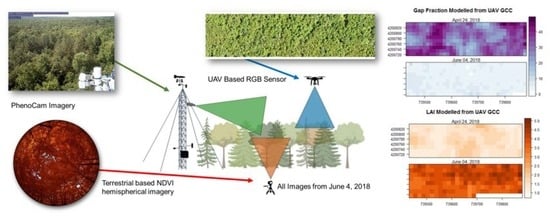
Graphical Abstract

1. Introduction

Spring phenology in temperate forests is a biological indicator of the near-term impacts of climate change [1]—regulating photosynthesis [2]; thus, driving primary productivity and carbon cycling. Warming trends have resulted in both an advancement in the onset of spring vegetation activity phenophase, or leaf-out, and an extension of the growing season across the globe [3,4]. It is necessary to quantify changes in the timing of phenophases that accompany anthropogenic climate change in order to constrain uncertainties in modeling the Earth system [5]. Near-surface optical remote sensing, specifically suborbital and ground-based methods, are well-suited for phenological observation [6], with the most commonly used sensors being RGB cameras—cameras that capture reflectance in the red, green, and blue channels. For phenological observation, RGB cameras can be used either above-canopy (from the air, unoccupied aerial vehicles (UAV)), below-canopy (tripod-based or ground-based, facing upwards into the canopy), or at oblique-view angles (often tower-based, looking across the top-of-the-canopy). Comparisons of optical sensors have shown they are robust [7,8,9,10,11], but cross-platform validation of how view angle or observation perspective of the canopy influences canopy-level phenological assessment is necessary to inform scaling. UAV based sensors offer substantial potential to upscale plot observations to the stand or landscape level at finer resolutions than spaceborne platforms (e.g., MODIS, Landsat), but this potential must be informed by in situ measurements to be fully realized as remote sensing methods are best when informed by ground-validation.
UAV-based sensors partially fill an extant gap in observational resolution and extent, while offering substantially higher temporal resolution than can realistically be garnered with spaceborne mapping. In phenological, as well as ecological research broadly, there are trade-offs in observational extent and resolution, in both space and time. This becomes an optimization problem where either resolution or extent must be prioritized. For example, spaceborne sensors that provide global coverage such as MODIS and AVIRIS that have relatively short return intervals provide relatively high temporal resolution on the order of 10 s of days, but do so by sacrificing spatial resolution. Conversely, small commercial satellites (e.g., CubeSats) can provide sub-meter spatial resolution with daily return intervals, but only over specific, highly limited spatial extents. UAV imagery can be collected over areas on the order of hectares in just a few hours; thus, providing an advantage in spatial extent over stationary RGB imagery [12,13]. There are trade-offs however, as UAVs do require licensed operators and their use may be restricted by local ordinances or laws which almost universally require UAVs to remain in “line-of-sight”. Further, UAVs may also be constrained by weather and battery life which can limit or prevent data collection. The nadir view-angle of UAV-based sensors (i.e., downward-facing) may introduce potential obfuscation and errors that are not associated with the oblique angle of tower-based sensors. These limitations have not hindered the adoption of UAV imagery for phenological study as the advantages outweigh the disadvantages [10,14], however, forested ecosystems have thus far been comparatively underrepresented [9,15,16,17,18]. Research on tree-level phenology in temperate [16] and tropical systems [18] illustrates the potential of UAV imagery as a means to account for site heterogeneity and more precisely quantify the spatial distribution of phenological timing. Multi-temporal UAV-based studies in forest systems can provide detailed insight into the spatial drivers of phenological phenomenon and must be evaluated in a range of ecosystems.
RGB cameras are powerful phenological tools because indices of plant greenness, such as the Green Chromatic Coordinate (GCC), a ratio of the green channel to all RGB channels, can be derived from standard RGB imagery [19]. GCC is well correlated with canopy development, leaf-out, and photosynthesis [20,21]. GCC is one index used widely by the PhenoCam network, a network of over 400 cameras across North America (as of 2020), each uploading images to a server every 30 min [22]. Data from these cameras are made publicly available free of charge, as are open-source software solutions to interpret and analyze PhenoCam data. Repeat RGB imagery, such as the PhenoCam network [22], has the advantage of consistency and high-temporality. The images collected can readily be compared to each other and end-users know the data are always the same areas of the canopy, from image to image. However, PhenoCam data provide snap shots of only one area of the canopy, which limits the assessment of site heterogeneity.
Below-canopy observation is often conducted with cameras outfitted with hemispherical lenses, mounted on tripods, facing upwards into the canopy [23]. This method has the advantage of isolating the canopy, which removes any interference from the ground or understory vegetation. Ground-based methods of capturing phenology are limited by user mobility, image quality, sun angle, and sky conditions. On clear sky days, early morning or late evening hours are preferable. Isolating the canopy allows for the estimation of additional forest structural metrics, such as leaf area index (LAI) and canopy gap fraction, which are not necessarily directly inferable from all other sensors surveyed here [24]. In addition to, or in replace of, standard RGB channels, cameras can include near-infrared (NIR) channels, which allow the calculation of the normalized difference vegetation index (NDVI), a common index in spaceborne remote sensing that relates the red and NIR channels in imagery to estimate plant greenness and vitality [25,26]. For near-surface remote sensing, the blue channel can be used in place of the red channel in calculating NDVI.
There are large differences in the spatial extents that can be efficiently measured using the sensors we surveyed. Below-canopy cameras capture only point-measurements of limited areas of the canopy—capturing on the order of tens to thousands of square meters of canopy area as compared to thousands or more in the case of tower-based PhenoCams, or rather continuous UAV imagery, which can cover on the order of hectares [9]. The additional canopy structural information provided by below-canopy imagery could scale from the plot- to stand-scale with coincident UAV imagery. Given the difference in spatial extent, resolution, and perspective, however, it is necessary to quantify the resolution at which UAV imagery is most comparable to hemispherical imagery.
The purpose of this study is to assess three methods of recording vegetation phenology: (1) a ground-based, below-canopy, upward-facing digital single-lens reflex (DSLR) camera commercially designed for vegetation studies with B, G, and NIR channels; (2) a UAV-based, downward-facing or nadir-view RGB camera; and (3) a tower-based, oblique-perspective, RGB camera specifically designed for phenological study as part of the PhenoCam network. Comparisons among these sensors are necessary in order to understand what elements of phenology are being represented from any specific perspective, as well as how combining these measurements may provide more representative measurements of vegetation phenology. To this end, we tested each of these approaches in a mixed, temperate forests across the spring phenophase transition to full canopy closure in 2018 to answer the following questions:
  • At what spatial extent are above-canopy (UAV-based imagery) remote sensing metrics most representative of below-canopy (ground-based, hemispherical photography) vegetation metrics?
  • Do above- and below-canopy measures provide similar phenological transition dates as continuous phenological observational data, including oblique-perspective PhenoCam data, and spaceborne, MODIS, and Landsat data?

2. Materials and Methods

2.1. Site Description

Our study site is an unmanaged, mixed-temperate secondary forest located at the Pace Estate (37.9229, −78.2739), a property in holding of the University of Virginia, near Palmyra, Virginia, approximately 20 miles east of Charlottesville. The forest has an average stem density of 1813 trees ha−1, and is populated by Acer rubrum, Quercus alba, Fagus grandifolia, Pinus virginiana, and Nyssa sylvatica of similar composition to other mesic, temperate mid-Atlantic secondary growth forests, and has no recorded history of management during the past century. Precipitation averages 1240 mm y−1 with a mean annual temperature of 13.9 °C [27,28].

2.2. Above-Canopy, UAV-Based Measurements

We used a Mavic Pro outfitted with the stock 12.3 MP RGB camera with a 35 mm equivalent lens with an ISO range of 100–1600 and <1.5% distortion focus (DJI, Shenzhen, China). (Figure 1). We used DroneDeploy (DroneDeploy; San Francisco, CA, USA) to plan the flight path around the tower with 88% of front and side overlap and a flight altitude of 100 m. The white balance of the drone’s onboard camera was set to a fixed color temperature of 6000K. After data collection, we used PhotoScan (Agisoft; St. Petersburg, Russia) to create orthomosaic images with spatial accuracy of 1–2 m and resolution of 0.03 m. These data were rasterized and clipped to a rectangular bounding box around the plots of approximately 5.5 ha (37.9225, −78.276 to 37.9325, −78.275) for further analysis. We then derived Green Chromatic Coordinate (GCC) values from the red, green, and blue channels of the UAV orthoimagery, with GCC calculated using the following equation [20]:
GCCUAV = DNG/(DNR + DNG + DNB)
where DN represents the digital number (0 to 255) for the red (DNR), green (DNG), and blue (DNB) channels. GCC is less sensitive to differences in canopy illumination or in differences among cameras [20]. Orthoimage reconstruction was not fully successful for the 7 May 2018 (DOY 127) orthoimage, resulting in the removal of approximately half of the cropped scene (including four camera plots).

2.3. Below-Canopy Measurements

We used a 24 Megapixel Sony 6000 DSLR Compact 2571 camera (Regent Instruments; Quebec, QC, Canada) with a 180° hemispherical lens with a maximum field-of-view of 90° to capture hemispherical canopy imagery (Figure 1). The camera has three bands—blue, green, and NIR. To calculate NDVI, blue is used as the absorption band and NIR is used as the reflectance band. This differs from space-based NDIV approaches where the red channel is the absorption band since the blue channel is more scattered due to atmospheric Rayleigh scattering. For ground-based and UAV-based vegetation applications, the blue channel allows for superior band discrimination.
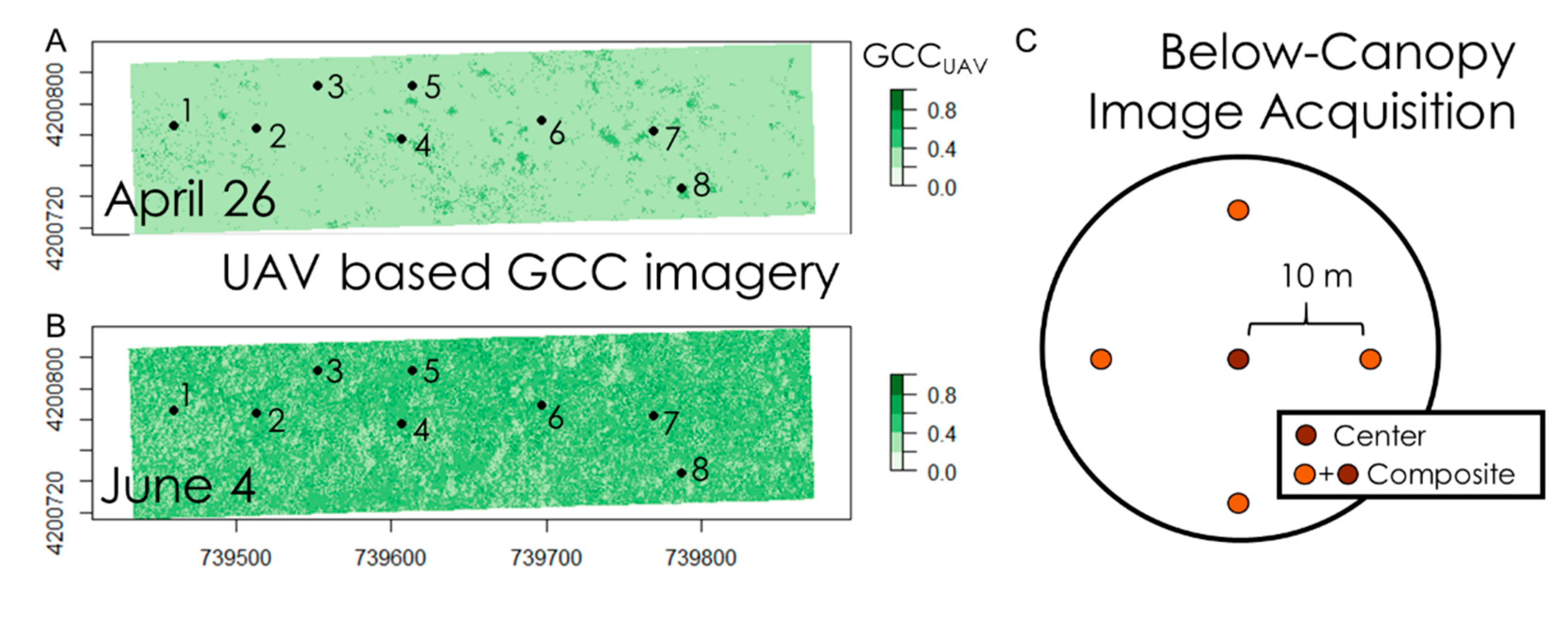
The camera was mounted on a self-leveling tripod, with the lens at 1 m from the ground, facing-upwards, looking into the canopy. At each plot location, five images were taken during the early morning hours (before 1000), approximately, weekly from late April until late May—at center, and 10 m off center at cardinal directions (Figure 2). For April 26 images, we used the “sunblocker,” a small, nylon disk supplied by the manufacturer attached to a flexible rod that is used to block the sun from the lens—the “sunblocker” is then masked out of the image later during analysis. For the first week of June, only images taken at plot center are available. We used image sets for analysis only during periods where there was coincident UAV-based imagery.
We calculated leaf area index (LAI), NDVI, and gap fraction for each image using WinSCANOPY (Regent Instruments; Quebec, QU, Canada) with a hemispherical image radius of 1925 px (total image size is 6000 × 4000 px) using a pixel color classification algorithm in WinSCANOPY that is more tolerant to variations in sky conditions, allowing the use of images with dark blue sky or partial-cloud coverage. Color-based classification palettes were established for each measurement period.

2.4. Tower-Based Measurements

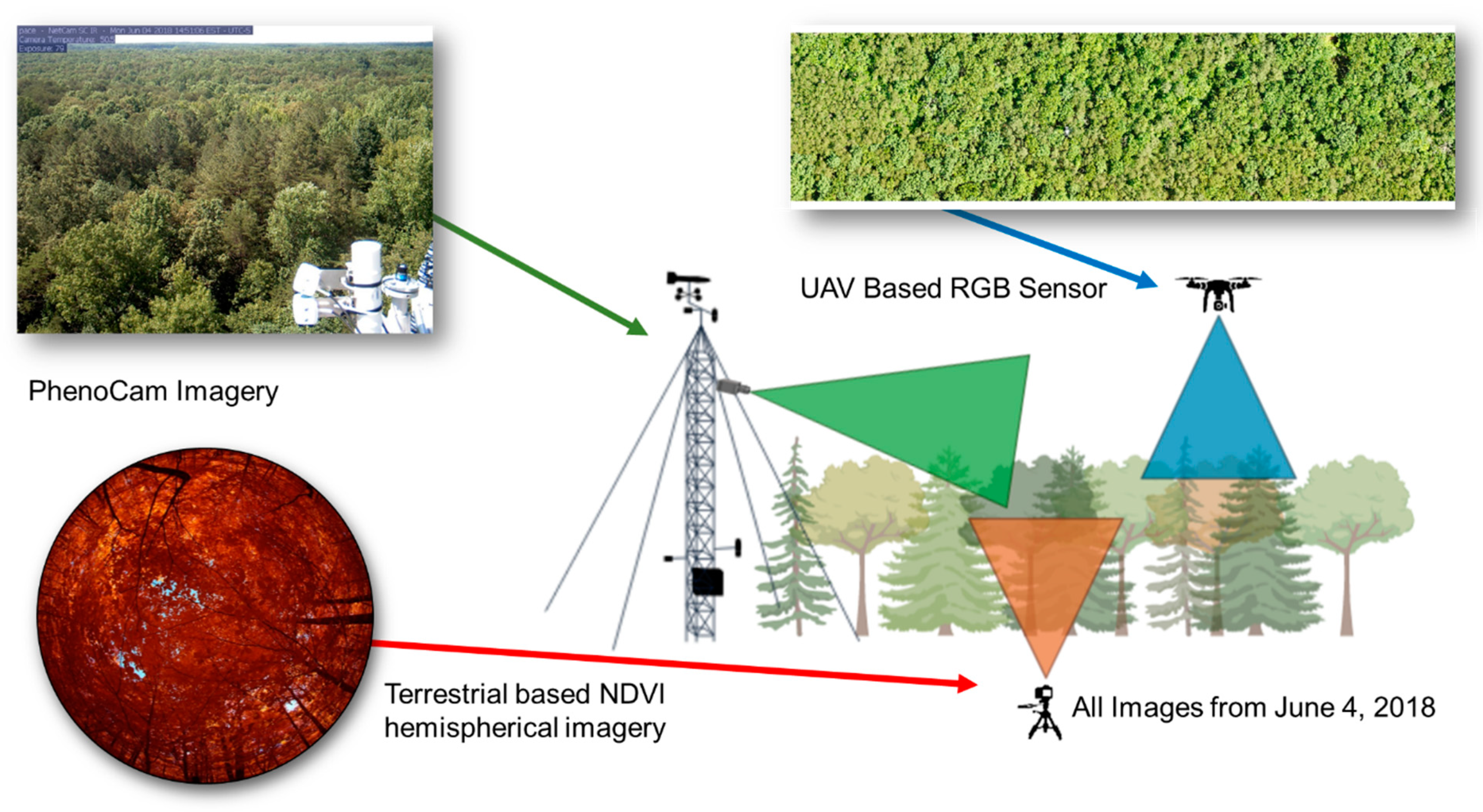
For the oblique-view of the forest canopy, we used the tower-based, RGB PhenoCam camera mounted to the Pace Estate eddy covariance tower (Figure 3). We accessed PhenoCam data from this camera acquired with the phenocamr package [29] in R 3.6.2 (R Core Team) for site “pace” where we downloaded and analyzed 3-day time interval data following the phenocamr documentation suggested package workflow: (1) data expansion; (2) outlier detection; (3) smoothing; (4) phenophase calculation. Full details on the process are available in the phenocamr vignette that is included in the package. This workflow provides “rising” phenophase dates informed by PhenoCam GCC values (GCCPC).

2.5. Satellite-Based NDVI

We incorporated two common satellite-based NDVI products into our analysis to provide a baseline to large-scale phenological studies: MODIS and Landsat 8 [30]. For each, we extracted NDVI from analysis-ready composite datasets available on Google Earth Engine, specifically the MOD13Q1 V6 Terra Vegetation Indices 16-Day Global 250 m product and the Landsat 8 Collection 1 Tier 1 8-Day NDVI Composite. We compiled all available scenes for both products as a time series of means and standard deviations of pixel values within the study extent. Statistics were computed for edge pixels with an area-based weighting of pixel values partially within the study extent.

2.6. Statistical Analysis

To address question one, we compared UAV data to below-canopy imagery using two different approaches. For the first, only images taken at plot center for each period were used—these data are noted as center in all text, tables, and figures. For the second approach, we used all available images per plot, per measurement period, averaged to make a plot level mean of NDVI, LAI, and gap fraction (Figure 2). These are denoted as composite in all text, tables and figures. Note, this does mean that there is no June imagery used in composite analyses. To test for the appropriate spatial extent with which to scale plot data with coincident UAV imagery, we averaged GCCUAV at increasing distances from plot center, starting at a 5 m buffer (i.e., distance from plot center) and increasing iteratively by 1 m, to a maximum of 50 m. The range of 5 to 50 m radius was chosen based on assumptions of how much canopy the hemispherical camera can see given its focal length. Standard forestry inventory plots rarely exceed 20 m in radius, thus making this range of comparison reasonable, even when considering that forest canopies associated with trees whose boles would be situated within a plot, will extend up to 5 m outside of the plot boundaries [20]. This was done for each of the 8 plots, for each of the 5 measurement periods, resulting in a total of 1147 clipped raster grid cells of mean GCCUAV. Note, that for 7 May 2018 (DOY 127), only 5 plots were used due to the orthoimage error (see Section 2.2 above). Linear regression was used to evaluate relationships among buffer size of GCCUAV with below-canopy measures of NDVI, LAI, and gap fraction with goodness-of-fit determined based on coefficient of determination (R2), directionality and internal calibration from the slope, and uncertainty quantified as residual mean standard error (RMSE). Moreover, 95% Confidence intervals were determined using bootstrapping analysis via the boot package in R [31,32].
We used the buffer size analysis on center and composite imagery to inform upscaling of both LAI and gap fraction from the plot to the entire UAV scene. For LAI, a 15 m buffer size was chosen to scale GCCUAV data to LAI using a linear model:
LAI = mGCCUAVb
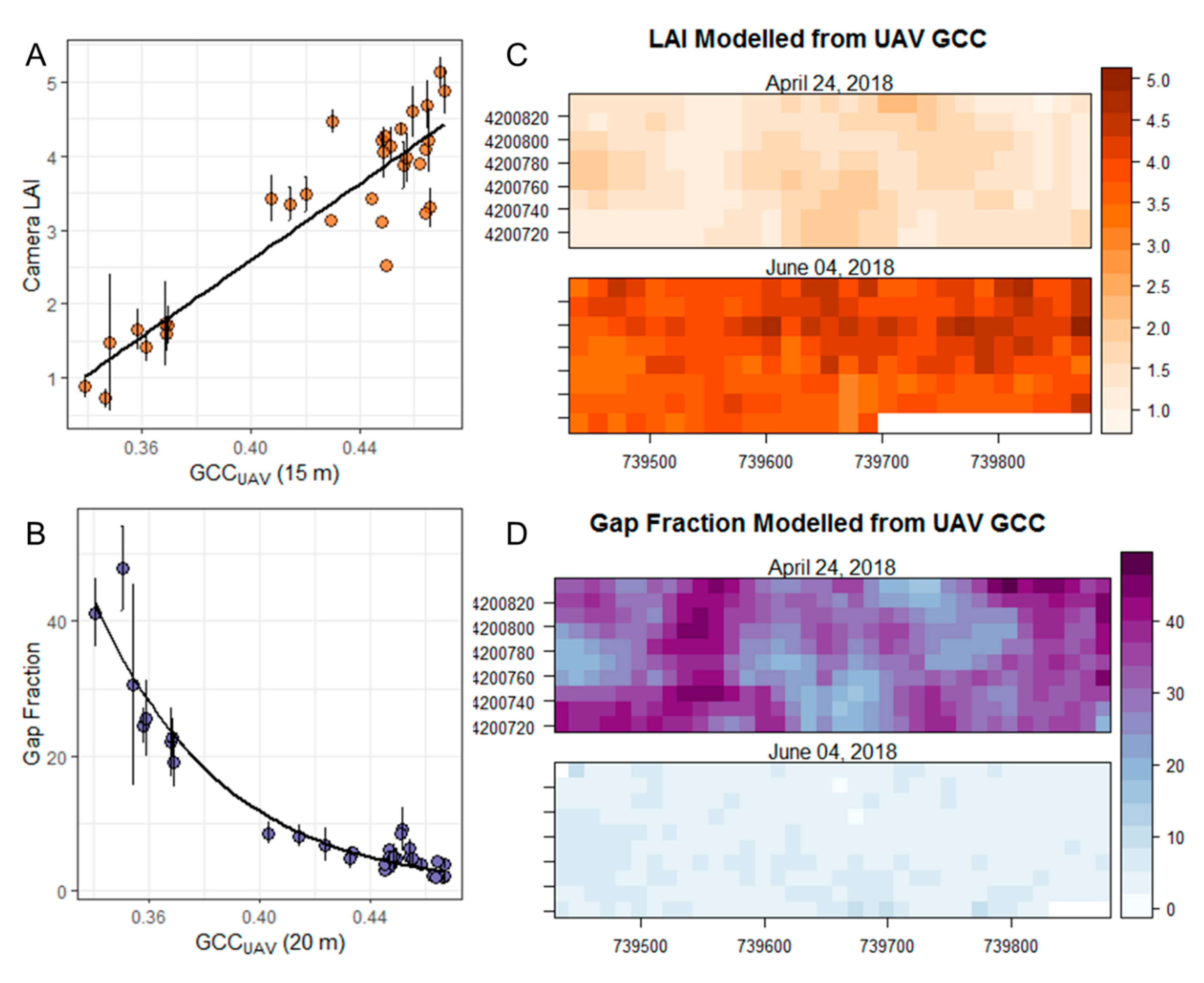
We chose a 20 m buffer size to scale GCCUAV to gap fraction. While we have included the iterative linear regressions statistics for gap fraction (Figure 4g), for upscaling purposes, we chose a non-linear model based on our analysis that better fit the data using non-linear least-squares via the nls function in R 3.6.2.:
G a p   F r a c t i o n = a e ( b   G C C U A V )
Rasters were resampled using bilinear sampling with the rgdal [33] and raster [34] packages in R 3.6.2 [35] to the appropriate resolution—15 m for LAI and 20 m for gap fraction. This was not done for NDVI, as GCCUAV and NDVI are already similar and the intent is to test the certainty with which LAI and gap fraction may be inferred from UAV imagery.
To address question two, we used breakpoint analysis with the segmented package [36] in R 3.6.2 to determine how each method estimates the phenological transition, specifically canopy closure. Breakpoint analysis, specifically segmented or piecewise regression, identifies thresholds that indicate critical changes in the directionality or slope of a dataset. On phenological data this method will indicate when the canopy is no longer increasing in “greenness,” indicating stability that we interpret as canopy closure. To evaluate how representative plot averages of GCCUAV were of the entire forest, means of whole scenes were compared against plot level means using root mean square error. For analysis scripts, code, and data, see Supplementary Materials.

3. Results

3.1. Above- and Below-Canopy Comparisons

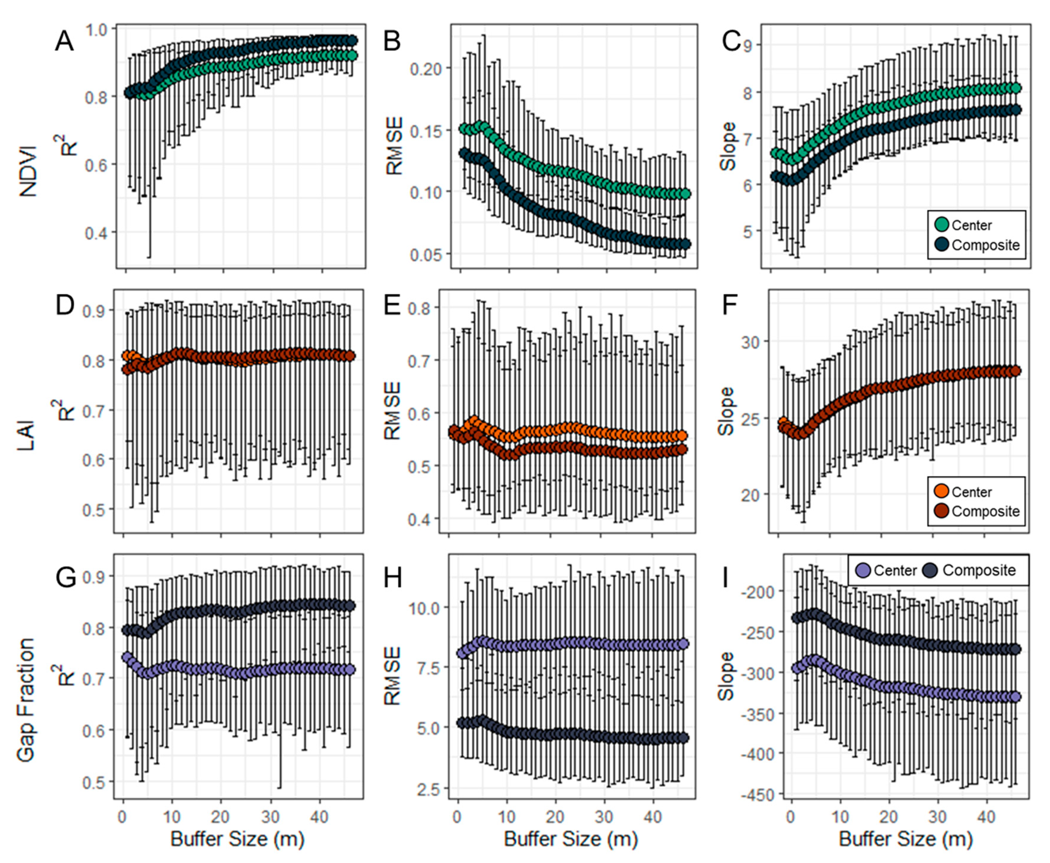
NDVI explained a large portion of variance in GCCUAV for both center and composite below-canopy imagery based on linear regressions with R2 values of 0.88 at 20 m for center imagery and 0.92 at 20 m for composite imagery (Figure 4a). R2 for both center and composite imagery continued to rise with increasing buffer size, before stabilizing around 35 m. RMSE values dropped consistently with buffer size as well, with RMSE at 20 m buffer size of 0.12 for center imagery and 0.08 for composite imagery (Figure 4b). Regression slopes were consistently positive with increasing buffer size (Figure 4c). While composite imagery showed increased explanatory power, confidence intervals show this effect is small to insignificant, though confidence intervals do become more constrained after ~ 15 to 20 m buffer sizes.
There were only small differences in LAI between center and composite imagery, though confidence intervals were consistently large, showing no constraint as buffer size increased. At 20 m, R2 was 0.80 for both center and composite imagery, while RMSE was 0.56 for center imagery and 0.53 for composite imagery. Slopes for both were nearly identical and increased steadily with buffer size. Peak agreement, based on R2, between above- and below-canopy imagery was in the 14 to 16 m buffer sizes, showing that increasing area of above-canopy GCCUAV averaging did not add additional information as it did in the case of NDVI. For scaling purposes, linear regression fit at 15 m buffer size was chosen for the scaling analysis, with coefficients of a = 25.77 and b = −7.71 (Equation (3)). These data provide us with confidence that, 15 m and 20 m, are appropriate resolutions to scale LAI and gap fraction, respectively. A non-linear function was chosen over a linear function to scale gap fraction, with coefficients of a = 65,354.32 and b = −21.55 for Equation (4). The non-linear function was chosen as the residual standard error was lower (3.20 vs. 4.87 for NLS and linear, respectively).

3.2. Estimating Canopy Closure

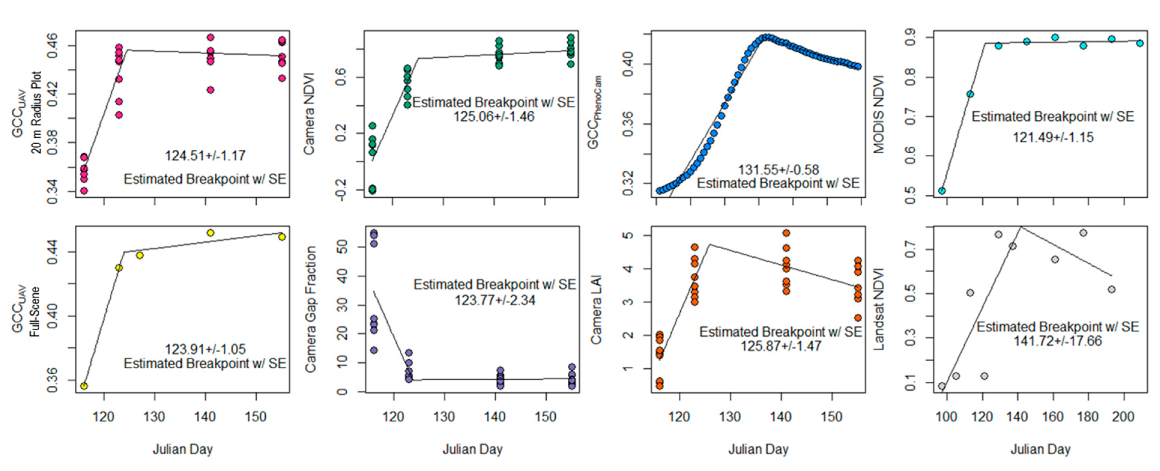
Transition from spring phenophase to canopy closure based on breakpoint analysis agreed among local-scale sensors, but differed substantially from Landsat 8 and MODIS. GCCUAV (full scene), GCCUAV (20 m buffer), NDVI, gap fraction, and LAI all show canopy closure to occur around DOY 124, with standard error that overlap among the variables, indicating no operational difference. GCCPhenoCam shows canopy closure to occur on DOY 131 however, nearly a week after above- and below-canopy sensors (Table 1; Appendix A1). MODIS shows the earliest indicated period of canopy closure at DOY 121, while Landsat shows both the latest day at DOY 141, as well as the greatest variance of over 17 days plus or minus, compared to 2 days or less for the majority of other sensors (Table 1.).

4. Discussion

Here, by comparing three similar sensors with different canopy perspectives—UAV-based RGB imagery, tower-based PhenoCam, and ground-based, below-canopy NDVI hemispherical imagery—we show strong, positive correlations among the rate and magnitude of canopy greening consistent across all sensors, regardless of the perspective which they view the forest canopy. Spatial resolution affects canopy structural variables derived from below-canopy hemispherical imagery and UAV imagery (e.g., LAI and gap fraction), but we demonstrate that these structural attributes can still be accurately inferred in temperate, broadleaf systems. Our analyses show that all three sensor platforms considered here effectively approximate phenological indicators, with above- and below-canopy methods estimating canopy closure earlier than the oblique-angle tower-based PhenoCams, but later than MODIS derived NDVI.

4.1. Scaling Above- and Below-Canopy Imagery

We found there are optimal, but differing plot radii over which GCCUAV is averaged that best approximates below-canopy measured NDVI and structural attributes, LAI, and gap fraction. As the averaging area for GCCUAV increases, the relationship between below-canopy measured NDVI and GCCUAV strengthens as evidenced by increasing values of R2 that are accompanied by narrowing confidence intervals (Figure 4). The statistical relationship between NDVI and GCCUAV stabilizes around 35 m in buffer size where R2 becomes asymptotic. We also observe a marked reduction in the size of the confidence intervals around 20 m. Composite imagery consistently outperformed center-only imagery, though the effect appears to be small. For LAI, however, the 14 to 16 m buffer size range resolved the most variance, followed by a decrease in R2 values at greater buffer sizes. The small difference between center and composite imagery indicates no apparent advantage to composite imagery over center-only imagery.
The strong agreement between GCCUAV and both LAI and gap fraction is sufficient to scale these findings via the UAV-based metric. Similar to Keenen et al. [37], we observed non-linear relationships between GCCUAV and gap fraction (S1) which indicates saturation of greenness at high levels of leaf area and low levels of gap fraction. Comparing our late April to early June measurements, we see consistent greening leading to consistent decreases in gap fraction. These relationships are strong for this forest type, but it is unknown how a more heterogeneous forest (e.g., patchy disturbance, more species diverse) would compare. Given our interpretation of the data, we suggest that LAI would be more variable than gap fraction, or even NDVI/GCC, in a more heterogeneous forest than our even-aged, predominately broadleaf temperate forest.
We also show that each sensor approximates dormant to growing season transitions to full-canopy closure within +/− 2 days, which is in line with the MODIS estimate, though MODIS data estimates a slightly earlier transition. However, PhenoCam estimates are 5 days later, a finding concurrent with other work [37]. Landsat 8 provides the latest canopy closure date nearly 15 days later than other sensors, likely due to longer return intervals and higher likelihood of less quality data due to cloud cover. While it is out of the scope of this work, the 20 m radius buffer we show is suitable for comparison between above- and below-canopy measures of phenology (Figure 5), and potentially structural attributes, and within the sensor capabilities of some spaceborne remote sensing platforms such as, but not limited to, Harmonized Landsat Sentinal-2 (10–20 m) or Planet Labs (3–5 m) satellite constellations.
NDVI and GCC have similar temporal trends, but appear to represent different aspects of canopy structure. The periods of greatest uncertainty between GCC and NDVI typically occur during the end of the growing season when GCC tends to decline sooner than NDVI does due to changes in pigment concentrations [37,38]. This analysis may be particularly useful for applications where plot-based research can be augmented by UAV data. While there are geometrical considerations that may play a part (e.g., circular plot areas) when comparing hemispherical imagery to UAV imagery—including how buffer size and area are calculated—the agreement we see among sensors in this system is encouraging for linking below-canopy imagery to UAV imagery, potentially even to satellite imagery. This is an important consideration for pairing UAV imagery with plot-based studies. Additionally, aspects of forest structure can be captured with UAV-based structure-from-motion (SFM) methods where overlapping imagery can be processed using photogrammatical algorithms to construct three-dimensional (3D) point clouds of the canopy that approximate point clouds acquired by aerial light detection and ranging (LiDAR) systems [39,40]. SFM matched with phenological measurements can potentially clarify the role of forest stature in phenology with high resolution and spatial extent. We also only consider RGB UAV-based imagery when there are other multispectral sensors that provide additional spectral bands (e.g., red edge) that could offer utility in scaling plot data to the stand or landscape. The potential for UAVs to scale plot-based research from the micro- to the mesoscale is enormous, and this work adds even more support to a growing, robust body of research that emphasizes these applications [12,13,41].
There are often many different methods that can be employed in order to measure a given variable of interest. For example, in forests, leaf area is a structural parameter of biophysical importance that can be measured many different ways including optically (hemispherical camera, surface reflectance, light absorption), from active remote sensing (LiDAR) [42,43,44,45] or empirically [46]. These methods have variable results even within the same stand or plot [47] that arise due to methodological assumptions--statistical artifacts from saturation when estimated using light absorption methods that result in saturating values at higher ranges [48,49], or interference from parsing leaf and wood values [50,51]. Many leaf-are measurement methods are built on estimating gap fraction, but different assumptions within algorithms can change estimates. Depending on sensor type and perspective, methodological assumptions can similarly impact measurements in phenological studies.

4.2. Temporal Resolution

Temporal resolution was directly affected by the autonomy of data collection in this study. From highest to lowest frequency observations were terrestrial camera, UAV, satellite, and PhenoCam data. The high temporal resolution of PhenoCams makes these data uniquely powerful for examining long-term patterns and trends. For example, the Pace Estate tower PhenoCam was installed on 9 March 2017, and has collected 43,254 images as of 19 June 2020. Further, there are over 400 PhenoCams collecting similarly large datasets [22]. Neither ground-based nor UAV-based approaches can reach these temporal resolutions, largely because each sensor platform requires an operator, whereas PhenoCams do not. Even when UAVs can be deployed at high frequencies, data volume, orthorectification, and post-processing become major bottlenecks in the processing pipeline. Additionally, ground-based methods, such as tripod-mounted cameras, must be physically moved from location to location during a sampling period, adding additional effort and time. Satellite imagery partially mitigates these issues, but can be limited by cloud-cover—particularly in the tropics or in mountainous areas—as well as temporal resolution, which may be solved with the development of CubeSat constellations, capturing daily, high-resolution imagery.

4.3. Spatial Resolution

UAVs provide the greatest spatial coverage of any of the near-earth sensors we surveyed. The UAV imagery we examined had a spatial resolution of 0.03 m and a total spatial extent of ~105 ha—which we clipped to 5 ha for analysis. The higher resolution and greater spatial extent of UAV imagery allows for greater consideration of spatial heterogeneity in the system over either below-canopy imagery or PhenoCams. PhenoCams are fixed and take the same image repeatedly, but the spatial extent of that image is determined by the height of the camera, its azimuth, and in part, the system that it is targeting—cameras mounted on towers above forests tend to have greater spatial coverage than do cameras that are focused on prairies, grasslands, or similar low-stature ecosystems [19]. Extending coverage would require additional cameras and additional infrastructure at a site. The number of individual images that an operator can acquire is limited by cost, travel time, safety, terrain, and weather. We have focused on using derived values from the phenocamr package to estimate rates and amounts of green-up in this analysis as this is a fairly plug-and-play, off-the-shelf approach with high-quality output that can be employed by many researchers, even with limited remote sensing experience. However, additional means of analysis (see PhenoPix package in R [52]) can be used to analyze images for within scene variance that can increase the utility of these data that may alleviate some of these concerns.

4.4. Trends, Transition Dates

Transition times agree within +/− 5 days among the sensors we surveyed. We are limited in some inferences in our dataset, as we do not have earlier canopy imagery either from our UAV or below-canopy sensors. We also acknowledge that segmented analysis that uses piecewise regression may inform these results differently than sigmoidal curves, which can also be fit to these data when the times series include more of the pre-green-up dormant phase. Given the absence of earlier (e.g., March/April) data, we could not use this approach. Thus, we can only assess when spring transition stabilizes, rather than estimating true start-of-season dates. We can assume that rather homogenous nature of the forest canopy observed contributed to this convergence. It is rather likely that in forests that are more heterogeneous, due to age, disturbance, or species composition, the uncertainty around this convergence could be inflated.

4.5. Future UAV Applications for High-Resolution Phenology

While spaceborne remote sensing drastically altered how we perceive and quantify the Earth system, UAVs are continuing this revolution by democratizing remote sensing. As both UAV and sensor technology decrease in price, and increase in capabilities, the adoption and application of UAV-based remote sensing will broaden, providing researchers of even modest means powerful remote sensing tools. We envision daily automated drone data collection that can provide high resolution imagery, mapping phenology, and structure at both high temporal and spatial resolution. For field sites with extensive infrastructure (e.g., Long-Term Ecological Research network, National Ecological Observatory Network, AmeriFlux), UAVs offer unique opportunities to expand the impact of existing research for a marginal investment of resources.

5. Conclusions

While we conclude that these three near-surface approaches (UAV, ground-based camera, and PhenoCam) provide similar estimates of the timing of canopy greening, each sensor has distinct advantages and disadvantages. As many instances in science, question determines instrument choice. UAVs provide superior spatial coverage and resolution, but require special training and permitting and often proprietary software to generate orthoimages. PhenoCams provide high temporal resolution, are networked to the PhenoCam network, have consistent protocols and open-source analysis pipelines, and are comparable across multiple environments. They do however require existing site infrastructure (e.g., internet access, tower mounts). PhenoCams are also stationary which sacrifices spatial coverage and site heterogeneity, yet the oblique-view of the canopy of PhenoCams largely avoids image interference from the ground or sky, isolating the canopy for analysis—this is often not the case in arid systems. Ground-based cameras allow for canopy isolation more completely than the other sensors surveyed, which gives the user the ability to more readily measures additional structural information such as canopy gap fraction, rather than just greenness. They are limited by a smaller spatial coverage, and a higher degree of user attention. Each sensor does, however, provide robust estimates of canopy phenology with broad utility in ecology and remote sensing studies. All three of the sensors surveyed complement each other and provide additional information about canopy phenology and, to some degree, canopy structure. UAVs offer a means to democratize remote sensing for many researchers, scientists, and practitioners, and provide broad utility to forestry and ecological sciences.

Supplementary Materials

Data Availability and Computer Code and Software—Summary data and analysis scripts are held in a publically available GitHub repository: https://github.com/atkinsjeff/pace_mapping_phenology.

Author Contributions

Conceptualization, methodology, formal analysis, J.W.A., A.E.L.S., X.Y.; writing—original draft preparation, J.W.A.; writing—review and editing, J.W.A., A.E.L.S, X.Y. All authors have read and agreed to the published version of the manuscript.

Funding

This research received no external funding.

Acknowledgments

This work was supported by the University of Virginia Department of Environmental Sciences. X. Y. and A.E.L.S were supported by the National Aeronautics and Space Administration (award no. 80NSSC17K0110), National Science Foundation through Division of Atmospheric and Geospace Sciences (award no. 1837891), Division of Integrative Organismal Systems (award no. 2005574). J.W.A. was supported by the National Science Foundation, Division of Environmental Biology (award no. 1655095).

Conflicts of Interest

The authors declare no conflict of interest.

Appendix A

Figure A1. Breakpoint analysis showing dates of canopy closure (DOY), detailed in Table 1.
Drones 04 00056 g0a1

References

  1. Richardson, A.D.; Keenan, T.F.; Migliavacca, M.; Ryu, Y.; Sonnentag, O.; Toomey, M. Climate change, phenology, and phenological control of vegetation feedbacks to the climate system. Agric. For. Meteorol. 2013, 169, 156–173. [Google Scholar] [CrossRef]
  2. Migliavacca, M.; Galvagno, M.; Cremonese, E.; Rossini, M.; Meroni, M.; Sonnentag, O.; Cogliati, S.; Manca, G.; Diotri, F.; Busetto, L.; et al. Using digital repeat photography and eddy covariance data to model grassland phenology and photosynthetic CO2 uptake. Agric. For. Meteorol. 2011, 151, 1325–1337. [Google Scholar] [CrossRef]
  3. Linderholm, H.W. Growing season changes in the last century. Agric. For. Meteorol. 2006, 137, 1–14. [Google Scholar] [CrossRef]
  4. Yang, X.; Mustard, J.F.; Tang, J.; Xu, H. Regional-scale phenology modeling based on meteorological records and remote sensing observations. J. Geophys. Res. Biogeosci. 2012, 117, 1–18. [Google Scholar] [CrossRef]
  5. Arora, V.K.; Boer, G.J. A parameterization of leaf phenology for the terrestrial ecosystem component of climate models. Glob. Chang. Biol. 2005, 11, 39–59. [Google Scholar] [CrossRef]
  6. Richardson, A.D.; Braswell, B.H.; Hollinger, D.Y.; Jenkins, J.P.; Ollinger, S.V. Near-surface remote sensing of spatial and temporal variation in canopy phenology. Ecol. Appl. 2009, 19, 1417–1428. [Google Scholar] [CrossRef]
  7. Ryan, C.M.; Williams, M.; Hill, T.C.; Grace, J.; Woodhouse, I.H. Assessing the phenology of southern tropical Africa: A comparison of hemispherical photography, scatterometry, and optical/NIR remote sensing. IEEE Trans. Geosci. Remote Sens. 2014, 52, 519–528. [Google Scholar] [CrossRef] [Green Version]
  8. Rankine, C.; Sánchez-Azofeifa, G.A.; Guzmán, J.A.; Espirito-Santo, M.M.; Sharp, I. Comparing MODIS and near-surface vegetation indexes for monitoring tropical dry forest phenology along a successional gradient using optical phenology towers. Environ. Res. Lett. 2017, 12, 105007. [Google Scholar] [CrossRef] [Green Version]
  9. Klosterman, S.; Richardson, A.D. Observing spring and fall phenology in a deciduous forest with aerial drone imagery. Sensors 2017, 17, 2852. [Google Scholar] [CrossRef] [Green Version]
  10. Deng, L.; Mao, Z.; Li, X.; Hu, Z.; Duan, F.; Yan, Y. UAV-based multispectral remote sensing for precision agriculture: A comparison between different cameras. ISPRS J. Photogramm. Remote Sens. 2018, 146, 124–136. [Google Scholar] [CrossRef]
  11. Yang, X.; Tang, J.; Mustard, J.F. Beyond leaf color: Comparing camera-based phenological metrics with leaf biochemical, biophysical, and spectral properties throughout the growing season of a temperate deciduous forest. J. Geophys. Res. Biogeosci. 2014, 119, 181–191. [Google Scholar] [CrossRef] [Green Version]
  12. Lowman, M.; Voirin, B. Drones–our eyes on the environment. Front. Ecol. Environ. 2016, 14, 231. [Google Scholar] [CrossRef] [Green Version]
  13. Zhang, J.; Hu, J.; Lian, J.; Fan, Z.; Ouyang, X.; Ye, W. Seeing the forest from drones: Testing the potential of lightweight drones as a tool for long-term forest monitoring. Biol. Conserv. 2016, 198, 60–69. [Google Scholar] [CrossRef]
  14. Hassan, M.A.; Yang, M.; Rasheed, A.; Yang, G.; Reynolds, M.; Xia, X.; Xiao, Y.; He, Z. A rapid monitoring of NDVI across the wheat growth cycle for grain yield prediction using a multi-spectral UAV platform. Plant Sci. 2019, 282, 95–103. [Google Scholar] [CrossRef] [PubMed]
  15. Klosterman, S.; Melaas, E.; Wang, J.A.; Martinez, A.; Frederick, S.; O’Keefe, J.; Orwig, D.A.; Wang, Z.; Sun, Q.; Schaaf, C.; et al. Fine-scale perspectives on landscape phenology from unmanned aerial vehicle (UAV) photography. Agric. For. Meteorol. 2018, 248, 397–407. [Google Scholar] [CrossRef]
  16. Berra, E.F.; Gaulton, R.; Barr, S. Assessing spring phenology of a temperate woodland: A multiscale comparison of ground, unmanned aerial vehicle and Landsat satellite observations. Remote Sens. Environ. 2019, 223, 229–242. [Google Scholar] [CrossRef]
  17. Dandois, J.P.; Ellis, E.C. High spatial resolution three-dimensional mapping of vegetation spectral dynamics using computer vision. Remote Sens. Environ. 2013, 136, 259–276. [Google Scholar] [CrossRef] [Green Version]
  18. Park, J.Y.; Muller-Landau, H.C.; Lichstein, J.W.; Rifai, S.W.; Dandois, J.P.; Bohlman, S.A. Quantifying leaf phenology of individual trees and species in a tropical forest using unmanned aerial vehicle (UAV) images. Remote Sens. 2019, 11, 1534. [Google Scholar] [CrossRef] [Green Version]
  19. Browning, D.M.; Karl, J.W.; Morin, D.; Richardson, A.D.; Tweedie, C.E. Phenocams Bridge the Gap between Field and Satellite Observations in an Arid Grassland Ecosystem. Remote Sens. 2017, 9, 1071. [Google Scholar] [CrossRef] [Green Version]
  20. Sonnentag, O.; Hufkens, K.; Teshera-Sterne, C.; Young, A.M.; Friedl, M.; Braswell, B.H.; Milliman, T.; O’Keefe, J.; Richardson, A.D. Digital repeat photography for phenological research in forest ecosystems. Agric. For. Meteorol. 2012, 152, 159–177. [Google Scholar] [CrossRef]
  21. Toomey, M.; Friedl, M.A.; Frolking, S.; Hufkens, K.; Klosterman, S.; Sonnentag, O.; Baldocchi, D.D.; Bernacchi, C.J.; Biraud, S.C.; Bohrer, G.; et al. Greenness indices from digital cameras predict the timing and seasonal dynamics of canopy-scale photosynthesis. Ecol. Appl. 2015, 25, 99–115. [Google Scholar] [CrossRef] [PubMed] [Green Version]
  22. Seyednasrollah, B.; Young, A.M.; Hufkens, K.; Milliman, T.; Friedl, M.A.; Frolking, S.; Richardson, A.D. Tracking vegetation phenology across diverse biomes using Version 2.0 of the PhenoCam Dataset. Sci. Data 2019, 6, 222. [Google Scholar] [CrossRef] [PubMed] [Green Version]
  23. Chianucci, F.; Cutini, A. Digital hemispherical photography for estimating forest canopy properties: Current controversies and opportunities. IForest Biogeosci. For. 2012, 5, 290. [Google Scholar] [CrossRef] [Green Version]
  24. Origo, N.; Calders, K.; Nightingale, J.; Disney, M. Influence of levelling technique on the retrieval of canopy structural parameters from digital hemispherical photography. Agric. For. Meteorol. 2017, 237–238, 143–149. [Google Scholar] [CrossRef]
  25. Yang, H.; Yang, X.; Heskel, M.; Sun, S.; Tang, J. Seasonal variations of leaf and canopy properties tracked by ground-based NDVI imagery in a temperate forest. Sci. Rep. 2017, 7, 1267. [Google Scholar] [CrossRef]
  26. Wen, Z.; Wu, S.; Chen, J.; Lu, M. NDVI indicated long-term interannual changes in vegetation activities and their responses to climatic and anthropogenic factors in the Three Gorges Reservoir Region, China. Sci. Total Environ. 2017, 574, 947–959. [Google Scholar] [CrossRef]
  27. Chan, W.-Y.S. The Fate of Biogenic Hydrocarbons within a Forest Canopy: Field Observations and Model Results. Ph.D. Thesis, University of Virginia, Charlottesville, VA, USA, 2011. [Google Scholar]
  28. O’Halloran, T.L.; Fuentes, J.D.; Collins, D.R.; Cleveland, M.J.; Keene, W.C. Influence of air mass source region on nanoparticle events and hygroscopicity in central Virginia, U.S. Atmos. Environ. 2009, 43, 3586–3595. [Google Scholar] [CrossRef]
  29. Hufkens, K.; Basler, D.; Milliman, T.; Melas, E.K.; Richardson, A.D. An integrated phenology modelling framework in R. Methods in Eco. Evol. 2018, 9, 1276–1285. [Google Scholar] [CrossRef] [Green Version]
  30. Zhang, X.; Jayavelu, S.; Liu, L.; Friedl, M.A.; Henebry, G.M.; Liu, Y.; Schaaf, C.B.; Richardson, A.D.; Gray, J. Evaluation of land surface phenology from VIIRS data using time series of PhenoCam imagery. Agric. For. Meteorol. 2018, 256–257, 137–149. [Google Scholar] [CrossRef]
  31. Canty, A.; Ripley, B. Boot: Bootstrap R (S-Plus) Functions: R Package Version 1.3-25. 2020. Available online: https://cran.r-project.org/web/packages/boot/index.html (accessed on 2 May 2020).
  32. Davison, A.C.; Hinkley, D.V. Bootstrap Methods and Their Application; Cambridge University Press: Cambridge, UK, 1997; ISBN 978-0-521-57471-6. [Google Scholar]
  33. Bivand, R.; Keitt, T.; Rowlingson, B.; Pebesma, E.; Sumner, M.; Hijmans, R.; Rouault, E.; Warmerdam, F.; Ooms, J.; Rundel, C. Rgdal: Bindings for the “Geospatial” Data Abstraction Library: R Package Version 1.5—12. 2020. Available online: https://cran.r-project.org/web/packages/rgdal/index.html (accessed on 2 May 2020).
  34. Hijmans, R.J.; van Etten, J.; Sumner, M.; Cheng, J.; Baston, D.; Bevan, A.; Bivand, R.; Busetto, L.; Canty, M.; Forrest, D.; et al. Raster: Geographic Data Analysis and Modeling: R Package Version 3.3-7. 2020. Available online: https://cran.r-project.org/web/packages/raster/index.html (accessed on 2 May 2020).
  35. R Core Team. R: A Language and Environment for Statistical Computing; R Foundation for Statistical Computing: Vienna, Austria, 2020. [Google Scholar]
  36. Muggeo, V.M.R. Segmented: An R Package to Fit Regression Models with Broken-Line Relationships. R News 2008, 8, 20–25. [Google Scholar]
  37. Keenan, T.F.; Darby, B.; Felts, E.; Sonnentag, O.; Friedl, M.A.; Hufkesn, K.; O’Keefe, J.; Klosterman, S.; Munger, J.W.; Toomey, M.; et al. Tracking forest phenology and seasonal physiology using digital repeat photography: A critical assessment. Ecol. Appl. 2014, 24, 1478–1489. [Google Scholar] [CrossRef] [PubMed] [Green Version]
  38. Filippa, G.; Cremonese, E.; Migliavacca, M.; Galvagno, M.; Sonnentag, O.; Humphreys, E.; Hufkens, K.; Ryu, Y.; Verfaillie, J.; Morra di Cella, U.; et al. NDVI derived from near-infrared-enabled digital cameras: Applicability across different plant functional types. Agric. For. Meteorol. 2018, 249, 275–285. [Google Scholar] [CrossRef]
  39. Manfreda, S.; McCabe, M.F.; Miller, P.E.; Lucas, R.; Pajuelo Madrigal, V.; Mallinis, G.; Ben Dor, E.; Helman, D.; Estes, L.; Ciraolo, G.; et al. On the use of unmanned aerial systems for environmental monitoring. Remote Sens. 2018, 10, 641. [Google Scholar] [CrossRef] [Green Version]
  40. Roth, L.; Aasen, H.; Walter, A.; Liebisch, F. Extracting leaf area index using viewing geometry effects—A new perspective on high-resolution unmanned aerial system photography. ISPRS J. Photogramm. Remote Sens. 2018, 141, 161–175. [Google Scholar] [CrossRef]
  41. Baena, S.; Moat, J.; Whaley, O.; Boyd, D.S. Identifying species from the air: UAVs and the very high resolution challenge for plant conservation. PLoS ONE 2017, 12, e0188714. [Google Scholar] [CrossRef] [Green Version]
  42. Parker, G.G.; Harding, D.J.; Berger, M.L. A portable LIDAR system for rapid determination of forest canopy structure. J. Appl. Ecol. 2004, 41, 755–767. [Google Scholar] [CrossRef]
  43. Morsdorf, F.; Nichol, C.; Malthus, T.; Woodhouse, I.H. Assessing forest structural and physiological information content of multi-spectral LiDAR waveforms by radiative transfer modelling. Remote Sens. Environ. 2009, 113, 2152–2163. [Google Scholar] [CrossRef] [Green Version]
  44. Atkins, J.W.; Bohrer, G.; Fahey, R.T.; Hardiman, B.S.; Morin, T.H.; Stovall, A.E.L.; Zimmerman, N.; Gough, C.M. Quantifying vegetation and canopy structural complexity from terrestrial LiDAR data using the forestr r package. Methods Ecol. Evol. 2018, 9, 2057–2066. [Google Scholar] [CrossRef]
  45. Béland, M.; Baldocchi, D.D.; Widlowski, J.-L.; Fournier, R.A.; Verstraete, M.M. On seeing the wood from the leaves and the role of voxel size in determining leaf area distribution of forests with terrestrial LiDAR. Agric. For. Meteorol. 2014, 184, 82–97. [Google Scholar] [CrossRef]
  46. Bouriaud, O.; Soudani, K.; Bréda, N. Leaf area index from litter collection: Impact of specific leaf area variability within a beech stand. Can. J. Remote Sens. 2003, 29, 371–380. [Google Scholar] [CrossRef] [Green Version]
  47. Tang, H.; Brolly, M.; Zhao, F.; Strahler, A.H.; Schaaf, C.L.; Ganguly, S.; Zhang, G.; Dubayah, R. Deriving and validating Leaf Area Index (LAI) at multiple spatial scales through lidar remote sensing: A case study in Sierra National Forest, CA. Remote Sens. Environ. 2014, 143, 131–141. [Google Scholar] [CrossRef]
  48. Beer, A. Bestimmung der Absorption des rothen Lichts in farbigen Flüssigkeiten. Ann. Phys. 1852, 162, 78–88. [Google Scholar] [CrossRef] [Green Version]
  49. Lambert, J.H. Photometria Sive De Mensura Et Gradibus Luminis, Colorum Et Umbrae; Klett: Augsberg, Germany, 1760. [Google Scholar]
  50. Gaulton, R.; Malthus, T.J. LiDAR mapping of canopy gaps in continuous cover forests: A comparison of canopy height model and point cloud based techniques. Int. J. Remote Sens. 2010, 31, 1193–1211. [Google Scholar] [CrossRef]
  51. Krishna Moorthy, S.M.; Calders, K.; Vicari, M.B.; Verbeeck, H. Improved Supervised Learning-Based Approach for Leaf and Wood Classification From LiDAR Point Clouds of Forests. IEEE Trans. Geosci. Remote Sens. 2020, 58, 3057–3070. [Google Scholar] [CrossRef] [Green Version]
  52. Filippa, G.; Cremonese, E.; Migliavacca, M.; Galvagno, M.; Folker, M.; Richardson, A.D.; Tomelleri, E. Phenopix: Process Digital Images of a Vegetation Cover. R Package Version 2.4.2. 2020. Available online: https://cran.r-project.org/web/packages/phenopix/index.html (accessed on 15 May 2020).
Figure 1. Hemispherical normalized difference vegetation index (NDVI) imagery taken at plot 2 for each measurement period through the onset of the growing season. The April 26 image shows the “sunblocker”, which is masked out of the image. Variations in light environment and sky conditions are corrected for via the color-based pixel classification algorithm in WinSCANOPY (Regent Instruments; Quebec, QU, Canada).
Drones 04 00056 g001
Figure 2. At left (A,B), drone imagery showing both plot locations in within the bounding space, as well as the green color coordinate as measured from UAV-based imagery (GCCUAV) for both endmembers of the measurement period. At right (C), experimental diagram showing within plot locations of image acquisition using the below-canopy camera.
Drones 04 00056 g002
Figure 3. Different sensors, taken from different locations, show different perspectives of the canopy. All images show 4 June 2018. In the upper left, we can see the oblique angle that the tower-based PhenoCam provides, with the broad swath of the Pace Estate forest canopy shown; in the lower right, the NDVI imagery is from the ground-based, upward-facing, tripod-mounted NDVI camera that looks into the canopy from below; and in the upper right, the canopy as represented in orthoimages taken from the nadir-view RGB camera mounted on the UAV. In the lower right, a cartoon showing the relative perspectives that each sensor provides of the canopy.
Drones 04 00056 g003
Figure 4. Linear regression output statistics of coefficient of determination (R2), residual mean standard error (RMSE), and slope for NDVI (AC), leaf area index (LAI) (DF), and gap fraction (GI) from below-canopy imagery regressed against GCCUAV data where GCCUAV data at each iteration is averaged over an increasingly larger buffer size, starting at 5 m from center and increasing iteratively to 50 m in radius. Each point represents all plot-level measures of each variable against unoccupied aerial vehicle (UAV) with error bars indicating 95% confidence intervals.
Drones 04 00056 g004
Figure 5. GCCUAV regressed against LAI (R2 = 0.81; RSE = 0.538) using a 15 m buffer size (A), and gap fraction (RSE = 3.20) using a 20 m buffer size (B); error bars indicate standard deviation. At right, LAI (C) and gap fraction (D), modeled for the clipped raster extent using GCCUAV using equations 2 and 3, respectively, for the entire clipped raster extent.
Drones 04 00056 g005
Table 1. Canopy Closure data (DOY) as estimated by UAV-, ground-, and tower-based imagery.
MetricCanopy Closure Date (DOY)Standard Error (+/−)
GCCUAV (20 m buffer)124.511.17
GCCUAV (Full Scene)123.911.05
NDVI125.061.46+
Gap Fraction123.772.34
LAI125.871.47
GCCPhenoCam131.550.58
MODIS121.491.15
Landsat 8141.7217.66