Proceeding Paper

Reconstructing Pollutant Dispersion Information by Defining Exhaust Source Parameters with Inverse Model †

by
Arkadiy Dantsker
1,* and
Patrick O’Brian
2,*
1
Detex Analytics, Kirkland, WA 98034, USA
2
O’Brian Association, Kenmore, WA 98028, USA
*
Authors to whom correspondence should be addressed.
Presented at the Conference on Theoretical and Foundational Problems in Information Studies, IS4SI Summit 2021, Online, 12–19 September 2021.
Proceedings 2022, 81(1), 145; https://doi.org/10.3390/proceedings2022081145
Published: 7 June 2022

Abstract

:
The paper presents a solution of reconstructing the pollutant exhaust information that includes the rate of the exhaust and unknown parameters associated with pollutant dispersion required for the rate identification.

1. Introduction

The pollutant dispersion from industrial sources is often unknown. Even when information exists, it is usually underreported. The evaluation and reporting of all pollutant dispersion patterns are desired, thus avoiding dependencies on business and government that own the sources of pollutant emissions [1]. This is very important; in order to find such information using the dispersion model, it should be known what the parameters are in different weather patterns paired with the pollutant’s emission rate. Then, we can solve the other related questions: what is the height of the pollutant’s source? What is the gas exhaust velocity when overlaid with the known wind values and direction? The emission’s rate and gas exhaust velocity identification require continuous monitoring of data that in most cases are not available. That restriction is changing with improved collection methods and modeling. The approaches to resolve this problem include building inverse models for reengineering of pollutant dispersion process using gaussian dispersion equation [2]. The linear inverse models were created to identify emission rates from multiple sources [3,4]. The authors concluded that that model of approach should be extended in order to improve accuracy. The accuracy of the inverse model depends on direct model parameter estimation. The estimated parameters that are the subject of our concern are:
  • Standard deviations of concentration in the y and z directions. The empirical expressions covered in dispersion model publications [3,4] requires some assumption that invalid selection can result in a significant error.
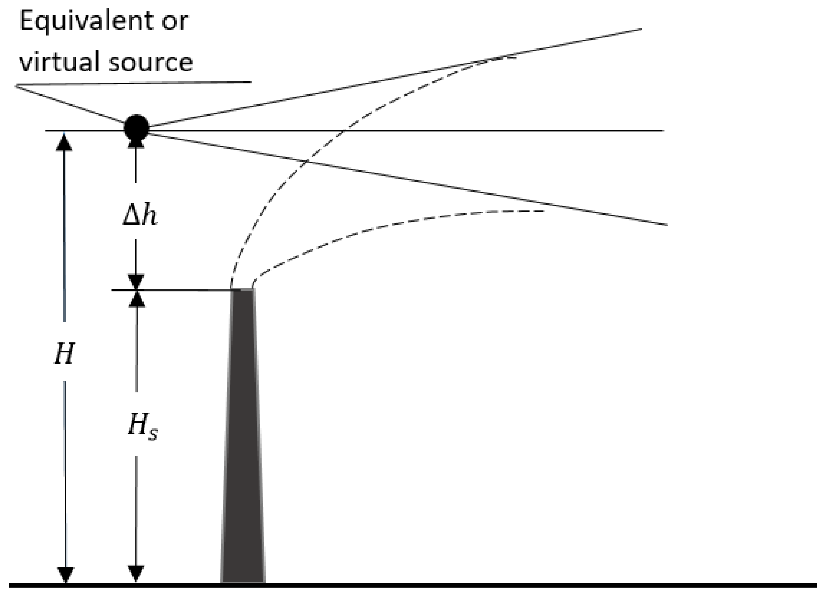
  • Effective height of the point emission source stack. The effective height depends on the velocity of the pollutant released from the stack that can be defined by continuous monitoring. Such monitoring is not in common practice.
  • Emission rate from the stack.
The proposed model reveals the solving of the least square operator for experimental and analytical expression pollutant concentrations, defining emission rate and effective source height as unknown parameters. The standard deviation of the concentration is a subject of new development. It allows the finding of the effective height of the source that depends on unknown emission release velocity from the point source stack. The new model definition requires solving the complex non-linear system of the equations. The solution in such a system is defined by the theory of hypernumbers [5,6,7,8]. The particulate data acquisition uses an Adafruit PM 2.5 sensor. The analog data from the sensor are read by an analog-digital converter. The output from the converter is plugged into a Raspberry Pi 4 B minicomputer to process data. The model evaluation reveals the following steps:
  • Measuring particle concentrations at multiple locations around the plant with the PM 2.5 sensor and storing data in the Raspberry Pi.
  • Computing emission rate, effective emission source stack height and standard deviations of concentration with model using concentrations collected in previous step.
  • Calculating concentrations around the plant with the direct emission dispersion model.
  • Testing the model’s accuracy by comparing concentrations defined in the previous step with the dispersion model and experimental data at the same points, different from those defined in the first step.

2. Inverse Reconstructing Model and Solution with Theory of Hypernumbers

The direct model of pollutant dispersion from the pointed source is:
C x , y , z = Q 2 π 3 / 2 u σ x σ y σ z e x x 0 2 2 σ x 2 e y y 0 2 2 σ y 2 e z H 2 2 σ z 2
Q is the emission strength of the source g/s, u is the average wind speed through the plume–m/s, C is the concentration (g/m3), σ x ,   σ y ,   σ z are horizontal and vertical standard deviations (m), H is the equivalent source height (Figure 1).
The inverse model targets finding unknown parameters. Δ h ,   Q are defined to satisfy:
U = m i n i = 1 N C x i ,   y i , z   Q 2 π 3 / 2 u σ x σ y σ z e x i x 0 2 2 σ x 2 e y i y 0 2 2 σ y 2 e z h s + Δ h 2 2 σ z 2 2
U Δ h = i = 1 N C i x i ,   y i , z   Q 2 π 3 / 2 u σ x σ y σ z e x i x 0 2 2 σ x 2 e y i y 0 2 2 σ y 2 e z h s + Δ h 2 2 σ z 2 2 Q 2 π 3 / 2 u σ x σ y σ z e x i x 0 2 2 σ x 2 e y i y 0 2 2 σ y 2 e z h s + Δ h 2 2 σ z 2 z h s + Δ h = 0
U Q = i = 1 N C i x i ,   y i , z   Q 2 π 3 / 2 u σ x σ y σ z e x i x 0 2 2 σ x 2 e y i y 0 2 2 σ y 2 e z h s + Δ h 2 2 σ z 2 1 2 π 3 / 2 u σ x σ y σ z e x i x 0 2 2 σ x 2 e y i y 0 2 2 σ y 2 e z h s + Δ h 2 2 σ z 2 = 0
The pollutant source characteristics Δ h m   and   Q m are defined as the following hypernumbers:
Δ h m = H n Δ h m m ω
Q m = H n Q m m ω
Δ h m + 1 = Δ h m + δ Δ h m
Q m + 1 = Q m + δ Q m
The hypernumber deviations δ Δ h m and δ Q m are defined from the linear system of the equations
μ U Δ h = δ Δ h m d 11 + δ Q m d 12
μ U Q = δ Δ h m d 21 + δ Q m d 22
The coefficients d i , j are defined with (Equation (11))
d 11 = 2 U Δ h 2   ,     d 12 = 2 U Δ h Q   ,     d 21 = d 12 ,     d 22 = 2 U Q
Using (Equations (3), (4) and (11)) allows us to find coefficients and hypernumber deviations.
d 11 = e z h s + Δ h 2 2 σ z 2 z h s + Δ h 2   σ z 2 + 1 i = 1 N C i x i ,   y i , z   2 π 3 2 u σ x σ y σ z e x i x 0 2 2 σ x 2 e y i y 0 2 2 σ y 2 e z h s + Δ h 2 σ z 2 + e z h s + Δ h 2 σ z 2 2 z h s + Δ h 2   σ z 2 + 1 i = 1 N 2 Q 2 2 π 3 u 2 σ x 2 σ y 2 σ z 2 e x i x 0 2 σ x 2 e y y i y 0 2 σ y 2 e z h s + Δ h 2 σ z 2
d 12 = i = 1 N 4 Q 2 π 3 u 2 σ x 2 σ y 2 σ z 2 e x i x 0 2 σ x 2 e y i y 0 2 σ y 2 e z h s + Δ h 2 σ z 2 z h s + Δ h
d 22 = i = 1 N 2 2 π 3 u 2 σ x 2 σ y 2 σ z 2 e x i x 0 2 σ x 2 e y i y 0 2 σ y 2 e z h s + Δ h 2 σ z 2
Solving the system of the linear equations (Equations (9) and (10)) and plugging Δ h m   and δ Q m into (Equations (7) and (8)) are the calculated hypernumbers solution for the pollution dispersion model.

3. Conclusions

The new solution allows us to define the rate of the pollutant exhaust with high accuracy because the computation is implemented with the effective height of the pollutant output instead of using geometric height. Due to the algorithm’s simplicity, the real time calculation can be done using Raspberry PI or Arduino. Using the new generation of nanotechnological air and water quality sensors and low-cost computational devices would significantly increase the scale of data acquisition and consequently the quality of the environmental quality analysis.

Author Contributions

Conseptualization of inverse mathematics model, A.D.; methodology of data acquisition, P.O.; formal analysis, A.D. and P.O.; writing-original draft preparation, P.O. and A.D.; writing—review and editing A.D and P.O. All authors have read and agreed to the published version of the manuscript.

Funding

This research received no external funding.

Institutional Review Board Statement

Not applicable.

Informed Consent Statement

Not applicable.

Data Availability Statement

Not applicable.

Conflicts of Interest

The authors declare no conflict of interest.

References

  1. Macdonald, R. Theory and Objectives of Air Dispersion Modelling. In Modeling Air Emissions for Complianc; MME 474A Wind Engineering (Course Notes); University of Waterloo: Waterloo, ON, Canada, 2003; 27p. [Google Scholar]
  2. Awastthi, S.; Khare, M.; Gargawa, P. General Plume Dispersion Model (GPDM) for Point Source Emissions. Environ. Model. Assess. 2006, 11, 267–276. [Google Scholar] [CrossRef]
  3. Lushi, E.; Stockie, J. An inverse Gaussian Plume Approach for Estimating Atmospheric Pollutant Emissions from Multiple Point Sources. Atmos. Environ. 2010, 44, 1097–1107. [Google Scholar] [CrossRef] [Green Version]
  4. Seibert, P. Inverse dispersion modelling based on trajectory-derived sourcereceptor relationships. In Air Pollution Modeling and Its Application XII; Gryning, S.E., Chaumerliac, N., Eds.; Plenum: New York, NY, USA, 1997. [Google Scholar]
  5. Burgin, M. Nonlinear partial differential equations in extrafunctions. Integr. Math. Theory Appl. 2010, 2, 17–50. [Google Scholar]
  6. Burgin, M.; Dantsker, A.M.; Esterhuysen, K. Lithium Battery Temperature Prediction. Integr. Math. Theory Appl. 2014, 3, 319–331. [Google Scholar]
  7. Burgin, M.; Dantsker, A. Real-Time Inverse Modeling of Control Systems. In Hypernumbers; Nova Science Publishers: New York, NY, USA, 2015. [Google Scholar]
  8. Burgin, M.; Dantsker, A.M. A Method of Solving of Operator Equations of Mechanics by means of the Theory of Hypernumbers. Not. Acad. Sci. Ukr. 1995, 8, 27–30. [Google Scholar]
Figure 1. Schema of the pollutant dispersion from the pointed source.
Proceedings 81 00145 g001
Publisher’s Note: MDPI stays neutral with regard to jurisdictional claims in published maps and institutional affiliations.

