The Effect of Sample Size on Bivariate Rainfall Frequency Analysis of Extreme Precipitation ^†

Abstract

The objective of this study is to compare univariate and joint bivariate return periods of extreme precipitation that all rely on different probability concepts in selected meteorological stations in Cyprus. Pairs of maximum rainfall depths with corresponding durations are estimated and compared using annual maximum series (AMS) for the complete period of the analysis and 30-year subsets for selected data periods. Marginal distributions of extreme precipitation are examined and used for the estimation of typical design periods. The dependence between extreme rainfall and duration is then assessed by an exploratory data analysis using K-plots and Chi-plots and the consistency of their relationship is quantified by Kendall’s correlation coefficient. Copulas from Archimedean, Elliptical, and Extreme Value families are fitted using a pseudo-likelihood estimation method, evaluated according to the corrected Akaike Information Criterion and verified using both graphical approaches and a goodness-of-fit test based on the Cramér-von Mises statistic. The selected copula functions and the corresponding conditional and joint return periods are calculated and the results are compared with the marginal univariate estimations of each variable. Results highlight the effect of sample size on univariate and bivariate rainfall frequency analysis for hydraulic engineering design practices.

1. Introduction

Rainfall frequency analysis is an important area of hydraulic engineering design, water resources planning, and management. This involves the selection of the variables of interest, the sampling of a sample series and the choice of the most appropriate population distribution. Analysis of extreme rainfall events has conventionally been performed by prespecifying rainfall duration as a filter to abstract annual maximum rainfall depths as the only variable for analysis. However, this univariate approach does not account for dependence between rainfall properties. Rainfall characteristics, such as total depth, duration, and peak intensity exhibit high variability and a multivariate approach should be studied for extreme rainfall analysis.

The interdependency of extreme rainfall characteristics urged scientists and water managers to derive a joint law in order to successfully describe the main characteristics of the observed hydrological events. The first bivariate frequency distributions were generated based to the hypothesis that the variables of interest either have the same marginal probability distribution or that their joint relationship is normally distributed (or becomes normally distributed after a transformation) [1]. In recent years, several studies were focused on finding a method which would assess in the investigation of the statistical behavior of dependent hydrological variables without the need of the assumptions that classical bivariate frequency distributions use. The first paper on copulas in hydrology was published by De Michele and Salvadori [2] and in the next few years several other studies further expanded the theory, such as Favre et al. [3], Salvadori and De Michele [4], Salvadori and De Michele [5], and Genest and Favre [6].

The main concept of the copula approach is that a joint distribution function can be divided into two independent parts, one describing the marginal-univariate behavior and the other is the dependence structure [7,8]. Copulas are the functions that describe the dependence between random variables and, as a result, are able to couple the marginals of these variables into their joint distribution function [9]. The importance of this approach in the field of engineering and water science is noticeable. Copula method offers an efficient way of finding reasonable multivariate estimates for hydrological events that have a certain likelihood of occurrence. These estimates are used as design variables of the hydraulic structures. Design variables are characterized by a return period (recurrence interval) defined as the average time elapsing between two successive realizations of an event whose magnitude exceeds a defined threshold [10,11]. In practice, the selection of a reliable return period is crucial as it is the fundamental parameter in the design of hydraulic structures.

To analyze extreme rainfall events and the effect of sample size on rainfall frequency results, a bivariate analysis is conducted in this study using daily precipitation data from selected meteorological stations in Cyprus. Samples of extreme rainfall events are chosen (using annual maximum rainfall depth with corresponding storm durations) and analyzed using copulas to describe the dependence structures between rainfall variables and to construct their joint distribution for extreme rainfall events. With the marginal distributions selected according to the methodology of traditional univariate analysis, using two different types of extreme rainfall series, a set of copula based bivariate distributions for rainfall peak–storm duration are determined and compared for selected design return periods.

2. Study Area and Rainfall Database

During the last century, remarkable variations and trends were observed in precipitation. Pashiardis [12] published a comprehensive study of rainfall extremes presenting rainfall intensity–duration–frequency (IDF) distribution curves for Cyprus. According to this study, the curves for the period 1971–2007 are more intense and extreme than the curves developed in an earlier study for the period 1931–1970 [13]. The average precipitation of 541 mm in the period from 1901 to 1970 dropped to 463 in the period from 1971 to 2009 [12]. Analysis of precipitation data for Cyprus leads to the conclusion that the mean annual rainfall is decreasing whilst the rainfall intensity of extreme events is increasing. Hence, this study’s primary objective is the application of the copula method and the evaluation of its results to extreme rainfall. To that end, approaches to specify the marginal distribution functions for the study’s rainfall characteristics (rainfall depth and storm duration) are initially applied.

Daily rainfall data for 90 years (October 1920–September 2010) were obtained from three meteorological stations (Limassol, Larnaca and Nicosia), located in the wider area of Cyprus, from the European Climate Assessment and Dataset (ECA&D, www.ecad.eu). The sample size of rainfall extreme characteristics can be a major uncertainty factor when dealing with the estimation of rainfall design values. As a general rule, small sized samples cannot correctly interpret the statistical properties of the population distribution. Hence, in order to evaluate the uncertainty of return period estimation in copula method when small data samples are used, each of the 90-year length time-series were divided into 3 sub-datasets and return periods for both univariate and bivariate models were calculated. The 100-year and 500-year return periods were selected for comparison, as they are often used as design variables in the construction of hydraulic structures.

3. Methodology

This study’s primary objective is the application of the copula method and the evaluation of its results. Figure 1 presents the flow diagram of the methodology and shows the steps for rainfall frequency analysis from the three meteorological stations. The first step is the return period estimation for each variable (depth and storm duration) based on the typical univariate approach. Then, the dependence between the two variables of interest is assessed. This could be done either by visualizing dependence or by the performance of statistical tests. The Chi-plot and K-plot are the most common graphical tools for detecting dependence. The statistical tests of dependence were performed by computing Kendall’s correlation coefficient (Kendall’s tau) and both graphical methods were taken into consideration for better visualization of the results.

After the dependence between the variables was evaluated, copulas from three different families were selected as candidate models. In the present work we considered only bivariate distributions and made use of Archimedean (Gumbel–Hougaard, Clayton, Frank, and Joe), extreme value (Gumbel–Hougaard and Tawn) and elliptical (Normal or Gaussian) models. The maximization of the pseudolikelihood, a generally applicable method which does not have limitations regarding the dependence parameter, was selected for estimating the model’s parameters for this study. The exclusion of non-admissible copulas was based to Cramér-von Mises statistic test, computed using a bootstrap procedure as described in Genest et al. [14]. Graphical tests for a visual description of the copula fitting and complementary analysis were also used. Finally, the (corrected) Akaike Information Criterion (AIC) [15,16], among the non-rejected copulas, determined the most appropriate model.

After the choice of the most efficient copula model, the bivariate distributions needed to be constructed. A copula is a joint distribution function of standard uniform random variables able to connect univariate marginal distribution functions with the multivariate probability distribution, as stated in Sklar Theorem [9], as follows:

Let FXY be a joint distribution function with marginals FX and FY. Then there exists a copula C such that:

F_XY (x, y) = C(F_X (x), F_Y (y)),

(1)

for all reals x, y. If FX, FY are continuous, then C is unique; otherwise, C is uniquely defined on Range (FX) × Range (FY). Conversely, if C is a copula and FX, FY are distribution functions, then FXY given by Equation (1) is a joint distribution function with marginals FX and FY.

After modeling the bivariate distribution, the copula-based return periods were computed. In this study, the bivariate joint (primary) return periods, called OR operator, “∪” (union of events—either of the variables u and v exceed the defined thresholds) and AND operator “$\cap$” (intersection of events–both of the variables u and v exceed the defined thresholds) [5,10], were computed and are defined as follows:

$$T_{u,v}^{OR}=\frac{\mu }{1-C_{u,v}(u,v)},$$

(2)

$$T_{u,v}^{AND}=\frac{\mu }{1-{u-v+C}_{u,v}(u,v)},$$

(3)

where u and v follow a uniform distribution U (0,1). The U denotes FX(X) and V denotes FY(Y) and they were constructed after applying the probability integral transform to X and Y, a transformation which allowed us to simplify our work by using an equivalent set of values which follow the standard uniform distribution.

In comparison to the univariate return periods, the joint bivariate estimates are not unique, but instead, they have infinite combinations of values, described with the level curve. All pairs (u, v) that lie on the same level curve of the copula have the same return period T(p), however, these combinations of values for u and v have various probabilities of occurrence and can have significant differences from one another. For the purposes of the present study the most-likely design realization method [17] was used to select a unique return period. This method introduces a weighting function, which specifies the point over the critical layer with the greatest value of the joint probability density function fxy. It is also known as “typical” critical realization, and is described with the following equation:

$$\left(u,v\right)=\underset{C\left(u,v\right)=t}{\underbrace{argmax}}{f}_{XY}\left(F_x^{-1}\left(u\right),F_Y^{-1}\left(v\right)\right),$$

(4)

where u and v depict the converted via the probability integral transform realizations of the marginal distributions F_X and F_Y of the random variables X and Y. After the identification of the maximization point, the pair (u,v) was used in order for the exceedance probability to be calculated. As a final step, a comparison of the different return periods coming from univariate and bivariate analysis was performed in order to investigate the results of the copula method.

4. Results

4.1. Univariate Analysis

After the selection of extreme events, a univariate rainfall frequency analysis was performed for annual maximum rainfall depths and corresponding storm durations. Different probability models, such as Generalized Extreme Values (GEV), Gumbel (EVI), and Generalized Pareto Distribution (GPD) for peak discharge and GEV, Gamma, Exponential, and Log-normal, were applied to the datasets. The distribution’s parameters were estimated with the help of maximum likelihood method, a method which will be as well used in the copula’s parameters estimation process [18]. Subsequently, the Kolmogorov–Smirnov Goodness-of-Fit and graphical tests were produced to select the distributions that produced an adequate fit to the data. Finally, AIC [15] values, among the non- rejected copulas, determined the most appropriate statistical model. In conclusion, the generalized extreme value distribution (GEV) was selected for modelling annual maximum rainfall depth and storm duration.

Table 1. Results of univariate and bivariate approaches for annual maximum rainfall depths and corresponding storm durations for the complete data period and the 3 sub-periods at Limassol Station.

	1st Data Sample	2nd Data Sample	3rd Data Sample	4th Data Sample
Years	1920-2010	1920-1950	1950-1980	1980-2010
Number of Events	90	30	30	30
Kendall’s tau	0.35	0.33	0.26	0.59
Variable: Rainfall Depth
Sampling Method	AMS	AMS	AMS	AMS
Marginal Distribution	GEV	GEV	GEV	GEV
Distribution Parameters (μ,σ,ξ)	7.79, 3.47, -0.07	8.70, 3.39, -0.19	6.87, 2.82, 0.14	7.74, 3.80, -0.06
Kolmogorov Smirnov Test (p>0.05)	0.7835	0.9878	0.9412	0.8746
Variable: Rainfall Duration
Sampling Method	Corresponding value	Corresponding value	Corresponding value	Corresponding value
Marginal Distribution	GEV	GEV	GEV	GEV
Distribution Parameters (μ,σ,ξ)	5.42, 2.65, -0.02	5.52, 2.89, -0.20	6.12, 2.85, -0.07	4.83, 2.18, 0.10
Kolmogorov Smirnov Test (p>0.05)	0.4212	0.5704	0.5942	0.6988
Copula Model	Gaussian (par = 0.54, tau = 0.36)	Clayton (par=0.81, tau=0.29)	Frank (par=2.34, tau=0.25)	Gumbel (par=2.63, tau=0.62)
Von Mises (bootstrap) (p>0.05)	0.18	0.44	0.97	0.24

presents the results of the univariate approach for the Limassol meteorological station for the complete period of analysis and for the three subperiods. Finally, when the appropriate model was selected, the univariate return periods were calculated for 2, 5, 10, 25, 50, 100, 200, and 500 years.

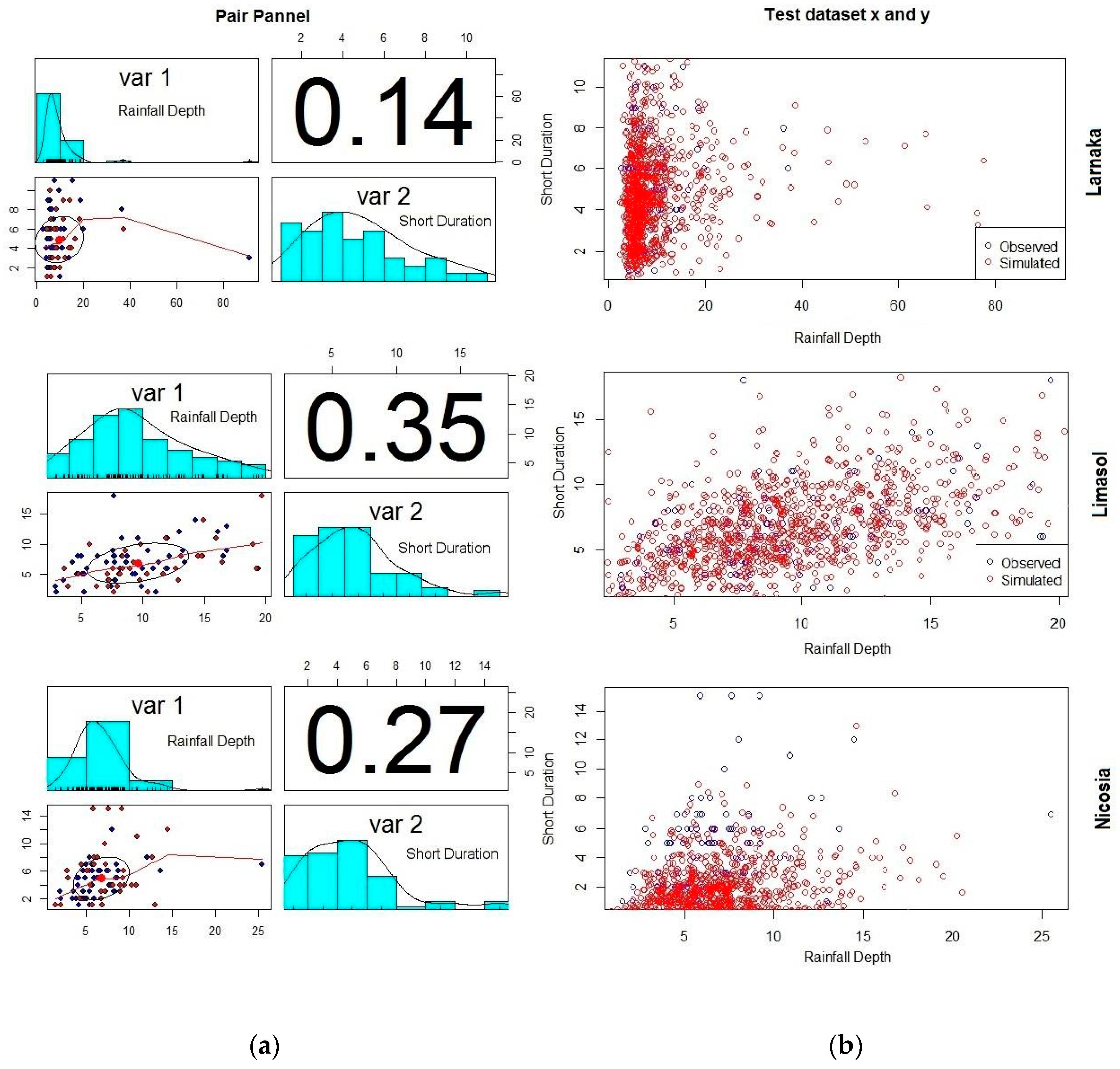
4.2. Bivariate Analysis

After the univariate analysis was performed, a formal assessment of the dependence between the pairs of the considered variables was tested with the help of the Kendall correlation coefficient. Histograms and a scatterplot of the Rainfall Depth (X)-Duration (Y) pair are presented in Figure 2a, in which a weak correlation between the two variables can be easily noticed. In the next step, the different copulas from the three families were fitted to X-Y pairs. The parameters of the copulas were estimated with the maximum pseudolikelihood method and the considered functions were compared with different goodness-of-fit tests. Table 1 shows the best copulas selected for the Limassol meteorological station for all sample periods. For example, for the complete period of analysis (1920–2010) the Gaussian copula with parameter = 0.54 was selected for the AMS sample, as it had the lowest AIC value, and at the same time had an adequate fit. The statistical test p-value was 0.18 for the bootstrapped p-value of the goodness-of-fit test, using the Cramer-von Mises statistic (95% significance level). Furthermore, Figure 2b shows the graphical tests of the selected copulas for a sample size of 1000 simulations for the X-Y pair (Rainfall Depth–Duration). The Kendall‘s tau, extracted from the comparison between observed and simulated values, was 0.36 for the copula and for the actual data, indicating that the correlation of the real data was preserved in the copula. Similar results are observed for the other sub-periods and the other two meteorological stations (Larnaca and Nicosia). It should be mentioned that, in these two stations, lower correlations are observed between annual maximum rainfall depth and corresponding storm durations (Figure 2).

After copula selection, the bivariate distribution function was constructed and the selected marginals were taken into consideration. Figure 3 illustrates the level curves for the bivariate return periods for the Limassol station and the complete data period of 90 years.

Table 2. Results of the Bivariate Return Periods 2, 5, 10, 25, 50, 100, 200 and 500 for Rainfall Depth and Storm Duration—Limassol meteorological station.

Return Level (years):	2	5	10	25	50	100	200	500
Rainfall Depth - dual (cm)	7.58	10.83	13.10	16.65	18.94	20.98	22.70	25.05
Rainfall Depth - cooperative (cm)	10.62	14.20	16.41	19.04	20.88	22.60	24.24	26.79
Rainfall Duration - dual (d)	5.19	7.61	9.12	9.88	10.22	10.50	10.98	11.61
Rainfall Duration - cooperative (d)	7.55	10.47	12.36	14.72	16.45	18.16	19.81	21.60

shows the derived joint return (primary) periods for the OR (union) and AND (intersection) cases, constructed following the Equations 2 and 3 and the most likely realization method, as described in Equation 4. The T^OR and T^AND joint return periods express the possible conditions of failure in case of having two variables which are considered important for design purposes. To be more comprehensive, the variables of interest can either work together or simultaneously in order to cause failure. In case that the condition of failure is met when either or both rainfall depth (X) and rainfall duration (Y) variables exceed their threshold, the cooperative risk T^OR should be taken into consideration. On the other hand, in case that failure occurs when both X and Y variables exceed their threshold simultaneously (or dually), the dual return period T^AND needs to be calculated. The calculation of the two different joint return period cases is important as if the two variables X and Y can cooperate (OR case) then the marginal probabilities must be considerably higher.

The analysis of the samples at Limassol meteorological station showed that GEV distribution is the most appropriate for modeling both duration and rainfall depth. The parameters of the fitted distributions had differences from one another, and at the same time, Kendall’s correlation coefficient indicated that the last thirty years had a much stronger correlation (0.59) than the others (approximately 0.30). The copula models used were different in every sample and can be seen in Table 1. The return periods (not shown due to paper length limitations), have relatively small differences in the 100 year return period, whereas in the 500 year period there were differences in AND and OR cases, with values ranging from 9.94 to 25.05 and 21.74 to 40.05, respectively.

5. Concluding Remarks

In the present study, a bivariate rainfall frequency analysis is performed using an extensive selection of bivariate copulas, as well as different statistical and graphical tests. Annual Maximum Series are followed in order to collect the data samples, and then the corresponding univariate and bivariate return periods are evaluated and compared.

In total, the return periods obtained are in consensus with Salvadori et al. [5] who showed that the relationship between univariate and primary (bivariate) return periods can be written as T^OR < T^UNI < T^AND. The correlation analysis in the two study variables confirms that a slight dependence exists between the extreme rainfall characteristics (rainfall depth and duration). It is worth noting that, even though the correlation pattern changes when different samples are selected, the return period estimates do not have significant differences.

In conclusion, the existence of dependence among hydrological variables indicates the need for multivariate distributions to be constructed, especially when dealing with design values. As a result, more studies should be performed in order to investigate the importance of copula application in rainfall frequency analysis and the effect of sample size in design return periods.

References

1. Zhang, L.; Singh, V.P. Bivariate rainfall frequency distributions using Archimedean copulas. J. Hydrol. 2007, 332, 93–109. [Google Scholar] [CrossRef]
2. De Michele, C.; Salvadori, G. A Generalized Pareto intensity-duration model of storm rainfall exploiting 2-Copulas. J. Geophys. Res.-Atmos. 2003, 108. [Google Scholar] [CrossRef]
3. Favre, A.C.; El Adlouni, S.; Perreault, L.; Thiémonge, N.; Bobée, B. Multivariate hydrological frequency analysis using copulas. Water Resour. Res. 2004, 40, W01101. [Google Scholar] [CrossRef]
4. Salvadori, G.; De Michele, C. Frequency analysis via copulas: theoretical aspects and applications to hydrological events. Water Resour. Res. 2004, 40. [Google Scholar] [CrossRef]
5. Salvadori, G.; De Michele, C.; Kottegoda, N.T.; Rosso, R. Extremes in Nature. In An Approach Using Copulas; Springer: Dordrecht, the Netherlands, 2007; Volume 56, p. 292. [Google Scholar]
6. Genest, C.; Favre, A.C. Everything You Always Wanted to Know about Copula Modeling but Were Afraid to Ask. J. Hydrol. Eng. 2007, 12, 347–368. [Google Scholar] [CrossRef]
7. Juri, A.; Wüthrich, M.V. Copula convergence theorems for tail events. Insur. Math. Econ. 2002, 30, 405–420. [Google Scholar] [CrossRef]
8. Papaioannou, G.S.; Kohnová, T.; Bacigal, J.; Szolgay, K.; Hlavčová, A.; Loukas, A. Joint Modelling of Flood Peaks and Volumes: A Copula Application for the Danube River. J. Hydrol. Hydromech. 2016, 64, 382–392. [Google Scholar] [CrossRef]
9. Sklar, A. Fonctions de répartition à n dimensions et leurs marges. Publ. Inst. Stat. Univ. Paris 1959, 8, 229–231. [Google Scholar]
10. Gräler, B.; Vandenberghe, S.; Petroselli, A.; Grimaldi, S.; Baets, B.D.; Verhoest, N.E.C. Multivariate return periods in hydrology: A critical and practical review focusing on synthetic design hydrograph estimation. Hydrol. Earth Syst. Sci. 2013, 17, 1281–1296. [Google Scholar] [CrossRef]
11. Salvadori, G. Bivariate return periods via 2-copulas. Stat. Methodol 2004, 1, 129–144. [Google Scholar] [CrossRef]
12. Pashiardis, S. Compilation of Rainfall Curves in Cyprus; Meteorological Note No. 15; Meteorological Service, Ministry of Agriculture, Natural Resources and Environment: Nicosia, Cyprus, 2009. [Google Scholar]
13. Hadjiioannou, L. Rainfall Intensities in Cyprus and Return Periods; Meteorological Note No. 16; Meteorological Service, Ministry of Agriculture, Natural Resources and Environment: Nicosia, Cyprus, 1995. [Google Scholar]
14. Genest, C.; Rémillard, B.; Beaudoin, D. Goodness-of-fit tests for copulas: a review and a power study. Insur. Math. Econ. 2009, 44, 199–213. [Google Scholar] [CrossRef]
15. Akaike, H. Information theory and an extension of the maximum likelihood principle. In Second International Symposium on Information Theory; Petrov, B.N., Csaki, F., Eds.; Academiai Kiado: Budapest, Hungary, 1973; pp. 267–281. [Google Scholar]
16. Brunner, M.I.; Favre, A.C.; Seibert, J. Bivariate return periods and their importance for flood peak and volume estimation. Wiley Interdiscip. Rev. Water. 2016, 3, 819–833. [Google Scholar] [CrossRef]
17. Salvadori, G.; De Michele, C.; Durante, F. On the return period and design in a multivariate framework. Hydrol. Earth Syst. Sci. 2011, 15, 3293–3305. [Google Scholar] [CrossRef]
18. Salvadori, G.; Durante, F; Tomasicchio, G.R.; D’Alessandro, F. Practical guidelines for the multivariate assessment of the structural risk in coastal and offshore engineering. Coast Eng. 2014, 95, 77–83. [Google Scholar] [CrossRef]
Figure 1. Flow diagram of the methodology.
Proceedings 07 00019 g001
Figure 2. (a) A scatterplot matrix of the selected variables and their Kendall correlation coefficient for the study meteorological stations; (b) Comparison between the observed and simulated values (sample size 1000) (Rainfall Depth–Duration) for Frank (Larnaca) and Gaussian (Limassol and Nicosia) copulas for 1000 simulations, indicating an adequate fit between the simulating and observed values.
Proceedings 07 00019 g002
Figure 3. Level curves for the bivariate return periods, white for cooperative risk TOR and black for dual risk TAND. The color range changes as the probability reaches from 0 to 1. U denotes FX(X) which represents the random variable from the marginal distribution of the rainfall depth values and V denotes FY(Y) which represents the random variable from the marginal distribution of the storm duration values. Each of the lines refer to a specific return period and the values on the two axes are equivalent to the probabilities of occurrence of the random variables X (annual maximum rainfall depths) and Y (corresponding storm durations), respectively.
Proceedings 07 00019 g003