Abstract
Annual maximum daily rainfalls will change in the future because of climate change, according to climate projections provided by EURO-CORDEX. This study aims at understanding how the expected changes in precipitation extremes will affect the flood behavior in the future. Hydrological modeling is required to characterize the rainfall-runoff process adequately in a changing climate to estimate flood changes. Precipitation and temperature projections given by climate models in the control period usually do not fit the observations in the same period exactly from a statistical point of view. To correct such errors, bias correction methods are used. This paper aims at finding the most adequate bias correction method for both temperature and precipitation projections, minimizing the errors between observed and simulated precipitation and flood frequency curves. Four catchments located in central western Spain have been selected as case studies. The HBV hydrological model has been calibrated, using the observed precipitation, temperature, and streamflow data available at a daily scale. Expected changes in precipitation extremes are usually smoothed by the reduction of soil moisture content due to expected increases in temperatures and decreases in mean annual precipitation. Consequently, rainfall is the most significant input to the model and polynomial quantile mapping is the best bias correction method.
PACS:
J0101
1. Introduction
Climate change is a reality and affects the most dangerous natural hazard in Europe, floods. Because of that, several studies and models have been developed to try to prevent their damages. In Spain, there are two sources of climate projections under climate change supplied by AEMET (‘Agencia Estatatal de Metorología’, in Spanish) and CORDEX. Garijo et al. [1] found that AEMET projections do not adequately characterize extreme events. Consequently, in this study, climate projections supplied by EURO-CORDEX are used. These climate projections denote that annual maximum daily rainfall quantiles will increase in some parts of Spain. Temperature and precipitation time series are the input data of the HBV model, calibrated with the methodology previously proposed [2].
The GCM has a limited capacity to capture climatic variations at the catchment scale. Therefore, the mismatch between general and regional climate models needs to be corrected [3]. In addition, inputs to obtain simulated floods used to design spillways need to be the most similar to observations, in order to obtain accurate predictions in the future. Consequently, bias correction methods will be applied to both temperature and precipitation time series.
2. Methods
The methodology consists of the following steps: (i) calibration of the HBV model to adequately characterize the rainfall-runoff processes in a changing climate; (ii) selection of the best bias correction method for precipitation and temperature time series; and (iii) assessment of the expected changes in flood quantiles in the future caused by climate change. A GEV distribution has been used to obtain flood quantiles for a set of return periods.
2.1. Study Area and Data
Four catchments have been selected as case studies. They are located in the Douro river basin, in the northwest part of Spain (Figure 1). A dam is located at the outlet of each catchment. Consequently, observed data of inflow discharges are not recorded directly, but they can be estimated from observations of mean daily reservoir water levels and dam releases, collected by the Centre for Hydrographic studies of CEDEX.
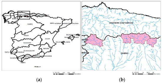
Figure 1.
(a) Location of the case studies in Spain; (b) Catchments of the four case studies.
Time series of daily observations of rainfall and temperature were supplied by the AEMET. Gaps in time series were filled by using observations at nearby gauging stations.
Climate change projections provided by 12 regional climate models of the EURO-CORDEX program have been used (Table 1). Such projections are composed of daily rainfall and temperature time series with a spatial distribution through a grid with cells of 0.11º. The same control period (1971–2004, hydrological years) and future period under climate change (2011–2094, hydrological years) have been considered for all the climate models. The two representative concentration pathways (RCP) considered by the models, RCP 4.5 and 8.5, have been used.

Table 1.
Regional Climate Models used.
2.2. HBV Model and Calibration
The hydrological response in the four catchments has been simulated with the HBV rainfall runoff model [4]. Specifically, the HVB-light-GUI 4.0.0.7 version has been used. The model parameters have been calibrated using Monte Carlo simulations and GAP optimization. Both tools are integrated in the HBV software.
Model parameters have been calibrated using the goodness of fit function ‘Reff’ integrated in the HBV software, which compares the prediction supplied by the model with the simplest possible prediction, a constant value equal to the mean value of observations over the entire period (Equation (1)).
where Qsim(t) is the simulated discharge at time step t, Qobs(t) is the observed discharge at time step t, and is the mean value of discharge observations.
A sensitivity analysis with 1,000,000 Monte Carlo simulations has identified the most important parameters in the four catchments: FC, PERC, K0, and K1. FC is the maximum soil moisture storage. PERC, K0, and K1 are associated with soil infiltration represented by the model with three boxes. As expected, the snow routine is not important in the case studies.
Flood quantiles have been calculated by fitting a Generalized Extreme Value (GEV) distribution to the annual maximum flows simulated by the model. Flood quantiles obtained by the simulation have been compared with flood quantiles obtained from observed data, for a set of return periods. An iteration process has been used, prioritizing the similarity in the simulation of extreme values, because the results of the study will be applied to dam design.
2.3. Bias Correction
Precipitation and temperature projections supplied by climate models in the control period usually do not fit the observations in the same period exactly from a statistical point of view. Such errors could affect simulated flows in future periods. First, temperature and precipitation have been corrected separately. Second, temperature and precipitation correction techniques have been combined to identify the best bias correction methodology. Quantile mapping techniques have been used: QM linear transformation and QM power transformation [5,6] for precipitation series and simple seasonal bias correction for temperature series [6].
3. Results and Discussion
The best bias correction method has been identified for: (i) temperature projections, in terms of monthly averages; (ii) extreme precipitation in climate projections, in terms of frequency curves for annual maximum series; and (iii) extreme simulated discharges.
3.1. Temperature Correction
In the four catchments, monthly mean temperatures supplied by climate models are significantly lower than the observations. The difference between monthly temperatures supplied by each climate model and observations has been added to the temperature time series in each month to correct the bias [6] (Figure 2).
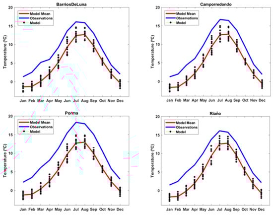
Figure 2.
Comparison of monthly mean temperatures supplied by climate models and observations in the control period. Blue lines are observations. Red lines represent the median of the 12 climate models considered.
3.2. Precipitation Correction
Climate models supply differing precipitation magnitudes in the control period compared to observations. In the Barrios de Luna catchment, climate models supply larger extreme precipitations than observations. However, in the other three catchments, climate models supply lower precipitations.
A set of methods has been considered to correct the errors [6]. In this paper, the Quantile mapping technique has been used, consisting of fitting a function to the comparison of data supplied by the models and observations. Linear and polynomial functions have been considered. The fitted function is used to correct both the control and future data.
The results obtained after correcting bias by the lineal and polynomial techniques show smaller errors than in the case of raw precipitation data. For precipitation frequency curves, the linear correction is the best bias correction method (Figure 3.)
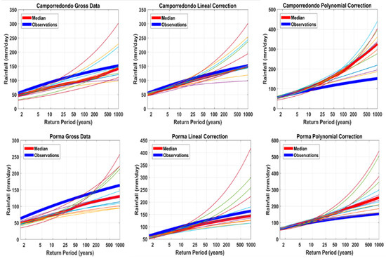
Figure 3.
Frequency curves of annual maximum daily precipitation in two catchments (Camporredondo and Porma). Blue lines are observations. Red lines represent the median of the 12 climate models considered. The first column shows raw precipitation supplied by climate models. The second column shows linear bias correction. The third shows polynomial bias correction. Each row shows a case study.
3.3. Flood Frequency Curves in the Control Period
Simulations of the HBV model have been conducted with a set of combinations of raw and bias corrected temperature and precipitation time series as input data, in order to compare the bias correction techniques. The best bias correction technique is identified in terms of the smallest errors with the flood frequency curve estimated with observations (Figure 4.). The higher return periods have been considered due to their importance in dam design. In general, the smallest errors are obtained with the polynomial bias correction technique. In particular, the methodologies with the smallest absolute error for higher return periods are raw temperature and precipitation supplied by climate models in Barrios de Luna, lineal correction for precipitation and mean monthly temperature correction in Camporredondo, polynomial correction for precipitation and mean monthly temperature correction in Porma, and polynomial correction for precipitation and raw temperature in Riaño.
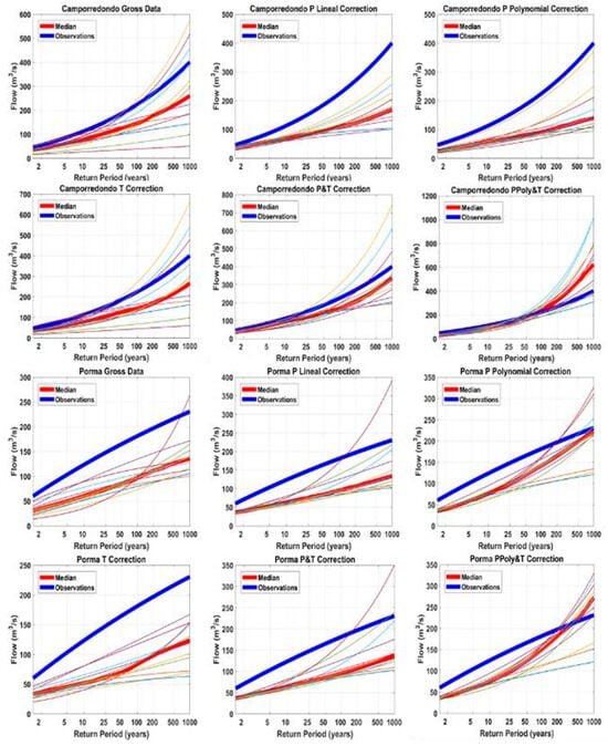
Figure 4.
Comparison of flood frequency curves with observations and HBV simulations using a set of combinations of bias correction techniques in two catchments (Camporredondo and Porma). Blue lines are observations. Red lines represent the median of the 12 climate models considered.
3.4. Flood Frequency Curves in the Future Period
Finally, precipitation and temperature projections in the future (2011–2095) have been obtained in each catchment with the best bias correction techniques identified in the previous step (Figure 5.). Simulations with the HBV model show that, in general, flood frequency curves decrease in the future, though an increase can be seen in some cases.
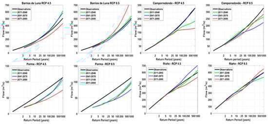
Figure 5.
Flood frequency curves in the future period (2011–2095) with the best bias correction techniques referred to in the previous section.
4. Conclusions
Temperature time series supplied by climate models in the control period are significantly lower than observed data. In addition, bias correction of precipitation time series is more important than temperature correction, affecting flow results.
It has been found that the best bias correction method for precipitation projections, in terms of precipitation frequency curves, differs from the best method in terms of flood frequency curves. Simulations with the HBV model in the future period under climate change assumptions show a general reduction in flood quantiles, smoothing the increases identified in precipitation quantiles. In the control period, when precipitation quantiles are larger than observations, flood quantiles are similar to observations. In general, the period 2071–2095 presents the smallest reductions and, in some cases, larger increases.
In terms of high return periods in flood frequency curves, the best bias correction techniques are the polynomial correction for precipitation and the monthly mean correction for temperature, in the four case studies.
Acknowledgments
The authors acknowledge funding from the Fundación Carlos González Cruz.
Abbreviations
| AEMET | Agencia Española de Meteorología |
| CORDEX | Coordinated Regional Climate Downscaling Experiment |
| GCM | General Climate Model |
| GEV | Generalized extreme value |
| HBV | Hydrologiska Byråns Vattenbalansavdelning |
| QM | Quantile Mapping |
References
- Garijo, C.; Mediero, L.; Garrote, L. Usefulness of AEMET generated climate projections for climate change impact studies on floods at national-scale (Spain). Ingeniería del agua 2018, 22, 153–166. [Google Scholar] [CrossRef]
- Garijo, C.; Mediero, L. Influence of climate change on flood magnitude and seasonality in the Arga River catchment in Spain. Acta Geophys. 2018, 66, 769–790. [Google Scholar] [CrossRef]
- Mehrotra, R.; Sharma, A. A Multivariate Quantile-Matching Bias Correction Approach with Auto- and Cross-Dependence across Multiple Time Scales: Implications for Downscaling. J. Clim. 2016, 29, 3519–3539. [Google Scholar] [CrossRef]
- Seibert, J.; Vis, M. Teaching hydrological modeling with a user-friendly catchment-runoffmodel software package. Hydrol. Earth Syst. Sci. 2012, 16, 3315–3325. [Google Scholar] [CrossRef]
- Shabalova, M.V.; Deursen, W.P.A.; Buishand, TA. Assessing future discharge of the river Rhine using regional climate model integrations and a hydrological model. Clim. Res. 2003, 23, 233–246. [Google Scholar] [CrossRef]
- Teutschbein, C.; Seibert, J. Regional Climate Models for Hydrological Impact Studies at the Catchment Scale: A Review of Recent Modeling Strategies. Geogr. Compass 2010, 4, 834–860. [Google Scholar] [CrossRef]
© 2018 by the authors. Licensee MDPI, Basel, Switzerland. This article is an open access article distributed under the terms and conditions of the Creative Commons Attribution (CC BY) license (https://creativecommons.org/licenses/by/4.0/).