A Model for the Thermal Behaviour of an Offshore Cable Installed in a J-Tube ^†

Abstract

In the race for energy production, supplier companies are concerned by the thermal rating of offshore cables installed in a J-tube, not covered by IEC 60287 standards, and are now looking for solutions to optimize this type of system. This paper presents a numerical model capable of calculating temperature fields of a power transmission cable installed in a J-tube, based on the lumped element method. This model is validated against the existing literature. A sensitivity analysis performed using Sobol indices is then presented in order to understand the impact of the different parameters involved in the heating of the cable. This analysis provides an understanding of the thermal phenomena in the J-tube and paves the way for potential technical and economic solutions to increase the ampacity of offshore cables installed in a J-tube.

1. Introduction

A J-tube is a cylindrical conduit whose role is to protect an energy transmission cable positioned vertically between the seabed and the offshore platform, such as a wind turbine or an oil platform. It takes its name from its J-shape, allowing for better insertion of the cable.

Today, industries using this type of installation are limited by the thermal stresses to which the cable is subjected due to the presence of this tube alone. The IEC 60287 standards [1,2] unfortunately do not take into account this type of configuration. In order to prevent the risk of degradation of the insulating materials inside the cable, Coates proposed in 1988 a de-rating coefficient of 0.87 to be applied to the admissible current (ampacity) [3], based on an experiment. However, this coefficient was questioned as being too severe compared to the real conditions of a J-tube at sea (wind, presence of water).

Some numerical models have been developed to represent an electrical cable in a vertical tube. Hartlein [4] proposes a 1D model, valid in steady state, in parallel with an experimental laboratory model. Anders [5,6] then took this model again, this time considering IEC 60287 standards in order to represent the cable, and to calculate the temperature of the electrical conductor. More recently, Chippendale [7,8] proposes a 2D representation of a J-tube according to three sections: water section, air section and separate electrical phases; then proposes to solve an energy balance like Anders and Hartlein in each of these three sections, linked by mathematical refinement. In particular, he proposes a study of the influence of the upper and lower sections on the emerged tube. You [9] proposes a numerical simulation of an air vent on the cooling of a J-tube, via Fluent, which could be one of the possible technical solutions, although this simulation is not compared with experimental measurements for validation.

Despite the relevance of these studies, none of them proposes a more thorough study of the thermal phenomena that take place within a J-tube. This analysis would be great to identify possible technical solutions for industrials. This article presents this approach. To do so, we will first present an improvement of the permanent 2D model of Chippendale [7,8], which was presented at the international Jicable 2019 congress [10]. It is able to calculate the temperature field at any point in the system, based on the lumped element system. This method proves to be particularly useful for considering a power transmission cable by the IEC 60287 standards, used in work on cables installed in ventilated tunnels [11,12]. This model will be validated by comparison with the results of Chippendale [8]. We will then use this model to perform a sensitivity analysis, based on Sobol indices [13,14,15,16], in order to highlight the parameters having the greatest influence on the thermal stresses of the cable, or on the contrary, to detect parameters whose effect is negligible.

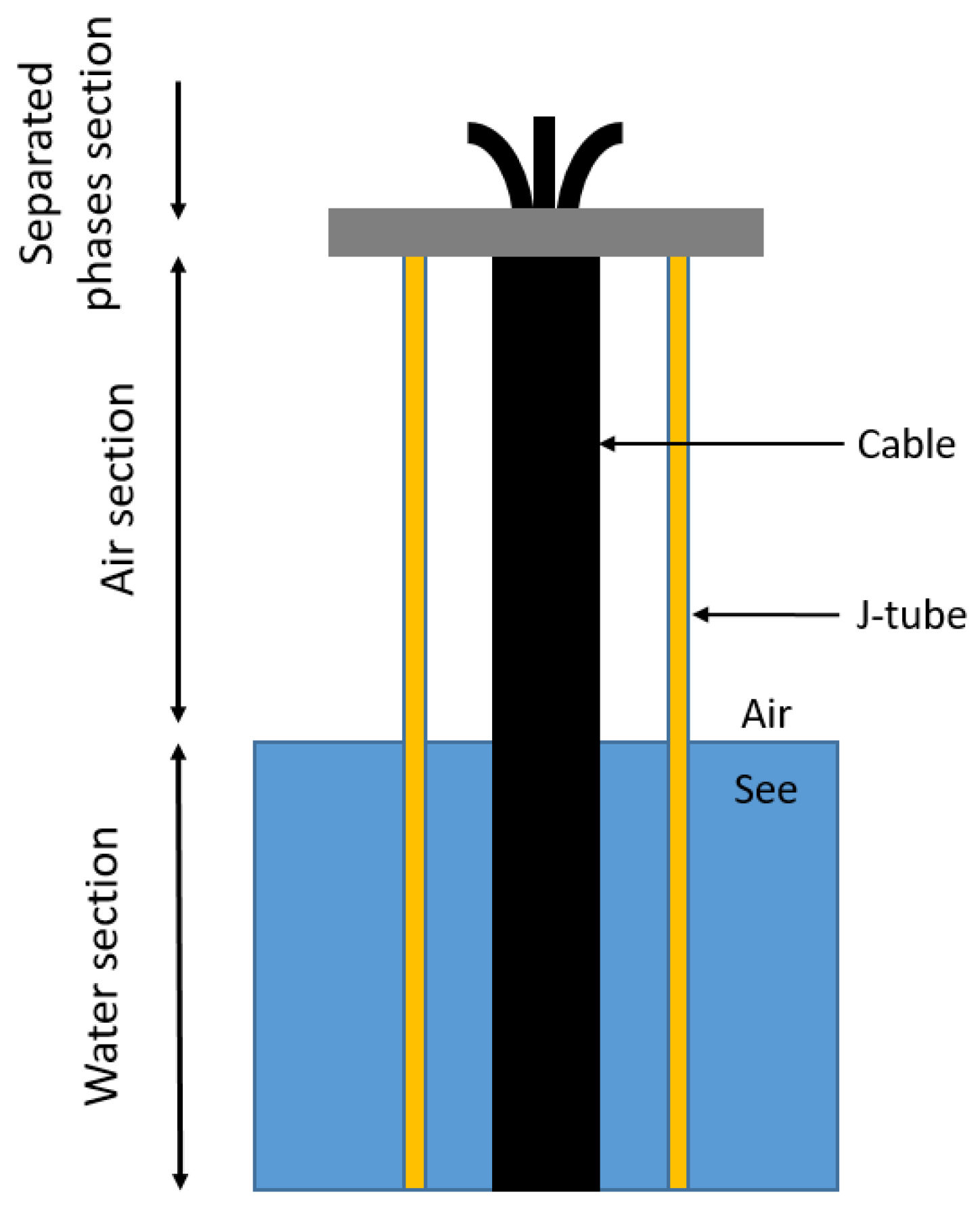
2. Configuration

In order to create a model capable of representing the heat exchanges within it, the configuration can be simplified by considering the cable as centred with the pipe. Moreover, in order to validate our model, we use the representation of Chippendale in [8], and as shown in Figure 1. The system is considered as 2D and is divided into three sections: submerged where the tube encloses the cable with water, emerged with the presence of air between the cable and the tube, and finally the last section where the tube is no longer present and the three-phases cable is divided into its various phases. We also consider that the tube is closed at the top: there is no air exchange between the inside and the outside.

Concerning the cable, we will study a $132 \mathrm{kV}$ SL (Sheath Lead) type cable with a conductor section of $1000 {\mathrm{mm}}^2$, each phase insulated with XLPE. The complete parameters of the electric cable are presented in [8].

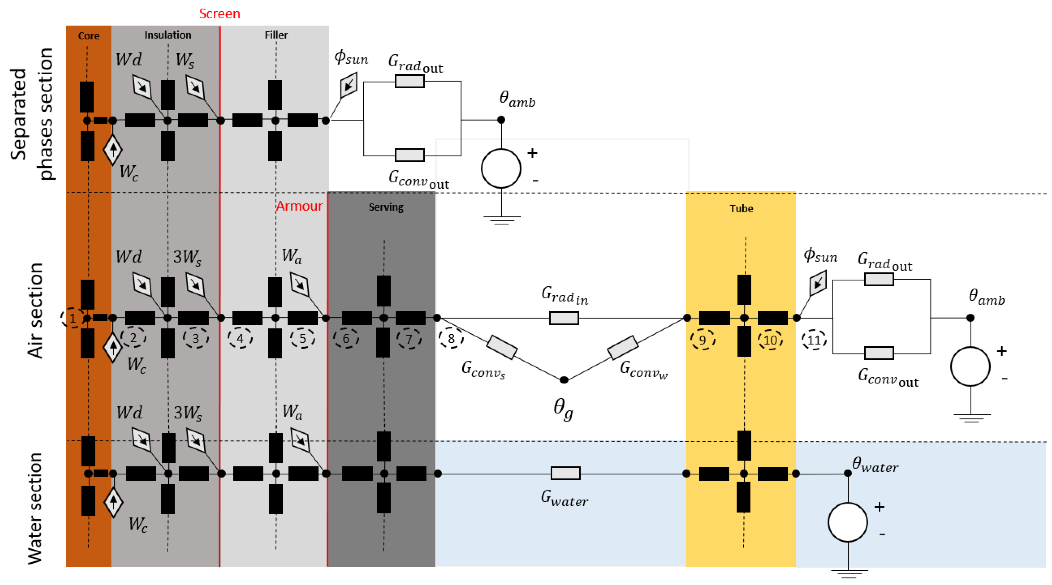
3. Numerical Model

In the case of offshore power cables, it is necessary to find a model that can take into account the electrical analogy imagined in IEC 60287 [1,2,17]. Moreover, this model must remain relatively simple so that it meets user requirements, especially in terms of speed of calculation time, through approximations: calculation of the exchange coefficient between the cable and the tube by correlation, a problem considered as 2D axisymmetric.

This is why this work turned to the lumped element method (also called the nodal method), which is a generalization of the electrical analogy. It will allow us a great flexibility with regard to the thermal behavior of our system thanks to the spatial discretization of the domain. This model could be used in particular in the case of energy transmission cables in ventilated tunnels [11,12]. This part aims to explain the concept of this method and its application on a cable installed in a J-tube.

3.1. Explanations

The nodal method consists of spatially discretizing a domain into several elementary volumes of isotherms. To each isothermal volume $V_i$ is associated a node, representing in steady state a temperature considered as constant. The heat flows (conduction, convection or radiation) between two nodes, $i$ and $j$, passes through a thermal conductance $G_{ij},$ whose expression depends on the volume considered. Finally, source terms can be implemented at certain nodes to represent the heat generation at these same points.

A system of algebraic equations can then be set up. By analogy with electrokinetics, we can interpret this set of nodes as a network allowing us to compute the temperature field at any point in the domain, either in 1D, 2D or 3D.

We can then carry out an energy balance on each of the nodes. If we take into account the transfer modes mentioned above with the neighboring nodes, and the heat sources generated in certain elements, we obtain for an elementary volume $V_i$, in steady state, the Equation (1)

$$0={{\displaystyle \sum }}_j\left({\Phi }_{ij}^{cond}+{\Phi }_{ij}^{conv}+{\Phi }_{ij}^{rad}\right)+q_i{V}_i$$

(1)

with:

• ${\Phi }_{ij}^{cond}, {\Phi }_{ij}^{conv},{\Phi }_{ij}^{rad}$ the net heat inflows into the elemental volume
• $q_i$, the volume density of energy generated and dissipated in the elemental volume $V_i$.

3.2. Application

We can now apply this discretization to our case study. In order to validate the model, we will place ourselves under the same conditions as the previous work [7,8]. More information about this model is available in [10].

3.2.1. Discretization

The discretization scheme of Chippendale’s case is shown in Figure 2. Using the IEC 60287 standards, the cable is modelled as such: a conductive element, considered here as the centre of the cable; an electrical insulation, represented by the thermal resistance $T_1$; a filler, $T_2$; a protective sheath surrounding the cable,$T_3$.

Concerning the screens and the armour, they are very good thermal conductors compared to the elements surrounding them. We can consider them in our thermal model as infinitely thin. The calculation of the thermal resistances $T_1,T_2,T_3$ as well as the electrical losses ${\lambda }_1,{\lambda }_2$ considered here as thermal sources, will be made in the respect of the IEC 60287 standards for this type of cable.

In the standards, only the center of the electrical insulation was subject to an energy balance, in order to take into account the dielectric losses $W_d$. Our model goes further by positioning a node in each of the solid elements. This will allow us to model the heat transfer by conduction in the longitudinal axis at the same time. Finally, contrary to previous work [11,12], it is here extremely important to place a node in the conductive element of the cable, in order to model the influence of the different sections between them. Indeed, most of the materials used in the cable design are poor thermal conductors (insulation, filler, sheath etc.). It is then easily conceivable that the model developed for cables installed in a ventilated tunnel greatly underestimates the heat transfer in the longitudinal axis.

Concerning the environment outside the cable, the nodal model will be modified according to three configurations, respecting the work of Chippendale [7,8].

In the immersed section, the water in the tube is considered as a solid, due to its good thermal conductivity ${\lambda }_{water}$. The thermal linear flux ${\phi }_{water}$ (${\mathrm{Wm}}^{-1}$) is written in the Equation (2). The outside temperature of the tube surface ${\theta }_o$ is considered equal to the surrounding water, i.e., $10 °\mathrm{C}.$

$${\phi }_{water}=\frac{2\pi {\lambda }_{water}}{\log \left(\frac{D_w}{D_s}\right)}\left({\theta }_s-{\theta }_w\right)$$

(2)

In the middle section, the tube encloses the cable with air. Because this gas has a very low thermal conductivity, the exchanges will then take place mainly by thermal radiation and natural convection. When exchanges by radiation involve only surface temperatures of the cable and the J-tube (3) and (4), the natural convection introduces the gas temperature ${\theta }_g$ between the two walls (5) and (6). First of all, by definition of Newton’s law, the convective flow characterized by the exchange coefficient $h_i$ results in the heat exchange between a wall and the ambient fluid. In [8], $h_i$ is calculated from the correlation of the form (7) from [18].

$${\phi }_{ra{d}_{in}}=4F_{sw}\sigma A_s{\theta }_{m_{in}}^3\left({\theta }_s-{\theta }_w\right)$$

(3)

$$F_{sw}=\frac{1}{1+\frac{1-{\epsilon }_s}{{\epsilon }_s}+\frac{A_s}{A_w}\frac{1-{\epsilon }_w}{{\epsilon }_w}}$$

(4)

$${\phi }_{con{v}_s}=h_{conv}{A}_s\left({\theta }_s-{\theta }_g\right)$$

(5)

$${\phi }_{con{v}_w}=h_{conv}{A}_w\left({\theta }_g-{\theta }_w\right)$$

(6)

$$h_{conv}=0.188\frac{{\lambda }_{air}}{Gap} R{a}^{0.322}{H}^{-0.238}{K}^{-0.442}$$

(7)

Similarly to the solid elements constituting the cable, a node is placed in the centre of the pipe in the water and air sections, in order to model its evolution over its length.

On the outer surface of the tube, we consider that the tube is subjected to the solar flux (8). As proposed in [5,8], only half of the surface is influenced by shading. Moreover, the tube is a non-black body, i.e., its absorptivity varies according to the incident ray’s wavelength. Therefore we take a radiative absorption coefficient $\alpha =0.4$ in the calculation of the flux from the Sun, as in [6,7,8]. In the model, it is considered that the Sun emits $H_{sun}=1000 {\mathrm{Wm}}^{-2}$, which corresponds to the solar radiation on a flat plate placed orthogonally to the rays.

$${\varphi }_{sun}=0.5\alpha H_{sun}{A}_o$$

(8)

Finally, in the last section, the phases of the cable are separated so that they can be connected to the platform. In our model, the armour and the sheath surrounding the cable disappear. We consider that the environment acts directly on the outer surface of a phase, corresponding to the outer diameter of the filler $T_2$. The same external conditions as for the emerged section will be applied to this surface.

$${\phi }_{rad}{}_{out}=4\sigma A_o{\theta }_{m_{out}}^3\left({\theta }_o-{\theta }_{amb}\right)$$

(9)

$${\phi }_{con{v}_o}=h_o{A}_o\left({\theta }_o-{\theta }_{amb}\right)$$

(10)

$$h_n=0.021\frac{{\lambda }_{air}}{L_{section}}R{a}_{L_{section}}^{0.4}$$

(11)

In addition, the outer surface of the tube exchanges radiation and convection with the surrounding environment. This then involves a new node ${\theta }_{amb}$ the outside temperature, which is constant. In [8], the wind speed $V_{wind}$ is considered as null. Convection is then only natural. The correlation used is written in the Equation (11).

3.2.2. Calculations

By performing an energy balance at the 11 nodes set up on the radial axis, at the height $k$, we then obtain the following system of 11 equations, based on Figure 2, for the air section. A similar set of equations, not detailed here, is derived for the separated phases section and for the water section.

$$0=G_{12}\left({\theta }_{2,k}-{\theta }_{1,k}\right)+H_{Core}\left({\theta }_{1,k+1}+{\theta }_{1,k-1}-2{\theta }_{1,k}\right)$$

(12)

$$0=G_{12}\left({\theta }_{1,k}-{\theta }_{2,k}\right)+G_{23}\left({\theta }_{3,k}-{\theta }_{2,k}\right)+W_c$$

(13)

$$0=G_{23}\left({\theta }_{2,k}-{\theta }_{3,k}\right)+G_{34}\left({\theta }_{4,k}-{\theta }_{3,k}\right)+H_{Insul}\left({\theta }_{3,k+1}+{\theta }_{3,k-1}-2{\theta }_{3,k}\right)+W_d$$

(14)

$$0=3G_{34}\left({\theta }_{3,k}-{\theta }_{4,k}\right)+G_{45}\left({\theta }_{5,k}-{\theta }_{4,k}\right)+3W_s$$

(15)

$$0=G_{45}\left({\theta }_{4,k}-{\theta }_{5,k}\right)+G_{56}\left({\theta }_{6,k}-{\theta }_{5,k}\right)+H_{Filler}\left({\theta }_{5,k+1}+{\theta }_{5,k-1}-2{\theta }_{5,k}\right)$$

(16)

$$0=G_{56}\left({\theta }_{5,k}-{\theta }_{6,k}\right)+G_{67}\left({\theta }_{7,k}-{\theta }_{6,k}\right)+W_a$$

(17)

$$0=G_{67}\left({\theta }_{6,k}-{\theta }_{7,k}\right)+G_{78}\left({\theta }_{8,k}-{\theta }_{7,k}\right)+H_{Serv}\left({\theta }_{7,k+1}+{\theta }_{7,k-1}-2{\theta }_{7,k}\right)$$

(18)

$$0=G_{78}\left({\theta }_{7,k}-{\theta }_{8,k}\right)+G_{ra{d}_{in}}\left({\theta }_{9,k}-{\theta }_{8,k}\right)+G_{Con{v}_s}\left({\theta }_{g,k}-{\theta }_{8,k}\right)$$

(19)

$$0=G_{910}\left({\theta }_{10,k}-{\theta }_{9,k}\right)+G_{rad}\left({\theta }_{8,k}-{\theta }_{9,k}\right)+G_{Con{v}_w}\left({\theta }_{g,k}-{\theta }_{9,k}\right)$$

(20)

$$0=G_{910}\left({\theta }_{9,k}-{\theta }_{10,k}\right)+G_{1011}\left({\theta }_{11,k}-{\theta }_{10,k}\right)+H_{Tube}\left({\theta }_{10,k+1}+{\theta }_{10,k-1}-2{\theta }_{10,k}\right)$$

(21)

$$0=G_{1011}\left({\theta }_{10,k}-{\theta }_{11,k}\right)+\left(G_{ra{d}_{out}}+G_{Con{v}_{out}}\right)\left({\theta }_{amb,k}-{\theta }_{11,k}\right)+{\varphi }_{sun}$$

(22)

The thermal conductances $G_{ij}$ are characteristic of the conduction taking place within the solid elements, between two nodes located on the radial axis, and are expressed in ${\mathrm{WK}}^{-1}$. They involve the space step $dz$, characteristic of the distance between two nodes on the longitudinal axis. The conductances in the electrical conductor are expressed as $G_{12}$, while the other conductances will be the inverse of the thermal resistances presented by the IEC 60287 standards [1,2] $G_{i{j}_{IEC}}$. A node is placed in the middle of each of the elements $T_2,T_3$, and not only within the electrical insulation $T_1$. We take the same representation of the thermal resistance of IEC 60287, simply dividing it by two (24).

$$G_{12}=\frac{2\pi {\lambda }_{core}dz}{log\left(\frac{r_{core}}{r_{core}/2}\right)}$$

(23)

$$G_{ij}{}_{IEC}=\frac{2dz}{T_{n_{IEC}}}$$

(24)

Concerning the axial conductances $H_i$, present only in the solid parts of the system (cable and tube), we can write them as follows (24), the index i representing the central node to the solids and $r_i$ the corresponding radius from the centre of one core:

$$H_i=\frac{{\lambda }_i\pi \left(r_{i+1}^2-r_{i-1}^2\right) }{dz}$$

(25)

It is then possible to reduce these 11 equations into one (26). We can then solve this equation by iterating on the height $k$ in order to determine $\theta$ (27), the temperature matrix, with in row the radial nodes and in columns the axial nodes. ${\theta }_k$ representing the column of $\theta$ of index $k$.

$$0=\left(G_k-A_k-G_{amb}{}_k-2H_k\right).{\theta }_k+A_k.{\theta }_{ga{s}_k}+G_{amb}{}_k.{\theta }_{amb}{}_k+H_k.\left({\theta }_{k+1}+{\theta }_{k-1}\right)+{\varphi }_k$$

(26)

$$\theta =\left(\begin{array}{ccc}{\theta }_{1,1}& \cdots & {\theta }_{1,nk}\\ ⋮& \ddots & ⋮\\ {\theta }_{11,1}& \cdots & {\theta }_{11,nk}\end{array}\right)$$

(27)

Furthermore, $G_k$ is the matrix of thermal conductances between all nodes positioned on a radial axis. This matrix, of the form presented in Equation (28), is tri-diagonal. It is nevertheless, in this case, not symmetrical because of the presence of the three phases: $3G_{34}$ (14). It also takes into account the radiative conductance $G_{ra{d}_{in}}$ which translates the exchanges by radiation between the cable and the tube.

$$G_k=\left(\begin{array}{ccc}-{\displaystyle {\displaystyle \sum }_j}{G}_{\left(i-1\right)j}& G_{\left(i-1\right)\left(j+1\right)}& 0\\ G_{i\left(j-1\right)}& -{\displaystyle {\displaystyle \sum }_j}{G}_{ij}& G_{i\left(j+1\right)}\\ 0& G_{\left(i+1\right)\left(j-1\right)}& -{\displaystyle {\displaystyle \sum }_j}{G}_{\left(i+1\right)j}\end{array}\right)$$

(28)

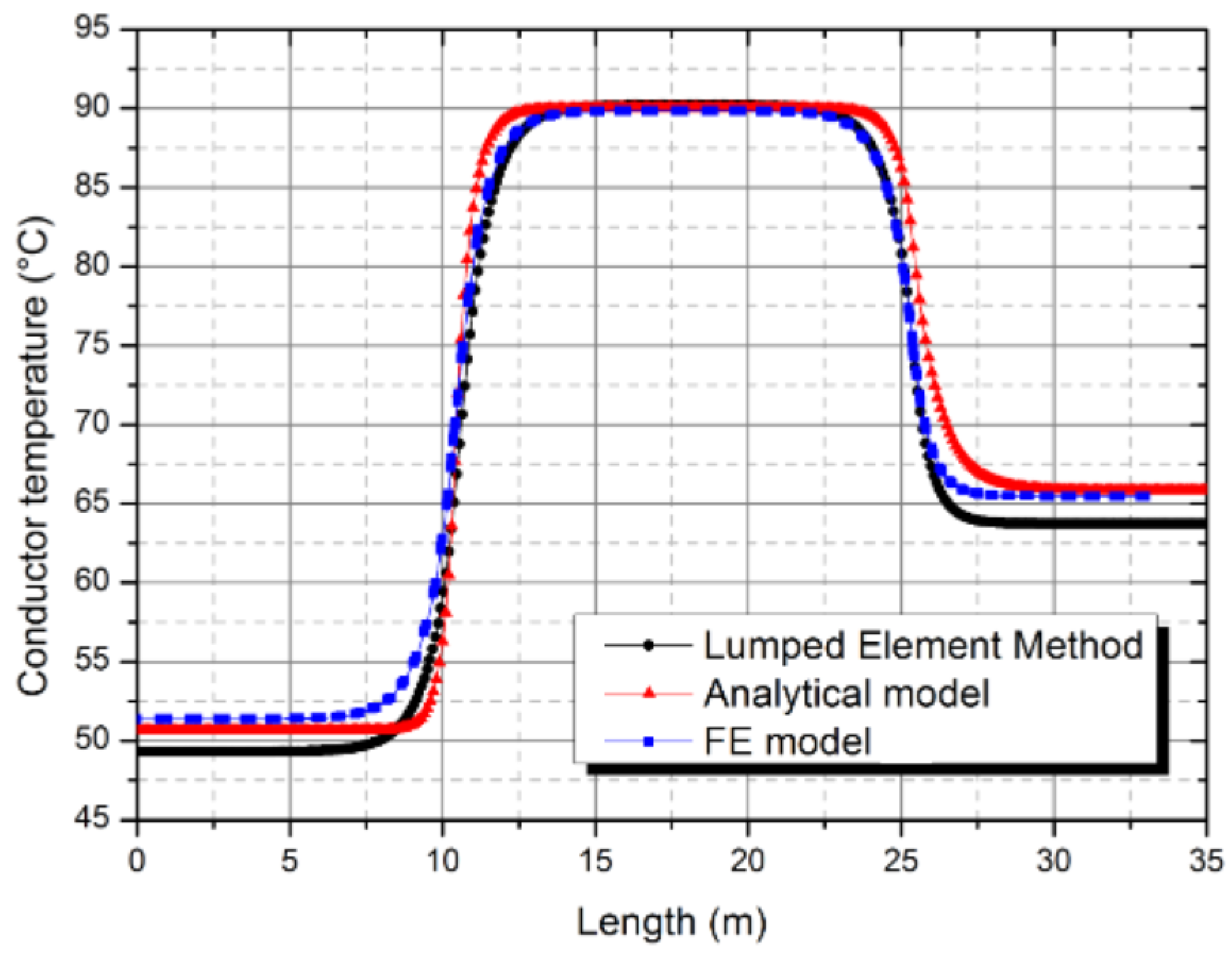
3.2.3. Comparison with Previous Work

Once our model was functional, we compared it to the results obtained by Chippendale in his article [8], taking care to use the same parameterization.

Temperature differences on the water section and separate phases section were most certainly due to the inaccuracies of assumptions made with [8]. However, we can affirm that the good concordance of the results allows us to validate our model.

Moreover, it is important to note that the use of the nodal method in this configuration allows us to connect, by discretization, the three sections imagined by [8], whereas in their work, these transitions are calculated by mathematical extrapolation. It is then quite possible, by this method, to implement in the model a parameterization varying with the height, such as the temperature stratification or the evolution of natural convection towards turbulent regimes.

4. Sensibility Analysis

Now that we have a validated model, it is now interesting to know the parameters whose influences are major or on the contrary negligible. This study thus allows us to understand in detail the influence of each parameter on the thermal stresses that a cable undergoes in a J-tube. From this study, it will be possible to define the elements requiring particular attention in order to improve the cable ampacity as much as possible. In the same way, this study opens the way to future technical solutions that can be envisaged for companies.

4.1. Definition of Study Parameters

The selection of the parameters to be studied through this analysis must follow a certain criterion: to master the interval domain of each parameter. Thus, we will not select the elements for which we do not know the possible variations (elements constituting the cable, skin effect, proximity effect, etc...). The chosen parameters are presented in

Table 1. Studied parameters for sensibility analysis.

Parameters	Min	Max	Unity
Gap	0.05	0.40	m
${\epsilon }_{cable}$	0.4	1	/
${\epsilon }_{Tub{e}_{int}}$	0.4	1	/
${\epsilon }_{Tub{e}_{out} }$	0.4	1	/
$\alpha$$({\alpha }_{tub{e}_{out}}$)	0.2	0.8	/
$h_{conv}$	2	10	$W{m}^2{K}^{-1}$
${\varphi }_{sun}$	0	1000	$W.m^{-2}$
${\theta }_{amb}$	10	50	$°C$
$V_{wind}$	0	10	$m.s^{-1}$

.

To carry out this sensitivity study, we will focus on the maximum temperature obtained by the nodal method (Figure 3), corresponding to one of the electrical conductors of the cable, halfway up the air section. This temperature defines the ampacity of the cable, it is therefore appropriate to study its sensibility. We will then observe its variation according to the study parameters. In order to speed up the calculation time, we change our 2D model to 1D. To do so, we keep only the calculation in air section (Equation (26)), by removing the dependencies according to the height $k$and the matrix of longitudinal conductances $H_k$ from the reduced equation.

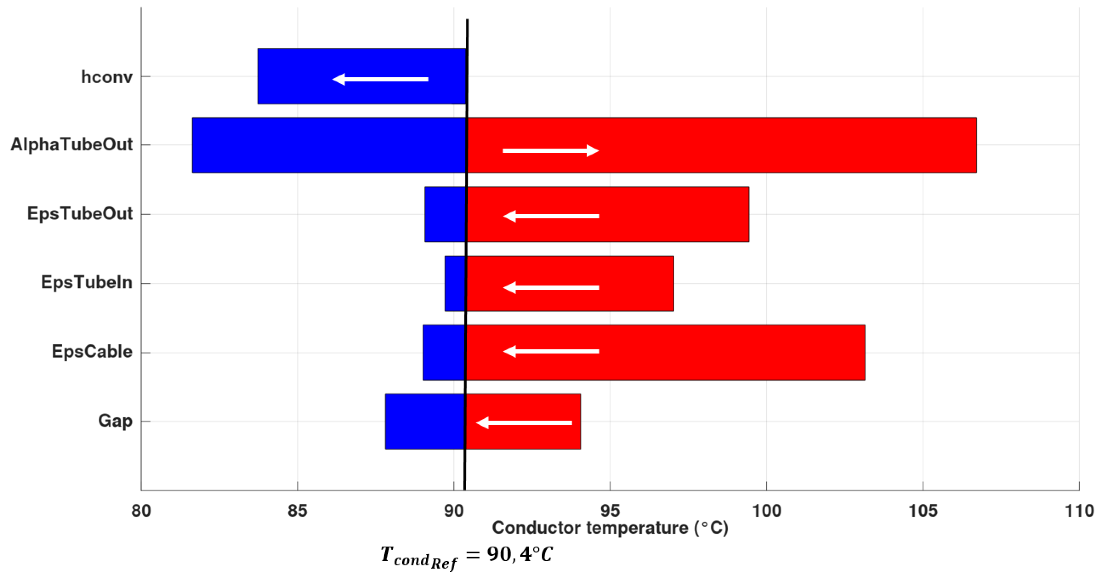
4.2. Simple Parametric Study: “One-at-a-Time”

We can first study the influence of each parameter individually on the output temperature, one by one, by setting all other parameters to a reference. This is an archaic technique, but it is still quite efficient. It is called One-at-a-Time (OAT). It allows a first feedback of the influence of the parameters on the model and its output.

For this OAT analysis, we focus on non-meteorological parameters only. Indeed, these ones cannot be controlled, it is therefore appropriate to not consider them for this first analysis. However, they will be studied in the next section because of their “interactions” effect on the mathematical model. This term will be explained at the end of this section. Furthermore, we decide to study $h_{conv}$ in order to observe the natural convection influence on the cable temperature. There is reason to believe that convection inside an enclosed J-tube is much more complex than a simple correlation (7): temperature stratification, turbulences, air leaks etc. Therefore, an arbitrary exchange coefficient $h_{conv}$ from $2 {\mathrm{Wm}}^{-2}{\mathrm{K}}^{-1}$ to $10 {\mathrm{Wm}}^{-2}{\mathrm{K}}^{-1}$(natural convection range) is considered in this first OAT analysis.

Figure 4 shows the results of this OAT analysis. For each parameter evolving on their range that we have defined in the Table 1, we obtain the evolution of the temperature for each case. Each arrow represents the increasing evolution of the studied parameter. We have also placed on this figure, the temperature value of the reference conductor obtained in Figure 3, as determined in [8].

From this graph, we can draw some conclusions:

• An increase in the gap between the cable and the tube would improve the ampacity of the cable. It is clear that increasing the gap would improve exchanges by natural convection in particular.
• The conductor’s temperature is minimal when the emissivities $\epsilon$ of the surfaces are maximal. However, it should be noted that lower surface emissivity also leads to much higher temperatures. It would therefore be important to precisely characterize these emissivities.
• The influence of the Sun is extremely important here, and modifying the outer surface of the tube to allow it to reflect the Sun’s rays as much as possible would considerably increase the ampacity of the cable.
• Better exchanges by convection inside the tube would undeniably allow better cooling of the cable. Here we have limited ourselves to natural convection ($2 {\mathrm{Wm}}^{-2}{\mathrm{K}}^{-1}<h_{int}<10 {\mathrm{Wm}}^{-2}{\mathrm{K}}^{-1})$, but it is obvious that allowing forced convection, by creating air circulation for example, would greatly improve the ampacity of the cable [9].
• Additionally, it would be interesting to know how important the improvement of the cable temperature could be if we had the ideal configuration, as $\mathrm{p}=0.4\mathrm{m};{\mathsf{\epsilon }}_{\mathrm{cable}}=1;{\mathsf{\epsilon }}_{{\mathrm{tube}}_{\mathrm{int}}}=1;{\mathsf{\epsilon }}_{{\mathrm{tube}}_{\mathrm{out}}}=1;\mathsf{\alpha }=0.2$. For this configuration, we obtain a core temperature of $80.16°\mathrm{C}$, which is an improvement of $11.3\%$ compare to the temperature obtained with the configuration described in [8]. It is important to note that $\mathsf{\alpha }$ is the most influential here: for the configuration $\mathrm{Gap}=0.4\mathrm{m};{\mathsf{\epsilon }}_{\mathrm{cable}}=1;{\mathsf{\epsilon }}_{{\mathrm{tube}}_{\mathrm{int}}}=1;{\mathsf{\epsilon }}_{{\mathrm{tube}}_{\mathrm{out}}}=1;\mathsf{\alpha }=0.4$, we obtain a core temperature of $87.57°\mathrm{C}$ i.e., a $3.1\%$ improvement.

This study by OAT allowed us to understand the influence of each parameter on the temperature of the conductor in the emerged section. However, it turns out that each of these variations was obtained by setting all the other parameters to fixed values. This has the consequence of masking the interaction effects between the parameters in the model: ${\beta }_{1}x {\beta }_2$. In other words, the effects observed in Figure 4 may be different if another reference is chosen.

4.3. Sobol Indices

We must then find a method to obtain the influence of each parameter on the model, while considering the interactions between each parameter: this is a so-called global analysis, as opposed to the OAT which is a local analysis. In addition, we have at our disposal a fast model in resolution time. That is why we turned to the Sobol Indices.

4.3.1. Explanation

Let our model be such that $X_1, X_2,\dots ,X_p$ are the input parameters and $Y$ is its output value. In order to appreciate the influence of the parameter $X_i$ on $Y$, it is possible to study the value of the variance of $Y$according to $X_i$, $V(E[Y|X_i])$. Thus, this quantity will be more important as the variable $X_i$ will be important vis-à-vis the variance of Y, V(Y). In order to use a normalized indicator, we can define the sensitivity index of Y according to $X_i$:

$$S_i=\frac{V\left(E\left[Y|X_i\right]\right)}{V\left(Y\right)}<1$$

(29)

This index is called the first order sensitivity index by Sobol [14]. It quantifies the sensitivity of Y relatively to $X_i$, or the portion of variance of Y due to the variable $X_i$ alone.

In order to consider the interaction effects between variables, let us introduce the variance decomposition theorem, which expresses the fact that the total variance of Y is the sum of the main effects of each variable $V_i$ and the interaction terms $V_{ij}, V_{ijk}$.

$$V\left(Y\right)={\displaystyle \sum }_{i=1}^p{V}_i+{\displaystyle \sum }_{1<i\ne j<p}{V}_{ij}+\dots +{{\displaystyle \sum }}^{\text{}}{V}_{i\dots p}$$

(30)

Thus, from this decomposition, it is then possible to calculate the sensitivity indices of order two $\frac{V_{ij}}{V}$, order three $\frac{V_{ijk}}{V}$, etc. The interpretation of these indices is relatively easy: their sum is equal to one and the larger the index (close to one), the greater the influence of the variable. However, when the number $p$of variables becomes too large, it is difficult to estimate all sensitivity indices. Homma and Saltelli [19] then introduce a total sensitivity index which expresses the total sensitivity of the variance of Y according to $X_i$ (sensitivity to the variable alone and to the interactions of this same variable with the other variables). From the variance decomposition previously presented (30), we can express the total sensitivity index as:

$$S_{T_i}=1-\frac{V\left(E\left[Y|X_{~i}\right]\right)}{V\left(Y\right)}$$

(31)

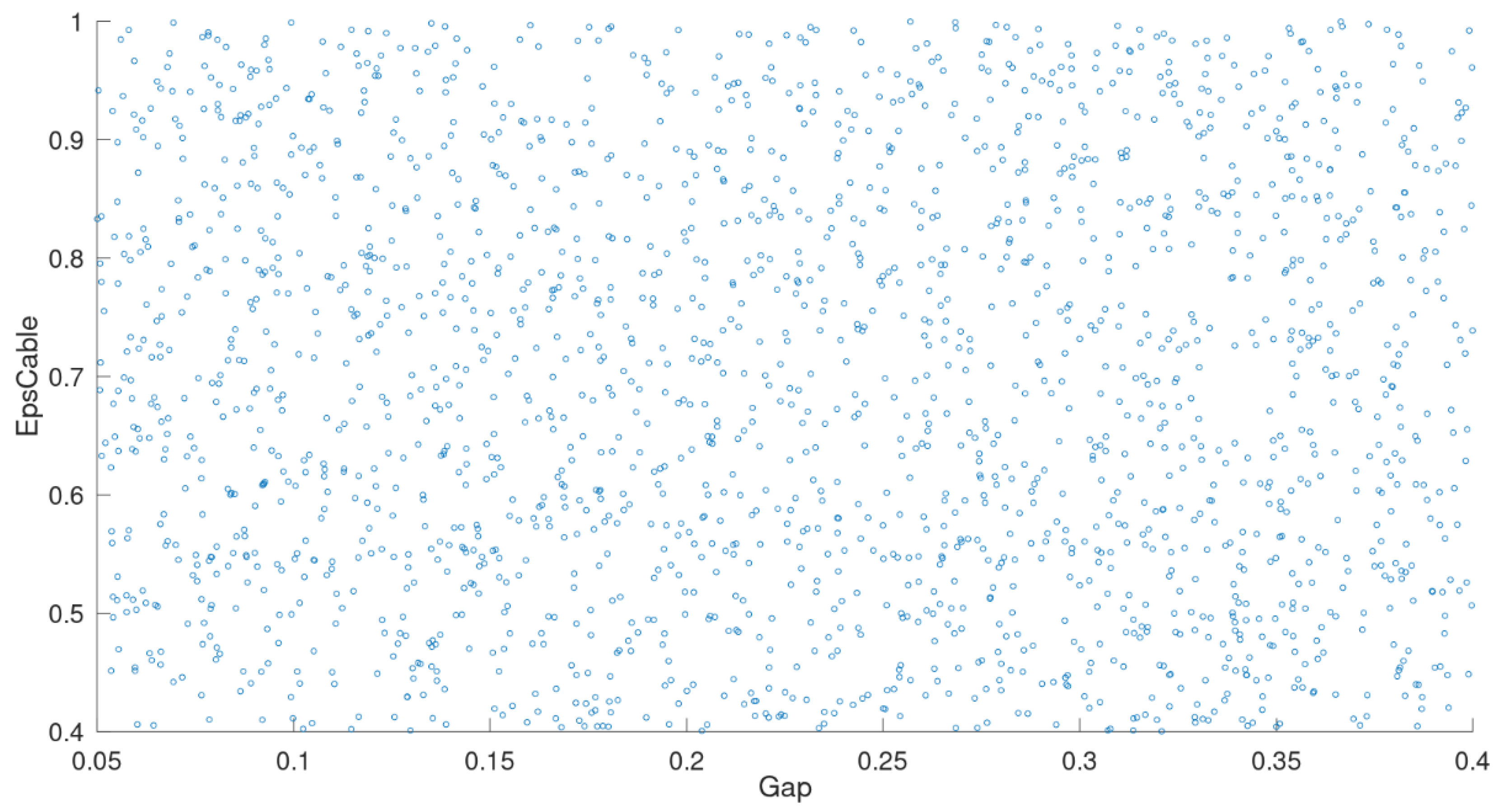
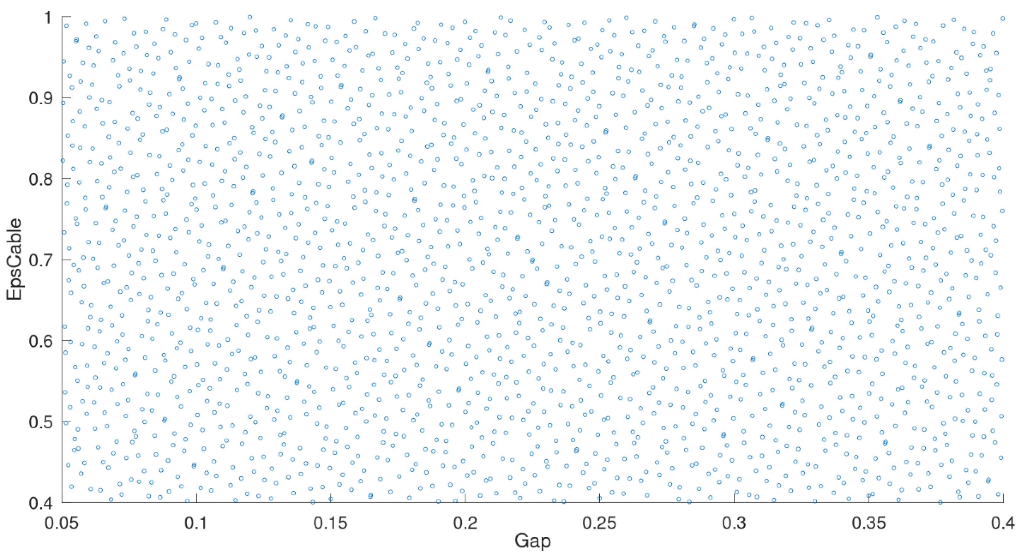
4.3.2. Estimation of Sobol Indices by Monte Carlo Method

First of all, it is important to explain the Monte Carlo method. To keep it simple, it consists of approaching a deterministic value Z as the expectation of the values $z_i$ obtained from a random sample $x_i$ of size N, such as:

$$z_i=f\left(x_i\right) 1\le i\le N$$

(32)

$$\widehat{Z}=\frac{1}{N}{\displaystyle \sum }_{i=1}^N{z}_i$$

(33)

The convergence of $\widehat{Z }$to Z is provided by the strong law of large numbers, which ensures that the larger the sample size N, the closer the Monte Carlo estimate will get to its deterministic value, with a convergence rate of $\mathrm{O}\left(N^{-1/2}\right)$.

Let us now consider a sampling size N such that the p input variable of our model $(X_1,\dots ,X_p)$ is written:

$$X_{\left(N\right)}={\left(x_{k,1},x_{k,2},\dots ,x_{k,p}\right)}_{k=1\dots N}$$

(34)

We can then write the Monte Carlo estimate of the expectation of Y, E[Y], and the variance of Y, V(Y), such as:

$$\widehat{E}\left(Y\right)=\frac{1}{N}{\displaystyle \sum }_{k=1}^{N}f\left(x_{k1},x_{k2},\dots ,x_{kp}\right)$$

(35)

$$\widehat{V}\left(Y\right)=\frac{1}{N}{\displaystyle \sum }_{k=1}^N{f}^2\left(x_{k1},x_{k2},\dots ,x_{kp}\right)-\widehat{E}{\left[Y\right]}^2$$

(36)

The estimation of Sobol sensitivity indices requires the conditional variance expectation estimation. The estimation of first-order sensitivity indices (29) consists of estimating the quantity:

$$V\left(E\left[Y|X_i\right]\right)=E\left[E{\left[Y|X_i\right]}^2\right]-E{\left[E\left[Y|X_i\right]\right]}^2=U_i-E{\left[Y\right]}^2$$

(37)

Sobol proposes to estimate the quantity $U_i$, i.e., the expectation of the square of the expectation of Y conditionally at $X_i$ by varying between the two calls to the function $f$ all the variables except the variable $X_i$. This requires two samples of random realizations of the input variables, noted here $X_{\left(N\right)}^{\left(1\right)}$ and $X_{\left(N\right)}^{\left(2\right)}$. The variance of Y, in (29), is normally calculated as defined in (36).

$${\widehat{U}}_i=\frac{1}{N}{\displaystyle \sum }_{k=1}^{N}f\left(x_{k1}^{\left(1\right)}, \dots ,x_{k\left(i-1\right)}^{\left(1\right)},x_{ki}^{\left(1\right)},x_{k\left(i+1\right)}^{\left(1\right)},\dots ,x_{kp}^{\left(1\right)}\right)x f\left(x_{k1}^{\left(2\right)}, \dots ,x_{k\left(i-1\right)}^{\left(2\right)},x_{ki}^{\left(1\right)},x_{k\left(i+1\right)}^{\left(2\right)},\dots ,x_{kp}^{\left(2\right)}\right)$$

(38)

$$\widehat{E}{\left[Y\right]}^2=\frac{1}{N}{\displaystyle \sum }_{k=1}^{N}f\left(x_{k1}^{\left(1\right)}, \dots ,x_{k\left(i-1\right)}^{\left(1\right)},x_{ki}^{\left(1\right)},x_{k\left(i+1\right)}^{\left(1\right)},\dots ,x_{kp}^{\left(1\right)}\right) x f\left(x_{k1}^{\left(2\right)}, \dots ,x_{k\left(i-1\right)}^{\left(2\right)},x_{ki}^{\left(2\right)},x_{k\left(i+1\right)}^{\left(2\right)},\dots ,x_{kp}^{\left(2\right)}\right)$$

(39)

Concerning the total order Sobol index, we can write the variance of Y according to all parameters except $X_i$, presented in the (31), such as:

$$V\left(E\left[Y|X_{~i}\right]\right)=E\left[E{\left[Y|X_{~i}\right]}^2\right]-E{\left[E\left[Y|X_{~i}\right]\right]}^2=U_{~i}-E{\left[Y\right]}^2$$

(40)

In order to calculate $U_{~i}$, we apply the same method as for $U_i$, but here we vary only the $X_i$ parameter:

$${\widehat{U}}_{~i}=\frac{1}{N}{\displaystyle \sum }_{k=1}^{N}f\left(x_{k1}^{\left(1\right)}, \dots ,x_{k\left(i-1\right)}^{\left(1\right)},x_{ki}^{\left(1\right)},x_{k\left(i+1\right)}^{\left(1\right)},\dots ,x_{kp}^{\left(1\right)}\right)x f\left(x_{k1}^{\left(1\right)}, \dots ,x_{k\left(i-1\right)}^{\left(1\right)},x_{ki}^{\left(2\right)},x_{k\left(i+1\right)}^{\left(1\right)},\dots ,x_{kp}^{\left(1\right)}\right)$$

(41)

Thus, using a Monte Carlo sample size of N, we then need 2N simulations of our model, $f$, to obtain one sensitivity index (first order or total) for a parameter $X_i$, since this estimation requires two sets of randomly obtained samples. Therefore, estimating the first and total order sensitivity indices requires $N\left(2p+1\right)$ calls. In the case of large discrepancies between these two indices, then the indices of higher order than one should be estimated in order to have a more accurate visualization of the sensitivity of the model with respect to the input parameters. Otherwise, the effect of the input variables will be mainly first-order and it will not be useful to look at the intermediate-order indices.

Here, a sample size N of 2000 will be sufficient to estimate the indices for our set of parameters, the model being fast enough to run. However, in order to estimate the confidence interval of these indices, it is illusory to want to use such a sample size in a reasonable time. An estimation by boostrap then seems more suitable.

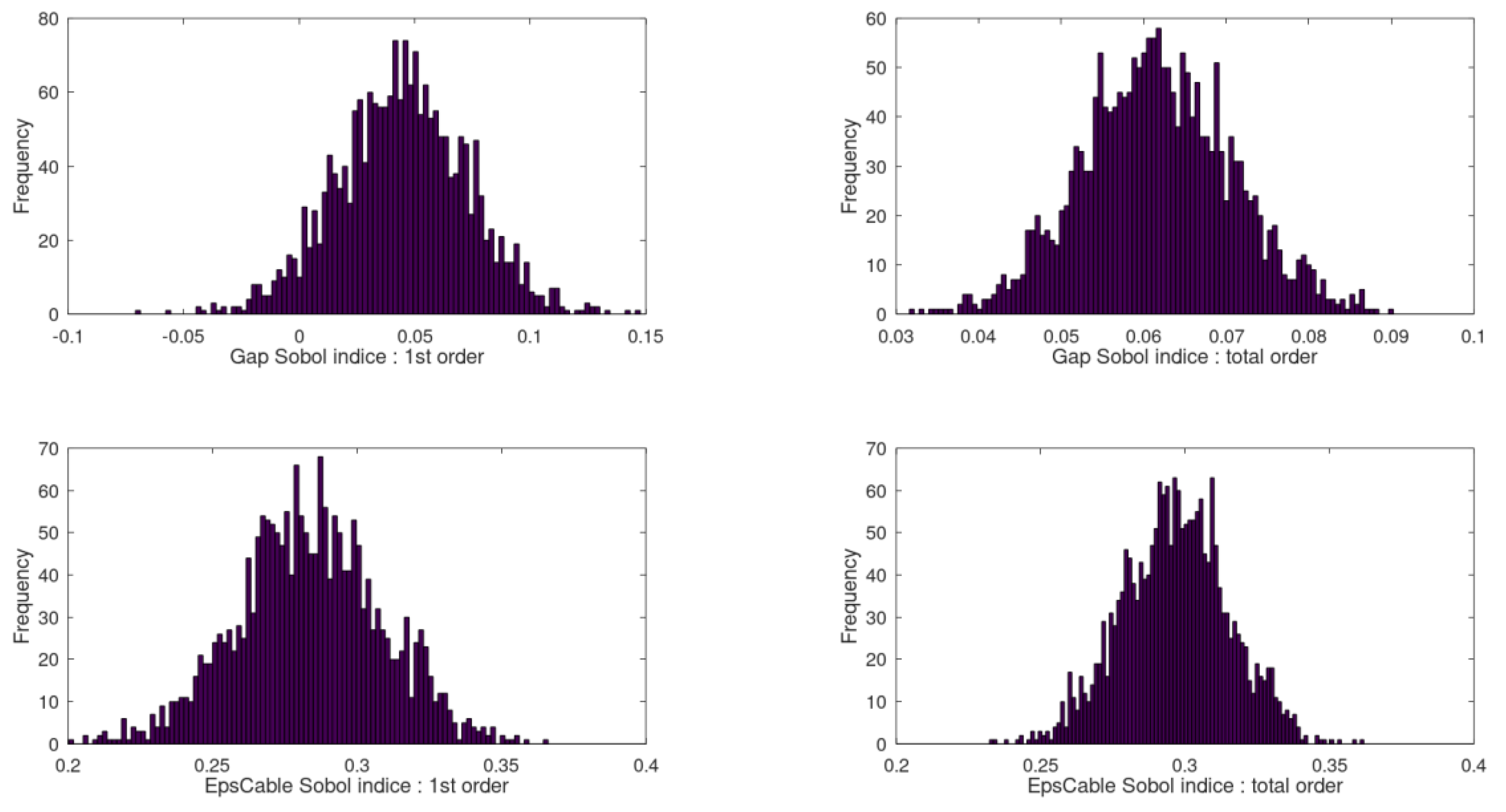
4.3.3. Uncertainty Assessment by Boostrap Method

The boostrap method is a technique to quantify the sensitivity of the output values (standard deviation, confidence interval, mean, etc.) from the original sample, through the statistical analysis of sub-samples.

In order to be more precise, this process is to create random sub-samples from the realizations sample and, for each of the sub-samples, evaluating the desired value, here the Sobol indices. From these sub-samples, we can then derive a statistical analysis such as the variance or the mean, or as far as we are concerned: a confidence interval of 95%.

The application of this method to the model is explained in the next section.

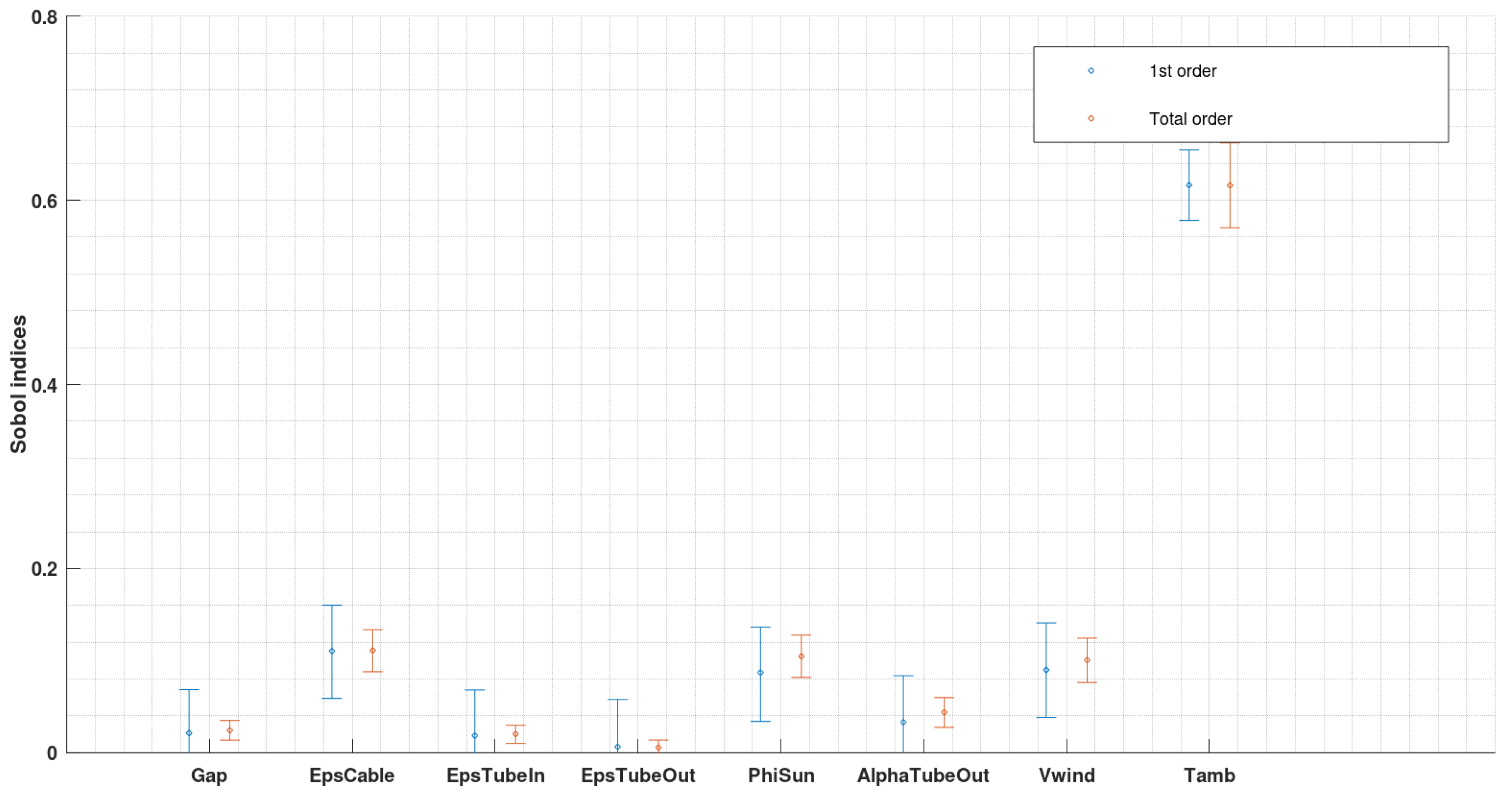
4.3.4. Application

Now that we have defined the elements necessary to calculate the Sobol Indices, we can now apply this methodology to our sensitivity study on the nodal model.

From the intervals of the parameters to be studied, defined in Table 1, we proceed to a random sampling of these parameters, included in their respective interval. We take N = 2000. Nevertheless, it turns out that the precision of value estimates by Monte Carlo method depends on the sampling, as explained previously. With a fixed sample size, we decided to carry out a sampling such that the dispersion of the sample is as uniform as possible, in order to take into account the greatest number of possibilities of input values. This estimation method is then called the quasi Monte Carlo method, based on a low-discrepancy sampling. To do this, we chose a sampling distribution using Sobol sequences. The distinction between these two samples is shown in Figure 5 and Figure 6.

Based on the sampling carried out for each parameter, we performed a statistical analysis using the boostrap method. To do so, we randomly took a subsample of the realizations sample and calculate from it the first-order and total-order Sobol indices, according to (38) and (41). We replicated these calculations for a given number of sub-samples. Here, we chose 2000 sub-samples, each with a size of 1500. We voluntarily choose a large sample size with respect to the initial sample in order to reduce the confidence interval as much as possible. Once all the calculations have been performed, we obtained for each study parameter an estimation of the Sobol indices, as presented in the Figure 7.

From this boostrap method, we calculate for each parameter and each order the mean and the 95% confidence interval. The results are presented in Figure 8 and in

Table 2. Value table of Sobol indices: mean (95% confidence interval: min, max).

	Sobol Indices
	$\mathrm{With}{\theta }_{amb}$		$\mathrm{Without}{\theta }_{amb}$
Parameters	1st order	Total order	1st order	Total order
Gap	0.021 (0, 0.069)	0.024 (0.014, 0.035)	0.045 (0, 0.10)	0.062 (0.044, 0.080)
${\epsilon }_{cable}$	0.11 (0.059, 0.16)	0.11 (0.088, 0.13)	0.28 (0.23, 0.33)	0.30 (0.26, 0.33)
${\epsilon }_{Tub{e}_{In}}$	0.019 (0, 0.068)	0.020 (0.010, 0.030)	0.034 (0, 0.089)	0.050 (0.034, 0.065)
${\epsilon }_{Tub{e}_{Out} }$	0.006 (0, 0.058)	0.006 (0, 0.014)	0.003 (0, 0.057)	0.014 (0, 0.030)
${\varphi }_{sun}$	0.087 (0.034, 0.14)	0.10 (0.082, 0.13)	0.22 (0.16, 0.27)	0.27 (0.23, 0.32)
${\alpha }_{tub{e}_{out}}$	0.033 (0, 0.083)	0.044 (0.028, 0.060)	0.074 (0.020, 0.12)	0.11 (0.084, 0.14)
$V_{wind}$	0.090 (0.038, 0.14)	0.10 (0.076., 0.12)	0.22 (0.17, 0.27)	0.27 (0.22, 0.30)
${\theta }_{amb}$	0.62 (0.58, 0.65)	0.62 (0.57, 0.66)	/	/

.

Firstly, the small difference between first-order indices and total orders indicates that parameter interaction phenomena have little influence on the sensitivity of the model. Consequently, it will not be necessary to calculate intermediate-order indices afterwards.

Secondly, we can observe the dominance of the influence of outside temperature ${\theta }_{amb}$ on the cable temperature. On the other hand, its large value leads to a decrease in the other Sobol indices, explained by the decomposition of the variance (30). In order to study in more detail the influence of the other parameters on the cable temperature, we calculated the Sobol indices with the exception of ${\theta }_{amb}$, presented in Figure 9 and Table 2.

5. Discussion

From these new results, we can observe that meteorological phenomena such as the Sun, the wind and the ambient temperature have a major influence on the thermal behavior of the cable within the J-tube. A continuous measurement of their values would therefore be essential in order to correctly control the heating of the cable, and consequently its ampacity.

One notes that the emissivity of the cable ${\epsilon }_{cable}$, has a significant influence on its heating. We saw in Figure 4 that increasing ${\epsilon }_{cable}$ leads to weak improvements. Nevertheless, with the calculation of the Sobol index, we can affirm that an accurate assessment of its emissivity is highly recommended. Indeed, this value of 0.9, used in [3,4,5,7,8], can be questioned. A more rigorous estimation would allow for a more accurate evaluation of the temperature of the cable conductor, used in the calculation of the ampacity. In contrast, we observe that the influence of the tube’s surface emissivity ${\epsilon }_{tub{e}_{in}},{\epsilon }_{tub{e}_{out}}$ is relatively low. Thus, we can say that the choice of the type of J-tube (plastic or iron) is not significant, in order to increase the current ampacity of the cable. However, a better definition of these values could slightly improve the numerical model.

The solar absorptivity of the outside surface $\alpha$ is relatively influential, but unlike the latter, optimization of this parameter could greatly improve the cable's ampacity. Similarly, accurate characterization is necessary in order to build a viable numerical model for industrial uses.

Finally, we can observe that the gap between the cable and the tube has a relatively low influence on core temperature. Here, the gap and the exchange coefficient inside the tube $h_{conv}$ are strongly linked: increasing the distance between the cable and the tube will allow more air circulation which would result in a reduction of the cable temperature. However, it is clear here that increasing the gap will not lead to more noticeable convection, due to the correlation (7). Nevertheless, this correlation should be questioned, natural convection between concentric cylinders with a high aspect ratio being more complex than a correlation (turbulence, temperature stratification).

6. Conclusions

In this article, we present a numerical model in order to rate the temperature of a cable installed inside a J-tube, not considered in IEC 60287, based on the lumped element method. This one is then compared to previous work for validation, with relative success. Furthermore, contrarily to the previous one, this model is more flexible, giving access to a 2D temperature field in a more physical way. It is even possible to access transient calculations by adding thermal capacities to each node. This work is still in progress.

With a valid model, a sensibility analysis based on local and global analysis is presented in this paper. We found that weather is the most impactful parameter on cable current ampacity (sun, wind, ambient temperature) and should be controlled continuously in order to manage overheating. Otherwise, we found that cable surface emissivity should be better assessed because of its strong influence on the cable temperature, in contrast to J-tube surfaces. Finally, even if thermal exchanges between the cable and the tube are dominated by radiation in this case, an improvement of the inner convection should lead to concrete optimisation of the cable current ampacity. However, this last statement should be verified with further studies.

References

- IEC. Electric Cables—Calculation of the Current Rating—Part 1-1: Current Rating Equations (100% Load Factor) and Calculation of Losses—General; IEC: Geneva, Switzerland, 2014. [Google Scholar]
- IEC. Electric Cables—Calculation of the Current Rating—Part 2-1: Thermal Resistance—Calculation of Thermal Resistance; IEC: Geneva, Switzerland, 2015. [Google Scholar]
- Coates, M.; Coates, M. Rating Cables in J-Tube; Report No. 88-0108; ERA technology: Leatherland, UK, 1988. [Google Scholar]
- Hartlein, R.A.; Black, W.Z. Ampacity of electric power cables in vertical protective risers. IEEE Trans. Power Appar. Syst. 1983, PAS-102, 1678–1686. [Google Scholar] [CrossRef]
- Anders, G.J. Rating of cables on riser poles. In Jicable; Paris-Versailles: Paris, France, 1995; pp. 602–607. [Google Scholar]
- Anders, G.J. Rating of cables on riser poles, in trays, in tunnels and shafts. IEEE Trans. Power Deliv. 1996, 11, 3–11. [Google Scholar] [CrossRef]
- Chippendale, R.; Cangy, P.; Pilgrim, J. Thermal Rating of J tubes using Finite Element Analysis Techniques. Jicable 2015, 2015, 4–9. [Google Scholar]
- Chippendale, R.D.; Pilgrim, J.A.; Goddard, K.F.; Cangy, P. Analytical thermal rating method for cables installed in J-Tubes. IEEE Trans. Power Deliv. 2017, 32, 1721–1729. [Google Scholar] [CrossRef]
- You, L.; Wang, J.; Liu, G.; Ma, H.; Zheng, M. Thermal Rating of Offshore Wind Farm Cables Installed in Ventilated J-Tubes. Energies 2018, 11, 545. [Google Scholar] [CrossRef]
- Arancio, J.A.; Ould El Moctar, M.; Nguyen-tuan, M.; Roques, J.P.; Tayat, F. Thermal rating of submarine cables installed in J-tube using Lumped Element Method. In Proceedings of the Jicable19, Paris-Versailles, France, 23–27 June 2019; pp. 2–6. [Google Scholar]
- CIGRE. Calcul de la température des câbles dans les tunnels ventilés. Electra 1992, 143, 38–59.
- Pilgrim, J.A.; Swaffield, D.J.; Lewin, P.L.; Larsen, S.T.; Waite, F.; Payne, D. Rating independent cable circuits in forced-ventilated cable tunnels. IEEE Trans. Power Deliv. 2010, 25, 2046–2053. [Google Scholar] [CrossRef]
- Hamby, D.M. A Review of Techniques for Parameter Sensitivity. Environ. Monit. Assess. 1994, 32, 135–154. [Google Scholar] [CrossRef] [PubMed]
- Sobol, I.M. Global sensitivity indices for nonlinear mathematical models and their Monte Carlo estimates. Math. Comput. Simul. 2001, 55, 271–280. [Google Scholar] [CrossRef]
- Jacques, J. Pratique de l’analyse de sensibilité : Comment évaluer l’impact des entrées aléatoires sur la sortie d’un modèle mathématique. Lille sn 2011, 71, 266–276. [Google Scholar]
- Iooss, B. Review of global sensitivity analysis of numerical models. J. De La Société Française De Stat. 2011, 151, 3–25. [Google Scholar]
- Dorison, E.; Protat, F. Current rating of cables installed in tunnels. Jicable 2007, 2007, 19–23. [Google Scholar]
- Keyhani, M.; Kulacki, F.A.; Christensen, R.N. Free Convection in a Vertical Annulus with Constant Heat Flux on the Inner Wall. J. Heat Transf. 1983, 105, 454–459. [Google Scholar] [CrossRef]
- Saltelli, A.; Homma, T. Importance measures in global sensitivity analysis of model output. Reliab. Eng. Syst. Saf. 1996, 52, 1–17. [Google Scholar]