A Feasibility Study of Machine Learning Based Coarse Alignment ^†

Abstract

Inertial navigation systems (INSs) require an initial attitude before its operation. To that end, the coarse alignment process is applied using inertial sensors readings. For low-cost inertial sensors, only the accelerometers readings are processed to yield the initial roll and pitch angles. The accuracy of the coarse alignment procedure is vitally important for the navigation solution accuracy due to the navigation solution drift accumulating over time. In this paper, we propose using machine learning (ML) approaches, instead of traditional approaches, to conduct the coarse alignment procedure. To that end, a new methodology for the alignment process is proposed, based on state-of-the-art ML algorithms such as random forest (RF) and the more advanced boosting method of gradient tree XGBoost. Results from a simulated alignment of stationary INS scenarios are presented accompanied by a feasibility study. ML results are compared with the traditional coarse alignment methods in terms of time to convergence and accuracy performance. When using the proposed approach, with the examined scenarios, results show a significant improvement of the accuracy and time required for the alignment process.

1. Introduction

An inertial navigation system (INS) is a dead reckoning (DR) navigation system that integrates the inertial sensors outputs to give the current position, velocity, and attitude of a platform without any external aids [1,2]. As required from a DR system, it must have the state initial conditions before initiating the navigation solution. INS inertial sensors contain an accelerometer triad (three mutually orthogonal accelerometers) that measure the specific force vector, and a gyroscope triad aligned with the accelerometers that measure the angular rate vector [2]. Present INS systems are commonly based on micro-electro-mechanical-system (MEMS) technology that applies small and cheap sensors but with relatively high errors that can dramatically affect the overall navigation solution performance [3,4,5].

The initialization of the position and velocity vectors is made using external information (such as from global navigation satellite systems). The initial attitude, however, can be determined using inertial sensors [5,6,7]. This process starts with an essential step of coarse alignment (CA) whose purpose is to calculate the initial attitude angles—roll and pitch from the accelerometer’s readings and yaw from the gyroscope’s readings. For low-cost inertial sensors only, the roll and pitch can be determined from the accelerometers [2,8]. When completing the CA procedure, fine alignment (FA) is applied to improve the CA results. To that end, FA uses external sensors or information, such as zero velocity updates, in a fusion process to improve the accuracy [2,6]. Recently, an analytic evaluation of the steady-state properties of the FA process was derived [9].

In this paper, we address the CA problem for low-cost sensors. We aim to demonstrate the ability to predict the initial roll and pitch angles, using computational learning algorithms, given its inertial sensors readings and a priori database containing the system behavior from other previously recorded alignment scenarios. In the prediction solution, we show improvement of the accuracy and time required for the alignment process, which makes it possible using learning algorithms to replace the classical coarse alignment with a computational learning alignment method. The development of this new ability to perform the process of aligning the INS quickly and accurately by smart integration of machine learning (ML) algorithms can constitute a breakthrough in autonomous vehicle navigation in an environment that does not allow the significant use of additional means of updating the navigation system.

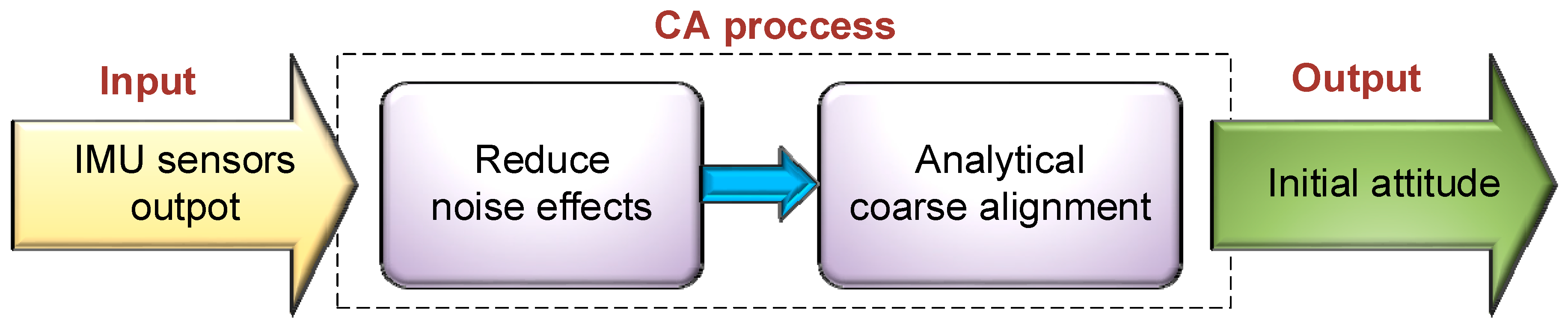
2. Traditional Coarse Alignment

The traditional CA process of an inertial navigation system is illustrated in Figure 1. It consists of two main steps: The first step is some pre-processing of the input sensors readings whose purpose is to reduce the random noise effects. Next, the initial values of the roll and pitch attitudes are calculated using an analytical transformation of the values to the current attitude of the system [1].

Once we reduced the influence of the random noise effects correctly, the performance of the inertial measurement unit (IMU) sensors limits the accuracy of the initial attitude [6]. The method to address these noise effects is to take the accelerometer measurements over time and average them. This method is significantly time-consuming and directly affects the overall performance of the alignment process.

The analytical calculation is based on the following coordinate transformation matrix, in terms of the pitch θ and roll ϕ Euler angles of the INS [2]:

$$f=\left[\begin{array}{c}\sin \theta \\ -\cos \theta \sin \varphi \\ -\cos \theta \cos \varphi \end{array}\right]g$$

(1)

where g is the gravity magnitude and $f$ is the specific force vector expressed in the INS body frame given by:

$$f=\left[\begin{array}{c}{f}_x\\ f_y\\ f_z\end{array}\right]$$

(2)

The pitch and roll may be determined analytically by using the following equations of the reverse transformation [2]:

$$\theta =arctg\left(\frac{-f_x}{\sqrt{f_y{}^2+f_z{}^2}}\right)$$

(3)

$$\varphi =arctg2(-f_y,-f_z)$$

(4)

In practice, the values of the force vector $f$ in Equations (3) and (4) are calculated by taking the mean values of the accelerometer measurements for a given period.

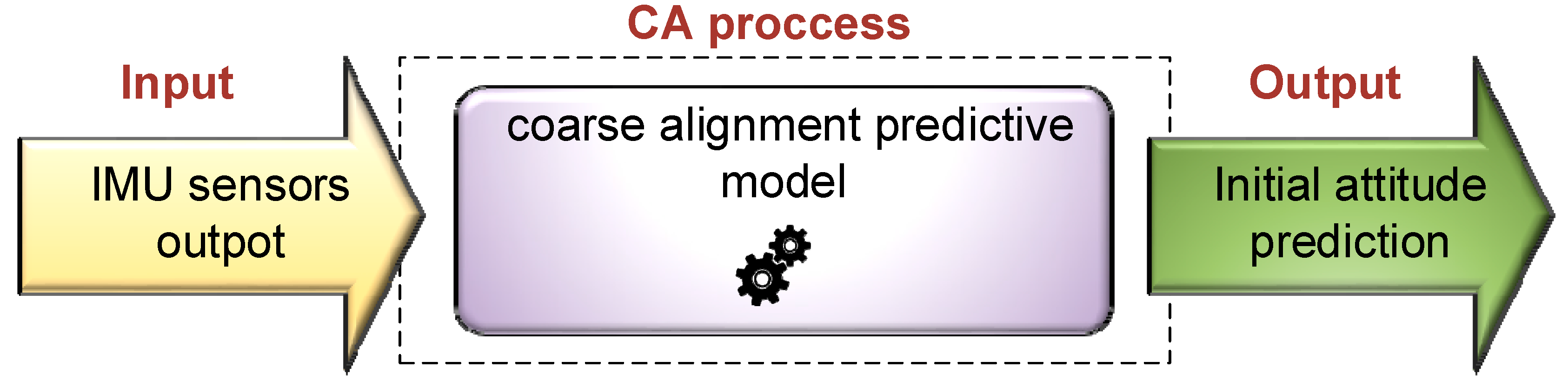
3. Machine Learning Methodology

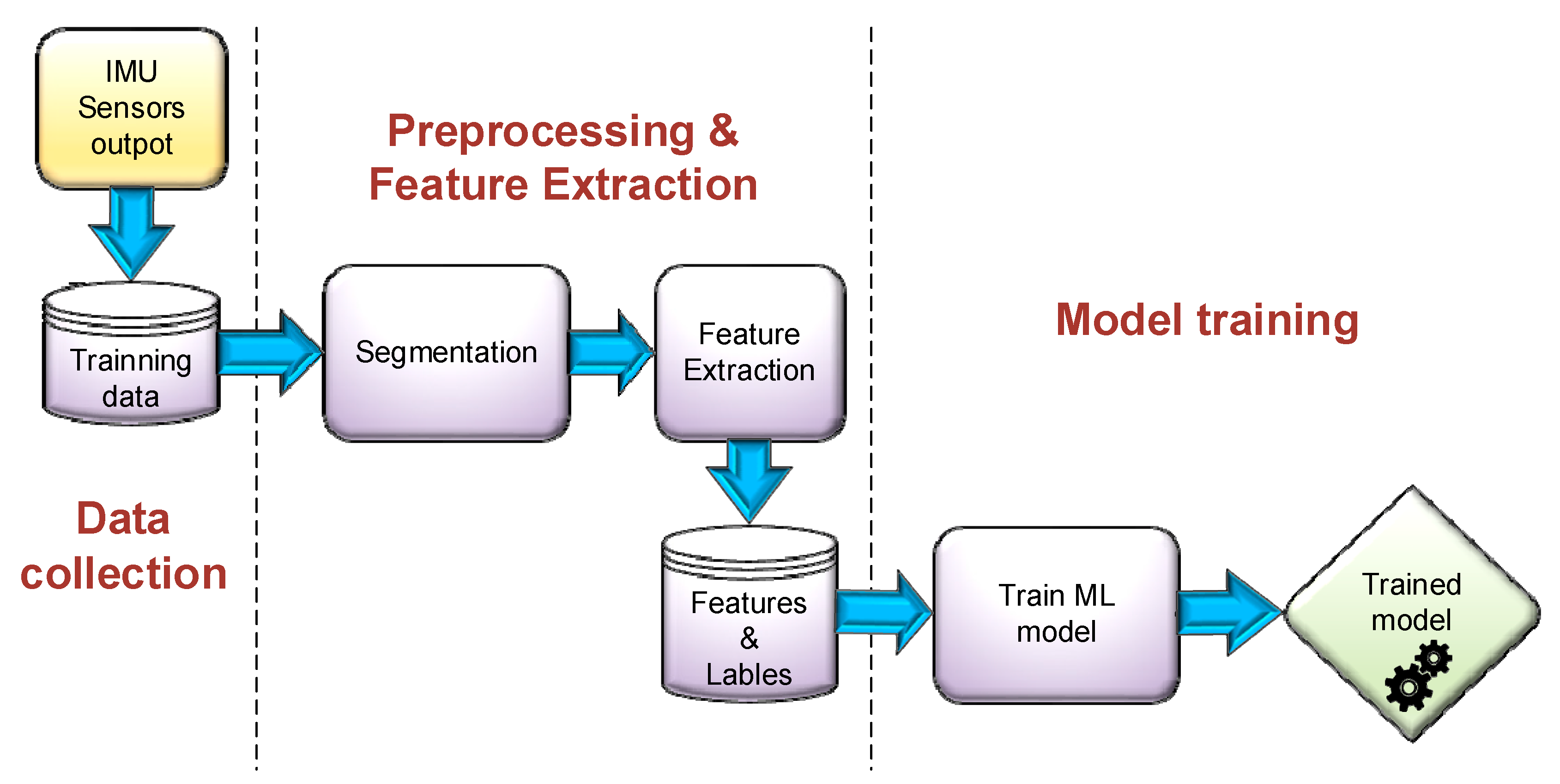
3.1. Overall Approach

The basic idea is to replace the traditional process with a new one based on a pre-learned CA predictive ML model, as being illustrated in Figure 2. The new process will predict the initial attitude state given IMU sensors readings of a relatively short period. The CA task is treated as a supervised, regression machine learning problem. We have both the feature’s—the data of the accelerometer measurements, and the target labels—continuous values of true pitch and roll that we want to predict.

The idea is to train and evaluate the performance of multiple machine learning models in terms of both prediction speed and accuracy on a pre-recorded large time series dataset of accelerometers readings and the matching true-attitudes. For the feasibility study, the data were obtained from simulations of the inertial sensors in a stationary system, having a velocity random walk error. Then, we evaluated the results in terms of absolute errors prediction, and our goal was to show that the new process can perform better than the traditional method. Having better (or the same) accuracy within a shorter time, or overall better accuracy in similar time (or even longer one) will constitute an interesting, innovative result.

Figure 3 illustrates the process in which our predictive model was trained. First, we generated and stored time-series data for each running scenario. The input data consist of the raw accelerometers readings values ${\mathrm{X}}_t={\text{{}\mathrm{x}}_1,\mathrm{\dots }{,\mathrm{x}}_{\mathrm{n}}\text{}}$ of three accelerometer axes ${\text{{}\mathrm{a}}_x{,\mathrm{a}}_y{,\mathrm{a}}_z\text{}}$ and the matching target labels of true pitch and true roll ${\mathrm{Y}}_t={\text{{}\mathrm{y}}_1,\mathrm{\dots }{,\mathrm{y}}_{\mathrm{n}}\text{}}$. Given the time-series data, it is critical to identify some strong features for the success of the trained model in the prediction task. To calculate features from the raw data, the next step was to do some pre-processing work on the given time series, in which we used sliding window method to split the whole data set into segments. Each data segment has a fixed width of w samples. Then, for each data segment, numerical features extraction (FE) was applied for usage in the final stage of the modeling process.

The selection of the segment width w has a high significance, as it determines the actual amount of accelerometer raw data that needed to accumulate before we can predict the roll and pitch. Using a smaller width means a faster alignment process, which requires less time to converge, but can influence the accuracy performance. To determine the optimal duration value, we tested a range of segment widths for each of the ML methods and compared the results with the traditional alignment method.

We define the inertial sensors error model to express the influence of the random noise (white noise) component while analyzing the CA performance [8]. The specific force vector sensed by the accelerometers has the following form [2]:

$${\tilde{f}}_{imu}=f_{true}+b_a+{\mathrm{w}}_a$$

(5)

where $f_{true}$ is the real true value of the specific force, $b_a$ is the accelerometers biases, and ${\mathrm{w}}_a$ is the inertial sensors random noise.

3.2. Features Description

Our dataset includes a total of 16 known continuous numerical features that were computed on the signals of the accelerometer’s axes, within each time segment. The features can be general categories as follows:

• Basic statistical features: Mean, Standard deviation, Variance, Minimum value, Absolute of the minimum value, Maximum value, Absolute of the maximum value.
• Advanced statistical features:
  • Entropy: the amount of regularity and the unpredictability.
  • Skewness: the asymmetry of the probability distribution.
  • Kurtosis: the “tailedness” of the probability distribution.
  • Energy: the sum of squares of values.
  • Amplitude: the difference between the minimum and the maximum value.
• Time-Domain Features:
  • Number of peaks: the number of peaks with defined minimum peak height and the minimum distance between peaks.
  • Mean spectral energy: the mean spectral energy computation using one-dimensional discrete Fourier Transform.
  • Mean crossing rate: the number of mean crossings.
  • Zero-crossing rate: the number of sign changes.

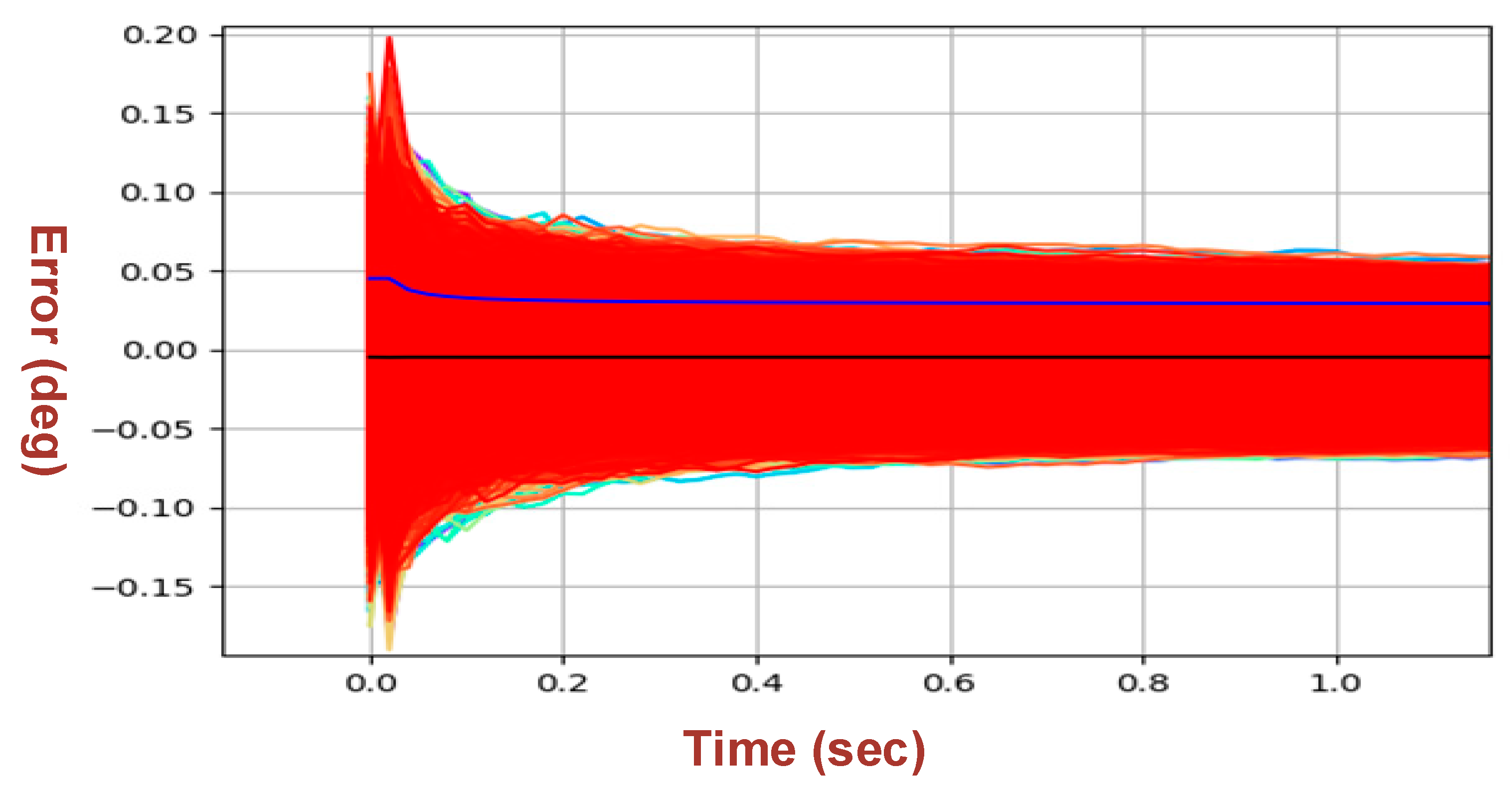
4. Results and Discussion

Accelerometers readings of a low to mid accuracy with a velocity random walk (VRW) error [10] of 0.03 to 0.05 $m/s/\sqrt{h}$, respectively, in stationary conditions were simulated for the feasibility study. The other accelerometer error terms, such as bias, were not addressed in the feasibility study. The simulated raw data generated for selected sets of true pitch and true roll angles of the accelerometers. Two representative sets differing by their resolution were chosen for the analysis: First, within a small range of angles −1° ≤ roll, pitch ≤ 1° with a relatively high resolution of 0.01 degrees and then a wider range of −180 < roll < 180 and −90 < pitch < 90 in smaller resolution. The motivation for this strategy was to deal with the huge amount of information collected from the simulative accelerometers which are operating in 50Hz, and still try to examine the ability of machine learning based CA both in a wide angles range and also to distinguish between in high resolution of accuracy.

For performance comparison between the traditional CA to the ML CA, the mean absolute error (MAE) measure was employed to evaluate the alignment precision and convergence time. The initial ML CA was RF [11] and then the gradient tree XGBoost [12], a more advanced boosting method, was examined.

The result shows that in the challenging case of low accuracy IMU with a high-resolution test set while using the traditional CA method the converges to an MAE of about 0.005 (±0.029) degrees, after about 2 s, and maintains this value even after few more seconds. Figure 4 shows, for example, the actual results of all the test set runs roll errors spread, with the mean value and standard deviation (STD) marked on top, in black and blue lines respectively. Figure 5 shows the mean and STD of those results separately.

Table 1. Roll attitude errors statistical analysis.

Parameters	Classical Method	RF
Convergence time	2 s	1 s
MAE (deg)	0.005 (±0.029)	0.0039 (±0.0031)

present the results comparison for the same scenario of low accuracy IMU with a high-resolution test set, between classical CA and ML-based CA in the best configuration of each of the methods, including the convergence time and the precision in terms MAE. Both ML methods performed better relative to classical CA, and the best setup was one with RF obtaining an MAE of 0.0039 (±0.0031) after one second. That is an accuracy improvement both in the mean and STD error values of 0.0011 and 0.0259 degrees respectively. After RF, The XGBoost also showed good accuracy improvement over the classical CA of 0.009 and 0.0257 degrees for the mean and STD error values respectively. Both the ML methods convergence to those results after only 1 s that is half the convergence time of the classic process. That is, performance was improved both in time to convergence and accuracy of the CA process.

5. Conclusions

The goal of this work was to show the feasibility of implementing machine learning based coarse alignment process instead of the traditional approaches, with an added value of improvement in accuracy and/or time required for the alignment process. The results show a significant improvement in these parameters in a simulative environment. This improvement is an important breakthrough in the area of coarse alignment of inertial navigation and in particular in autonomous vehicle navigation. In future work, we aim to continue and expand the research on the proposed approach in several main aspects including implementation of neural networks and conducting field experiments to validate the proposed approach.

References

1. Titterton, D.H.; Weston, J.L. Strapdown Inertial Navigation Technology, 2nd ed.; The American Institute of Aeronautics and Astronautics and the Institution of Electrical Engineers: Reston, VA, USA, 2004. [Google Scholar]
2. Groves, P.D. Principles of GNSS, Inertial and Multisensor Integrated Navigation Systems, 2nd ed.; Artech House: Norwood, MA, USA, 2013. [Google Scholar]
3. Aggarwal, P.; Syed, Z.; Noureldin, A.; El-Sheimy, N. MEMS-Based Integrated Navigation; ARTECH HOUSE: Boston, London, 2010. [Google Scholar]
4. Baird, W.H. An introduction to inertial navigation. Am. J. Phys. 2009, 77, 844–847. [Google Scholar] [CrossRef]
5. Bistrov, V. Performance Analysis of Alignment Process of MEMS IMU. Int. J. Navig. Obs. 2012, 2012, 1–11. [Google Scholar] [CrossRef]
6. Hailiang, W.; Guozhang, L.; Zhiyong, S. Overview of Initial Alignment Method for Strap down Inertial Navigation System. In Proceedings of the, Tianjin, China, 10–11 June 2017; Volume 114, pp. 149–154. [Google Scholar]
7. Han, S.; Wang, J. A Novel Initial Alignment Scheme for Low-Cost INS Aided by GPS for Land Vehicle Applications. J. Navig. 2010, 63, 663–680. [Google Scholar] [CrossRef]
8. Vaknin, E.; Klein, I. Coarse leveling of gyro-free INS. Gyroscopy Navig. 2016, 7, 145–151. [Google Scholar] [CrossRef]
9. Tsukerman, A.; Klein, I. Analytic Evaluation of Fine Alignment for Velocity Aided INS. IEEE Trans. Aerosp. Electron. Syst. 2018, 54, 376–384. [Google Scholar] [CrossRef]
10. Woodman, O.J. An Introduction to Inertial Navigation; Technical Report; University of Cambridge: Cambridge, UK, 2007. [Google Scholar]
11. Breiman, L. Machine Learning; Kluwer Academic Publishers: Dordrecht, The Netherlands, 2001. [Google Scholar] [CrossRef]
12. Tianqi, C.; Carlos, G. XGBoost: A Scalable Tree Boosting System. In Proceedings of the 22nd ACM SIGKDD International Conference on Knowledge Discovery and Data Mining (KDD ‘16), San Francisco, CA, USA, 13–17 August 2016; ACM: New York, NY, USA, 2016; pp. 785–794. [Google Scholar] [CrossRef]
Figure 1. Traditional inertial navigation system coarse alignment (CA) process.
Proceedings 04 00050 g001
Figure 2. Proposed CA process.
Proceedings 04 00050 g002
Figure 3. CA predictive model training process.
Proceedings 04 00050 g003
Figure 4. Attitude errors of the traditional coarse alignment.
Proceedings 04 00050 g004
Figure 5. Mean and STD errors of the traditional coarse alignment.
Proceedings 04 00050 g005