Using Entropy to Forecast Bitcoin’s Daily Conditional Value at Risk ^†

Abstract

Conditional value at risk (CVaR), or expected shortfall, is a risk measure for investments according to Rockafellar and Uryasev. Yamai and Yoshiba define CVaR as the conditional expectation of loss given that the loss is beyond the value at risk (VaR) level. The VaR is a risk measure that represents how much an investment might lose during usual market conditions with a given probability in a time interval. In particular, Rockafellar and Uryasev show that CVaR is superior to VaR in applications related to investment portfolio optimization. On the other hand, the Shannon entropy has been used as an uncertainty measure in investments and, in particular, to forecast the Bitcoin’s daily VaR. In this paper, we estimate the entropy of intraday distribution of Bitcoin’s logreturns through the symbolic time series analysis (STSA) and we forecast Bitcoin’s daily CVaR using the estimated entropy. We find that the entropy is positively correlated to the likelihood of extreme values of Bitcoin’s daily logreturns using a logistic regression model based on CVaR and the use of entropy to forecast the Bitcoin’s daily CVaR of the next day performs better than the naive use of the historical CVaR.

1. Introduction

In finance, risk management is the activity of identifying, analyzing, estimating and controlling the risk of losing money. For our purposes, risk management is a procedure for shaping a loss distribution of an investment. The value at risk (VaR) is the most popular risk measure and it represents how much an investment might lose during usual market conditions with a given probability in a time interval. In other words, VaR is a percentile of a loss distribution. Another very popular risk measure is the conditional value at risk (CVaR), or the expected shortfall. CVaR is a risk measure for investments reintroduced in the literature by Rockafellar and Uryasev [1], for a former reference see Love et al. [2]. According to Sarykalin et al. [3], it approximately (or exactly, under certain conditions) equals the average of some percentage of the worst-case loss scenarios.

Relative to the definitions, there is a near correspondence between VaR and CVaR. For instance, Yamai and Yoshiba [4] defined CVaR as the conditional expectation of loss given that the loss is beyond the VaR level. Consequently, considering the same confidence level, VaR is a lower bound for CVaR. In particular, Rockafellar and Uryasev [1,5] showed that CVaR is superior to VaR in applications related to investment portfolio optimization. In practice, the choice between VaR and CVaR rests on the differences in mathematical properties, stability of statistical estimation, simplicity of optimization procedures, acceptance by regulators, and so on [3]. For instance, in terms of mathematical properties, the CVaR of a portfolio is a continuous and convex function with respect to positions in instruments, whereas the VaR may be even a discontinuous function.

The volatility is the standard deviation of the distribution of logreturns and a very simple and earlier measure of financial risk. The corresponding variance is a natural measure of the statistical uncertainty but it just captures a small portion of the informational content of the distribution of the logreturns. On the other hand, the entropy is a more general measure of uncertainty than the variance because it may be related to higher-order moments of a distribution [6,7,8]. According to Dionisio et al. [8], the variance measures the concentration around the mean while the entropy measures the dispersion of the density irrespective of the location of the concentration. Finally, for Pele et al. [9], the entropy of a distribution function is strongly related to its tails and this feature is more important for distributions with heavy tails or with an infinite second-order moment for which the variance does not make sense.

In the literature, there are empirical papers showing that entropy has good predictive power for risk. For instance, Billio et al. [10] showed that entropy has the ability to forecast and predict banking crises using directly the entropy of systemic risk measures. In addition, Pele et al. [9] showed that entropy of the intraday distribution of logreturns is a strong predictor of daily VaR, performing better than the classical GARCH models, for a time series of EUR/JPY exchange rates. Similarly, Pele and Mazurencu-Marinescu-Pele [11], instead of using the entropy of the intraday distribution of logreturns, defined the entropy using symbolic time series analysis (STSA) showing that their entropy is a strong predictor of daily VaR, performing better than the classical GARCH models, using high-frequency data for Bitcoin.

There is a recent interest in the statistical properties and risk behavior of cryptocurrencies [12,13,14] and, in particular, Bitcoin [15]. Consequently, in this paper, we estimate the entropy of the symbolic intraday distribution of Bitcoin’s logreturns through the STSA [11] and we model and forecast the Bitcoin’s daily CVaR using the estimated entropy. The main contribution of this paper is the extension of the study performed by Pele and Mazurencu-Marinescu-Pele [11] to include the CVaR. The rest of the paper is organized as follows: in Section 2, we present the details of the methodology; in Section 3, we present our empirical study describing the dataset, the results and the corresponding comments; finally, in Section 4, we conclude the paper.

2. Methodology

In this section, we review the methodology to estimate the entropy of the symbolic intraday distribution of logreturns through the STSA, a logistic model connecting the daily VaR and the entropy, and a forecasting model for the daily VaR using the entropy based on a quantile regression published by Pele and Mazurencu-Marinescu-Pele [11]. In addition, we introduce the two main contributions of this paper: a logistic model connecting the daily CVaR and the entropy, and a forecasting model for the daily CVaR using the entropy based on a modified quantile regression model. It is also important to mention that the Bitcoin exchange rate is hereinafter referred to as Bitcoin price.

2.1. Entropy of Symbolic Intraday Logreturns

In the intraday context, it is usual to consider a set of days $d\in \left\{1,\cdots ,D\right\}$ and each day equally partitioned in M time bins. Consequently, for a day d and a time bin $m\in \left\{1,\cdots ,M\right\}$, we associate a price $P_{d,m}$ and a logprice $p_{d,m}=ln{P}_{d,m}$. Then, the intraday logreturn of an asset is defined as follows:

$$r_{d,m}=p_{d,m}-p_{d,m-1};d=1,\cdots ,D;m=2,\cdots M.$$

(1)

For the empirical study of this paper, it is possible to define $r_{d,1}=p_{d,1}-p_{d-1,M};d=2,\cdots ,D$ because the Bitcoin is continuously traded. However, it is important to point that for other kind of assets, it would be better to ignore the logreturn $r_{d,1}$. In addition, $r_{1,1}$ is not defined.

The intraday logreturns is usually very noisy. The idea behind the STSA technique [16] to produce low-resolution data from high-resolution data. In particular, STSA is a transformation of a real number sequence to a binary sequence. In our case, the STSA transformation is applied to the intraday logreturn to obtain the symbolic intraday logreturn. The symbolic intraday logreturn is defined as follows:

$$s_{d,m}=\left\{\begin{array}{cc}1,& r_{d,m}\le 0\\ 0,& r_{d,m}>0\end{array}\right..$$

(2)

Basically, the symbolic intraday logreturn is a binary sequence of 0s representing increasing prices and 1s representing decreasing prices.

Based on the Shannon entropy definition [17], the entropy of the symbolic intraday logreturns is defined as follows:

$$h_d=-{\pi }_d{log}_2{\pi }_d-\left(1-{\pi }_d\right){log}_2\left(1-{\pi }_d\right),$$

(3)

where ${\pi }_d=Pr\left(s_{d,m}=1\right)$ and $1-{\pi }_d=Pr\left(s_{d,m}=0\right)$. It is possible to notice that the entropy of the symbolic intraday logreturns is a daily entropy. In addition, we estimate ${\pi }_d,d=2,\cdots ,D$ using the sample frequency ${\sum }_{m=1}^M{s}_{d,m}/M,d=2,\cdots ,D$ and ${\pi }_1$ using the sample frequency ${\sum }_{m=2}^M{s}_{1,m}/\left(M-1\right)$.

2.2. Entropy and Daily VaR and CVaR

Intuitively, the entropy of the symbolic intraday logreturns is higher at the presence of higher uncertainty in the returns and lower at the presence of lower uncertainty in the returns. Consequently, the likelihood of extreme negative daily logreturns is explained by higher values of entropy. In [11], it was verified that the entropy is positively correlated to the likelihood of extreme negative daily logreturns and the relation between VaR and entropy was modeled using the following logistic regression model:

$$Pr\left(y_d=1\right)=\frac{e^{b_0+b_1{h}_d}}{1+e^{b_0+b_1{h}_d}},$$

(4)

where $b_0$ and $b_1$ are constants to be estimated;

$$y_d=\left\{\begin{array}{cc}1,& r_d\le -{\mathrm{VaR}}_{\alpha }\\ 0,& r_d>-{\mathrm{VaR}}_{\alpha }\end{array}\right.,d=2,\cdots ,D$$

(5)

are the indicators of the lower tails of the daily logreturns; $r_d=ln{P}_d-ln{P}_{d-1},d=2,\cdots ,D$ are the daily logreturns; $P_d$ is the closing price of day d; and ${\mathrm{VaR}}_{\alpha }$ is the daily value at risk at the significance level $\alpha \in \left]0,1\right[$ defined by

$$Pr\left(r_d\le -{\mathrm{VaR}}_{\alpha }\right)=\alpha$$

(6)

or, alternatively,

$${\mathrm{VaR}}_{\alpha }=-inf\left\{z\left|F\right(z)\ge \alpha \right\},$$

(7)

where $F\left(·\right)$ is the cumulative distribution function of the daily logreturns.

In this paper, the hypothesis is also that the entropy is positively correlated to the likelihood of extreme negative daily logreturns and we model the relation between CVaR and entropy using the following logistic regression model:

$$Pr\left(u_d=1\right)=\frac{e^{c_0+c_1{h}_d}}{1+e^{c_0+c_1{h}_d}},$$

(8)

where $c_0$ and $c_1$ are constants to be estimated;

$$u_d=\left\{\begin{array}{cc}1,& r_d\le -{\mathrm{CVaR}}_{\alpha }\\ 0,& r_d>-{\mathrm{CVaR}}_{\alpha }\end{array}\right.,d=2,\cdots ,D$$

(9)

are the indicators of the lower tails of the daily logreturns; and ${\mathrm{CVaR}}_{\alpha }$ is the daily conditional value at risk at the significance level $\alpha \in \left]0,1\right[$ defined by

$${\mathrm{CVaR}}_{\alpha }=-\frac{1}{\alpha }{\int }_{-\infty }^{-{\mathrm{VaR}}_{\alpha }}zf\left(z\right)dz,$$

(10)

where $f\left(·\right)$ is the continuous probability density function of the daily logreturns.

2.3. Forecasting Model for Daily VaR and CVaR

Pele et al. 2017 and Pele et al. 2019 [9,11] considered a quantile regression model to forecast the daily VaR using the entropy as the explanatory variable. The forecasting model for the daily VaR${}_{\alpha }$ at day $k+w+1$ using the entropy of the day $k+w$ is given by:

$${\widehat{\mathrm{VaR}}}_{\alpha ,k+w+1}=-{\widehat{b}}_0^k-{\widehat{b}}_1^k{h}_{k+w},$$

(11)

where ${\widehat{b}}_0^k$ and ${\widehat{b}}_1^k$ are estimated using a quantile regression model between the dependent variable $r_d$ and the independent variable $h_{d-1}$ for $d\in {\mathcal{W}}_w\left(k\right)$;

$${\mathcal{W}}_w\left(k\right)=\left\{\begin{array}{cc}\left\{2,\cdots ,w\right\},\hfill & k=0\hfill \\ \left\{k+1,\cdots ,k+w\right\},\hfill & k=1,2,\cdots \hfill \end{array}\right..$$

(12)

Based on Koenker and Bassett [18], we consider the following optimization problem for the quantile regression estimation:

$$\left\{{\widehat{b}}_0^k,{\widehat{b}}_1^k\right\}=argmin\sum _{d\in {\mathcal{W}}_w\left(k\right)}{\rho }_{\alpha }\left(r_d-b_0^k-b_1^k{h}_{d-1}\right),$$

(13)

where

$${\rho }_{\alpha }\left(z\right)=z\left(\alpha -{\mathbb{I}}_{{\Re }_{<0}}\left(z\right)\right)$$

(14)

is the asymmetric absolute loss function and

$${\mathbb{I}}_{\mathcal{A}}\left(z\right)=\left\{\begin{array}{cc}1,& z\in \mathcal{A}\\ 0,& z\notin \mathcal{A}\end{array}\right..$$

(15)

is the indicator function.

Our forecasting model for the daily CVaR${}_{\alpha }$ at day $k+w+1$ using the entropy of the day $k+w$ is given by:

$${\widehat{\mathrm{CVaR}}}_{\alpha ,k+w+1}=-{\widehat{c}}_0^k-{\widehat{c}}_1^k{h}_{k+w},$$

(16)

where ${\widehat{c}}_0^k$ and ${\widehat{c}}_1^k$ are estimated using a quantile regression model between the dependent variable $r_d$ and the independent variable $h_{d-1}$ for $d\in {\mathcal{W}}_w\left(k\right)$. We consider the following optimization problem for the quantile regression estimation:

$$\left\{{\widehat{c}}_0^k,{\widehat{c}}_1^k\right\}=argmin\sum _{d\in {\mathcal{W}}_k}{\rho }_{{\alpha }^{★}}\left(r_d-c_0^k-c_1^k{h}_{d-1}\right),$$

(17)

where

$${\alpha }^{★}={\widehat{F}}_{w,k}\left(-\frac{1}{\alpha }{\int }_{-\infty }^{inf\left\{x|{\widehat{F}}_{w,k}\left(x\right)\ge \alpha \right\}}z{\widehat{f}}_{w,k}\left(z\right)dz\right)$$

(18)

is the significance level, ${\widehat{F}}_{w,k}\left(·\right)$ is the empirical cumulative distribution function of the logreturns estimated using the time window ${\mathcal{W}}_w\left(k\right)$ and ${\widehat{f}}_{w,k}\left(·\right)$ is the empirical density function of the logreturns estimated using the time window ${\mathcal{W}}_w\left(k\right)$.

3. Empirical Study

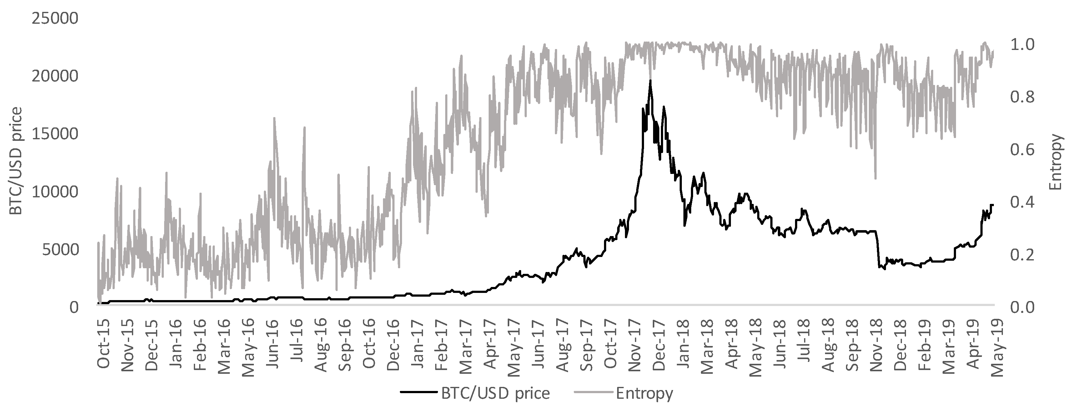
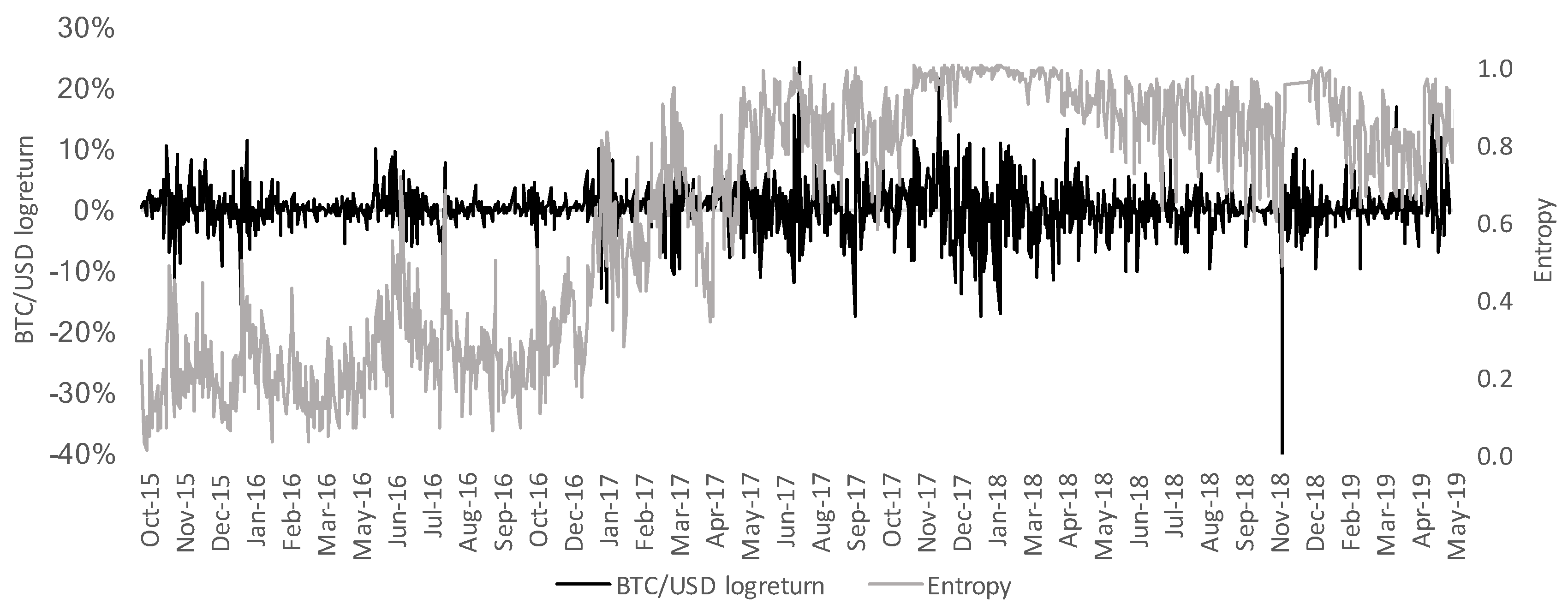
3.1. Bitcoin

There are several time series prices for Bitcoin depeding on the digital currency exchange and the currency used in the trading process. In order to compare our results to that obtained by Pele and Mazurencu-Marinescu-Pele [11], we adopt the BTC/USD exchange rate from Gemini Trust Company, LLC (Gemini). Gemini is a digital currency exchange and custodian that allows customers to buy, sell, and store digital assets. In particular, we consider the intraday closing prices of the minute-by-minute time bins and the time period from 8 October 2015 until 29 May 2019. According to Feng et al. [19] apud Pele and Mazurencu-Marinescu-Pele [11], the market capitalization, the daily transaction volume and the liquididy of Bitcoin before 2015 was not good.

For illustration purposes, in Figure 1, we present the Bitcoin’s daily closing prices; in Figure 2, we present the Bitcoin’s daily close-to-close logreturns; and, finally, in Figure 3, we present the empirical probability density and cumulative distribution functions of the Bitcoin’s daily close-to-close logreturns. It is possible to notice the huge increase in the Bitcoin’s prices until the end of 2017, the high volatility of the Bitcoin’s logreturns and the change over time of the volatility pattern. In addition, it is also possible to notice the existence of extreme values in the distribution of Bitcoin’s logreturns. In the following sections, we present the entropy of the symbolic intraday distribution of Bitcoin’s logreturns, the logistic model connecting the daily CVaR and the entropy, and a forecasting model for the daily CVaR using the entropy based on a modified quantile regression model.

3.2. Entropy and Daily CVaR

In Figure 1 and Figure 2, we also present the entropy of the symbolic intraday distribution of Bitcoin’s logreturns. As it was mentioned in Section 2, the entropy of the symbolic intraday logreturns is higher at the presence of higher uncertainty in the returns and lower at the presence of lower uncertainty in the returns. In [9,11], they have tested the hypothesis that the daily logprice of Bitcoin is positively correlated to the entropy of the symbolic intraday distribution of Bitcoin’s logreturns. However, we state that the logprice time series because of its level, non-stationarity and trend cause possible problems to the hypothesis verification. Consequently, we test the following model:

$$\left|r_d\right|=a_0+a_1{h}_d+{\epsilon }_d,$$

(19)

where ${\epsilon }_d$ is the error term. Our hypothesis about Equation (19) is that the absolute value of daily logreturn of Bitcoin is positively correlated to the entropy of the symbolic intraday distribution of Bitcoin’s logreturns. The estimation results of Equation (19) are shown in

Table 1. Estimation results of Equation (19).

Parameter	Estimation	p-Value	Standard Error
$a_0$	0.006	0.000	0.005
$a_1$	0.032	0.000	0.008
$R^2$	0.132

. It is possible to notice that the estimated coefficient $a_1$ of the entropy is positive and significant supporting our hypothesis.

In this paper, we propose the study of the relation between entropy of the symbolic intraday distribution of Bitcoin’s logreturns and the likelihood of extreme negative daily logreturns represented by the daily CVaR using Equation (8). The estimation results are shown in

Table 2. Estimation results of Equation (8) for $\alpha =1\%$.

Parameter	Estimation	p-Value	Standard Error
$c_0$	−9.133	0.002	1.316
$c_1$	8.253	0.001	3.488

and

Table 3. Estimation results of Equation (8) for $\alpha =5\%$.

Parameter	Estimation	p-Value	Standard Error
$c_0$	−6.961	0.001	0.592
$c_1$	7.800	0.001	1.605

for $\alpha =1\%$ and $\alpha =5\%$, respectively. It is possible to notice that the estimated coefficients $c_1$ of the entropy for both $\alpha =1\%$ and $\alpha =5\%$ are positive and significant supporting the hypothesis that entropy is positively correlated to the likelihood of extreme values of daily logreturns.

3.3. Forecasting Daily CVaR

Let ${\widehat{\mathrm{CVaR}}}_{\alpha ,{\mathcal{W}}_w\left(k\right)}$ be the historical daily CVaR at the significance level $\alpha$ calculated in the time window ${\mathcal{W}}_w\left(k\right)$. The forecasting model for the daily CVaR${}_{\alpha }$ at day $k+w+1$ using ${\widehat{\mathrm{CVaR}}}_{\alpha ,{\mathcal{W}}_w\left(k\right)}$ is given by:

$${\widehat{\mathrm{CVaR}}}_{\alpha ,k+w+1}={\widehat{\mathrm{CVaR}}}_{\alpha ,{\mathcal{W}}_w\left(k\right)}.$$

(20)

In order to study the forecasting performance of the daily CVaR${}_{\alpha }$, we estimate Equations (16) and (20) using a rolling window approach with a window length $w=250$ trading days. For comparison purposes, in

Table 4. Backtest results of daily CVaR at the significance level $\alpha =1\%$.

Model	MAE	RMSE
Forecasting using entropy	5.26 × 10${}^{-5}$	7.28 × 10${}^{-4}$
Forecasting using historical CVaR	3.56 × 10${}^{-4}$	4.52 × 10${}^{-3}$

and

Table 5. Backtest results of daily CVaR at the significance level $\alpha =5\%$.

Model	MAE	RMSE
Forecasting using entropy	1.04 × 10${}^{-4}$	5.42 × 10${}^{-4}$
Forecasting using historical CVaR	3.16 × 10${}^{-4}$	1.51 × 10${}^{-3}$

, we present a backtest of models (16) and (20) for significance levels $\alpha =1\%$ and $5\%$, respectively. The performance of the models is compared with the historical daily CVaR at the significance level $\alpha$ calculated in the time window ${\mathcal{W}}_w\left(k+1\right)$. In particular, we consider the mean absolute error (MAE) and the root mean squared error (RMSE) between ${\widehat{\mathrm{CVaR}}}_{\alpha ,k+w+1}$ and ${\widehat{\mathrm{CVaR}}}_{\alpha ,{\mathcal{W}}_w\left(k+1\right)}$. As it is possible to notice from our empirical results using Bitcoin, the use of entropy in the forecasting of the daily CVaR of the next day seems to be better than the naive use of the historical CVaR.

4. Conclusions

In this paper, we have two main contributions: a logistic model connecting the daily CVaR and the entropy, and a forecasting model for the daily CVaR using the entropy based on a modified quantile regression model. Basically, we extend the study performed by Pele and Mazurencu-Marinescu-Pele [11] to include the CVaR. In [9,11], they have tested the hypothesis that the daily logprice of Bitcoin is positively correlated to the entropy of the symbolic intraday distribution of Bitcoin’s logreturns. However, since the logprice time series is in level and presents a non-stationarity behavior and a trend, the verification of their hypothesis becomes infeasible. Consequently, the hypothesis we verify is that the absolute value of daily logreturn of Bitcoin is positively correlated to the entropy. In addition, we also verify that entropy is positively correlated to the likelihood of extreme values of Bitcoin’s daily logreturns using a logistic regression model based on CVaR and the use of entropy to forecast the Bitcoin’s daily CVaR of the next day performs better than the naive use of the historical CVaR.

References

- Rockafellar, R.T.; Uryasev, S.P. Optimization of conditional value-at-risk. J. Risk 2000, 2, 21–42. [Google Scholar] [CrossRef]
- Love, R.F.; Morris, J.G.; Wesolowsky, G.O. Facilities Location: Models & Methods; NY: North-Holland, The Netherlands, 1988. [Google Scholar]
- Sarykalin, S.; Serraino, G.; Uryasev, S.P. Value-at-risk vs. conditional value-at-risk in risk management and optimization. Tutorials Oper. Res. 2008, 270–294. [Google Scholar] [CrossRef]
- Yamai, Y.; Yoshiba, T. Comparative analyses of expected shortfall and value-at-risk: their validity under market stress. Monet. Econ. Stud. 2002, 20, 181–237. [Google Scholar]
- Rockafellar, R.T.; Uryasev, S.P. Conditional value-at-risk for general loss distributions. J. Bank. Financ. 2002, 26, 1443–1471. [Google Scholar] [CrossRef]
- Philippatos, G.C.; Wilson, C. Entropy, market risk and the selection of efficient portfolios. Appl. Econ. 1972, 4, 209–220. [Google Scholar] [CrossRef]
- Ebrahimi, N.; Maasoumi, E.; Soofi, E.S. Ordering univariate distributions by entropy and variance. J. Econ. 1999, 90, 317–336. [Google Scholar] [CrossRef]
- Dionisio, A.; Menezes, R.; Mendes, D.A. An econophysics approach to analyze uncertainty in financial markets: an application to the Portuguese stock market. Eur. Phys. J. B 2006, 50, 161–164. [Google Scholar] [CrossRef]
- Pele, D.T.; Lazar, E.; Dufour, A. Information entropy and measures of market risk. Entropy 2017, 19, 226. [Google Scholar] [CrossRef]
- Billio, M.; Casarin, R.; Costola, M.; Pasqualini, A. An entropy-based early warning indicator for systemic risk. J. Int. Financ. Mark. Inst. Money 2016, 45, 42–59. [Google Scholar] [CrossRef]
- Pele, D.T.; Mazurencu-Marinescu-Pele, M. Using high-frequency entropy to forecast bitcoins daily value at risk. Entropy 2019, 21, 102. [Google Scholar] [CrossRef] [PubMed]
- Zhang, W.; Wang, P.; Li, X.; Shen, D. Some stylized facts of the cryptocurrency market. Appl. Econ. 2018, 50, 5950–5965. [Google Scholar] [CrossRef]
- Hu, A.; Parlour, C.A.; Rajan, U. Cryptocurrencies: stylized facts on a new investible instrument. Work. Pap. 2018. [Google Scholar] [CrossRef]
- Saa, O.T.; Stern, J.M. Auditable Blockchain Randomization Tool. arXiv 2019, arXiv:1904.09500. [Google Scholar]
- Colucci, S. On Estimating Bitcoin Value at Risk: A Comparative Analysis. Work. Pap. 2018. [Google Scholar] [CrossRef]
- Daw, C.; Finney, C.; Tracy, E. A review of symbolic analysis of experimental data. Rev. Sci. Instrum. 2003, 74, 915–930. [Google Scholar] [CrossRef]
- Shannon, C.E. A mathematical theory of communication. Bell Syst. Tech. J. 1948, 27, 379–423. [Google Scholar] [CrossRef]
- Koenker, R.; Bassett, G. Regression quantiles. Econometrica 1978, 46, 33–50. [Google Scholar] [CrossRef]
- Feng, W.; Wang, Y.; Zhang, Z. Can cryptocurrencies be a safe haven: A tail risk perspective analysis. Appl. Econ. 2018, 50, 4745–4762. [Google Scholar] [CrossRef]