Some Effects of Crosswind on the Lateral Dynamics of a Bicycle †


Abstract
:1. Introduction
2. Methods
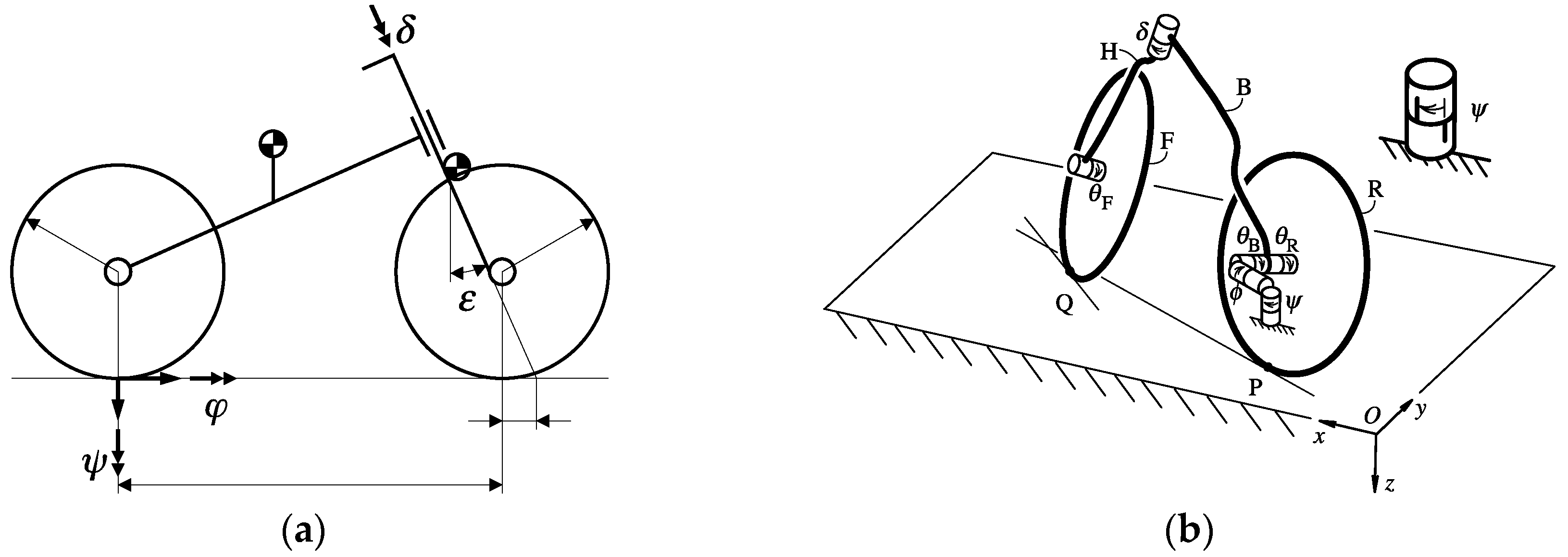
2.1. Bicycle Model
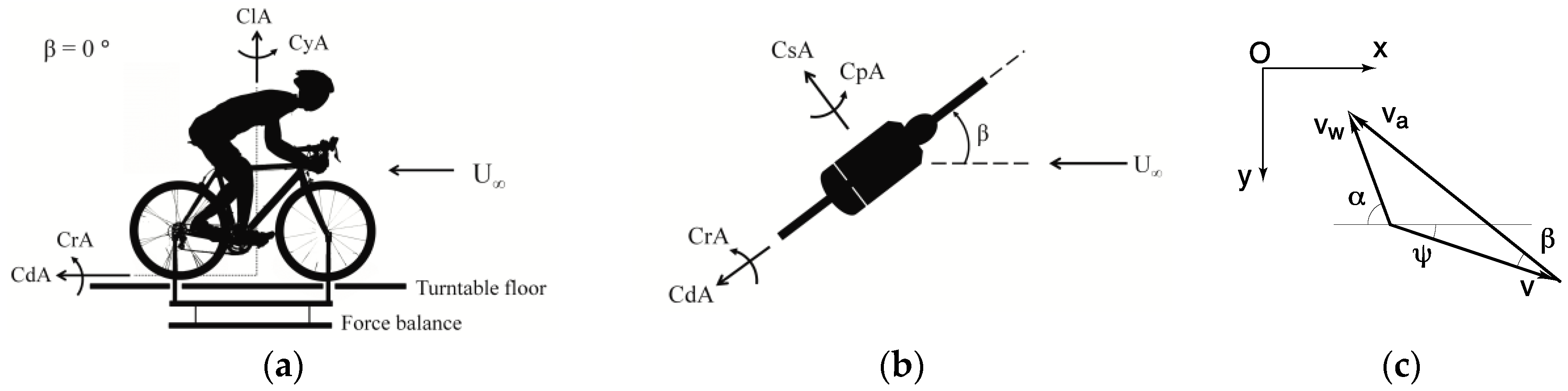
2.2. Cross Wind
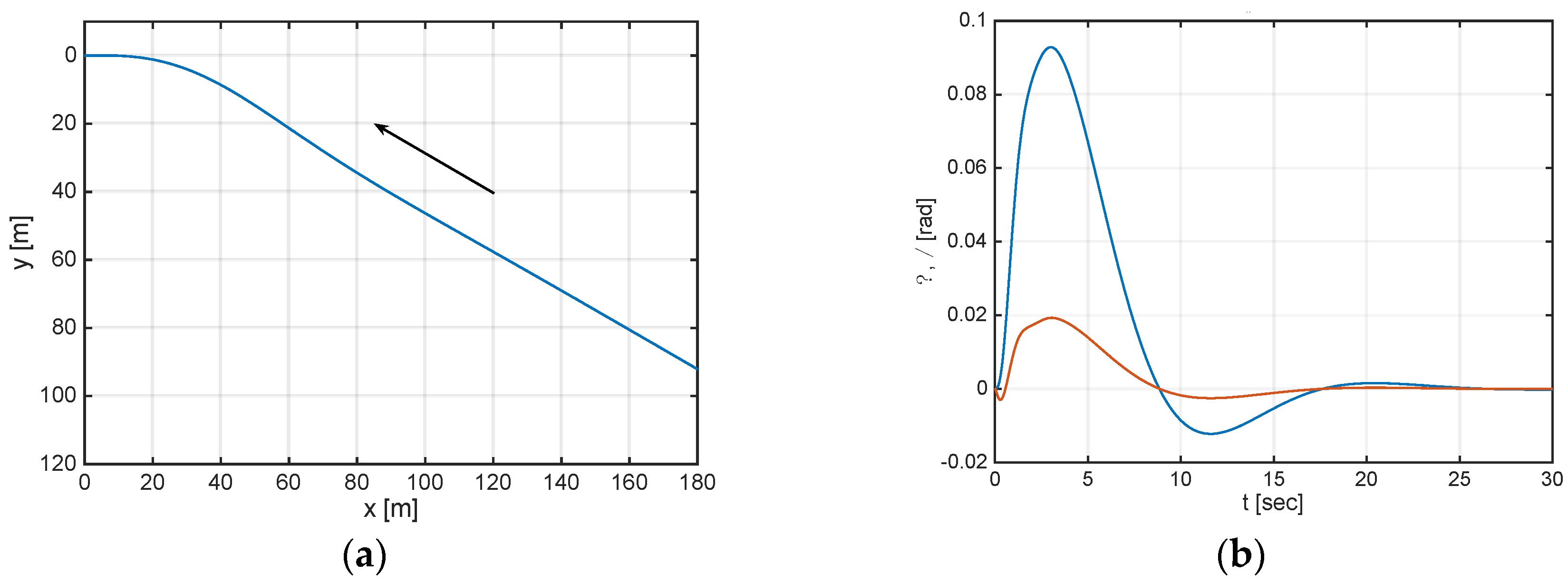
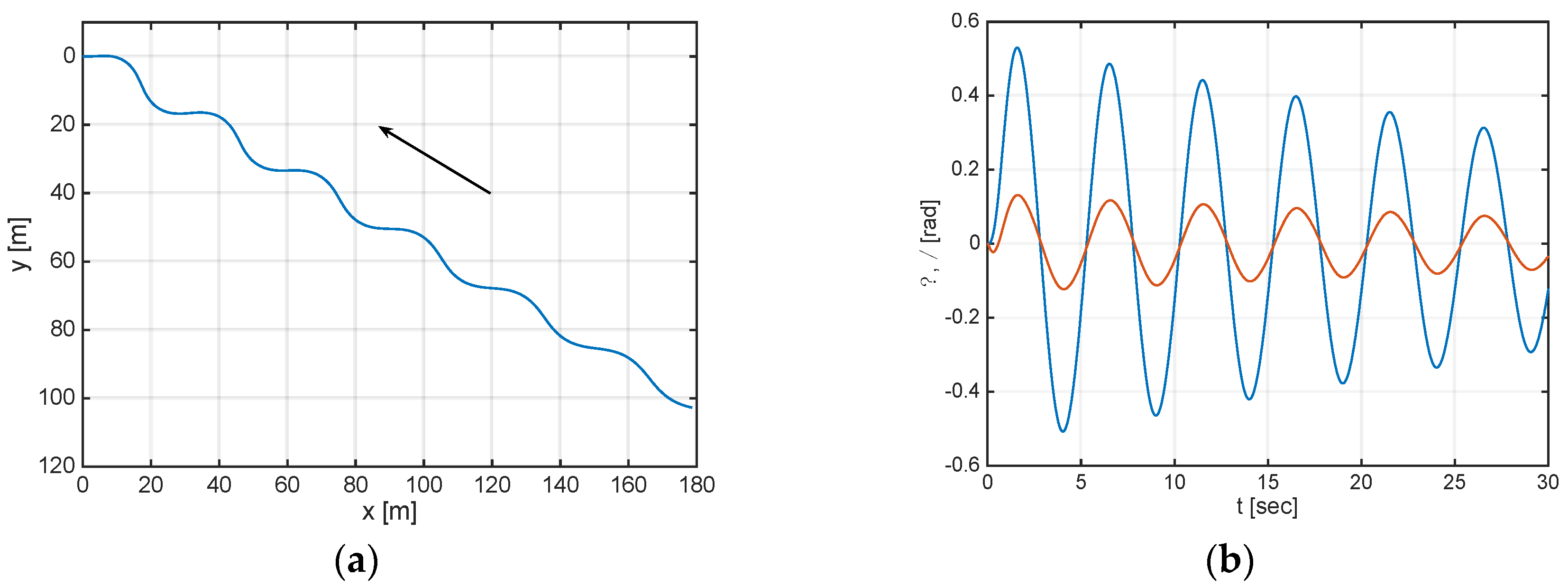
2.3. Time Series
2.4. Rider Control
3. Results and Discussion
4. Conclusions
Acknowledgments
Appendix A

References
- Debraux, P.; Grappe, F.; Manolova, A.V.; Bertucci, W. Aerodynamic drag in cycling: Methods of assessment. Sports Biomech. 2011, 10, 197–218. [Google Scholar] [CrossRef] [PubMed]
- Godthelp, J.; Buist, M. Stability and Manoeuvrability Characteristics of Single Track Vehicles; Tech. Rep. IZF 1975 0-2; TNO Institute for Perception: Soesterberg, The Netherlands, 1975. [Google Scholar]
- Barry, N.; Burton, D.; Crouch, T.; Sheridan, J.; Luescher, R. Effect of crosswinds and wheel selection on the aerodynamic behavior of a cyclist. Procedia Eng. 2012, 34, 20–25. [Google Scholar] [CrossRef]
- Barry, N.; Burton, D.; Sheridan, J.; Thompson, M.; Brown, N.A.T. Aerodynamic drag interactions between cyclists in a team pursuit. Sports Eng. 2015, 18, 93–103. [Google Scholar] [CrossRef]
- Belloli, M.; Giappino, S.; Robustelli, F.; Somaschini, C. Drafting Effect in Cycling: Investigation by Wind Tunnel Tests. Procedia Eng. 2016, 147, 38–43. [Google Scholar] [CrossRef]
- Blocken, B.; Toparlar, Y. A following car influences cyclist drag: CFD simulations and wind tunnel measurements. J. Wind Eng. Ind. Aerodyn. 2015, 145, 178–186. [Google Scholar] [CrossRef]
- Blocken, B.; Toparlar, Y.; Andrianne, T. Aerodynamic benefit for a cyclist by a following motorcycle. J. Wind Eng. Ind. Aerodyn. 2016, 155, 1–10. [Google Scholar] [CrossRef]
- Kyle, C.R.; Weaver, M.D. Aerodynamics of human-powered vehicles. Proc. Inst. Mech. Eng. Part A J. Power Energy 2004, 218, 141–154. [Google Scholar] [CrossRef]
- Schepers, P.; Wolt, K.K. Single-bicycle crash types and characteristics. Cycl. Res. Int. 2012, 2, 119–135. [Google Scholar]
- Meijaard, J.P.; Papadopoulos, J.M.; Ruina, A.; Schwab, A.L. Linearized dynamics equations for the balance and steer of a bicycle: A benchmark and review. Proc. R. Soc. A 2007, 463, 1955–1982. [Google Scholar] [CrossRef]
- Fintelman, D.; Sterling, M.; Hemida, H.; Li, F.-X. The effect of crosswinds on cyclists: An experimental study. Procedia Eng. 2014, 72, 720–725. [Google Scholar] [CrossRef]
- Schwab, A.L.; de Lange, P.D.L.; Happee, R.; Moore, J.K. Rider control identification in bicycling using lateral force perturbation tests. Proc. Inst. Mech. Eng. Part K J. Multi-Body Dyn. 2013, 227, 390–406. [Google Scholar] [CrossRef]
- Meijaard, J.P. The loop closure equation for the pitch angle in bicycle kinematics. In Proceedings of the Bicycle and Motorcycle Dynamics 2013 Symposium on the Dynamics and Control of Single Track Vehicles, Narashino, Japan, 11–13 November 2013. [Google Scholar]
- Moore, J.K.; Kooijman, J.D.G.; Schwab, A.L.; Hubbard, M. Rider motion identification during normal bicycling by means of principal component analysis. Multibody Syst. Dyn. 2011, 25, 225–244. [Google Scholar] [CrossRef]


Publisher’s Note: MDPI stays neutral with regard to jurisdictional claims in published maps and institutional affiliations. |
© 2018 by the authors. Licensee MDPI, Basel, Switzerland. This article is an open access article distributed under the terms and conditions of the Creative Commons Attribution (CC BY) license (https://creativecommons.org/licenses/by/4.0/).
Share and Cite
Schwab, A.L.; Dialynas, G.; Happee, R. Some Effects of Crosswind on the Lateral Dynamics of a Bicycle. Proceedings 2018, 2, 218. https://doi.org/10.3390/proceedings2060218
Schwab AL, Dialynas G, Happee R. Some Effects of Crosswind on the Lateral Dynamics of a Bicycle. Proceedings. 2018; 2(6):218. https://doi.org/10.3390/proceedings2060218
Chicago/Turabian StyleSchwab, A. L., George Dialynas, and Riender Happee. 2018. "Some Effects of Crosswind on the Lateral Dynamics of a Bicycle" Proceedings 2, no. 6: 218. https://doi.org/10.3390/proceedings2060218
APA StyleSchwab, A. L., Dialynas, G., & Happee, R. (2018). Some Effects of Crosswind on the Lateral Dynamics of a Bicycle. Proceedings, 2(6), 218. https://doi.org/10.3390/proceedings2060218