A Comparative Analysis of Windowing Approaches in Dense Sensing Environments ^†

Abstract

Windowing is an established technique employed within dense sensing environments to extract relevant features from sensor data streams. Among the established approaches of Explicit, Time-based and Sensor-Event based windowing, Dynamic windowing approaches are beginning to emerge. These dynamic approaches claim to address the inherent shortcomings of the aforementioned established approaches by determining the appropriate window length for live sensor data streams in real-time, thereby offering the potential to optimize and increase the recognition of these sensor represented activities. Beyond these potential benefits, dynamic approaches can also support anomaly detection by actively uncovering new, unknown window patterns within a trained model. This paper presents findings from a study which utilizes data from a single source dataset, towards benchmarking and comparing more traditional windowing approaches against a dynamic windowing approach. The experiments conducted on a real-world smart home dataset suggest Time-based windowing is the best approach. Through evaluation of results, Dynamic windowing approaches may benefit from carefully annotated datasets.

1. Introduction

Drivers for pervasive computing include increased battery, processing power and connectivity capabilities. Pervasive computing for healthcare solutions, in particular, are increasing due to the growth in the aging population, leading to more age-related diseases and raising health costs significantly [1]. Smart Environments are among the main application areas benefiting from pervasive computing and comprise a large set of sensors, actuators, displays and computational elements to enable them to “acquire and apply knowledge about the environment and its inhabitants in order to improve their experience in that environment” [2]. This is typically realized through combined networks of sensors, which provides information on the inhabitant’s activities of daily living. Simple contact sensors and motion sensors can be used here to collect information on activities occurring around the home, such as doors and cupboards opening and closing, and people moving around the home. Activity Recognition is used to recognize these activities of daily living and interpret events taking place in a smart home [3]. These activity recognition systems use this contextual information to understand the behaviors taking place within the environment [3,4]. As this information is personal and can identify different activities and behaviors about an individual’s personality, it is difficult to extract this information [5]. Activity Recognition is now a well-researched pattern recognition problem that aims at identifying and classifying activities carried out from sensor data sources. Typically, the Activity Recognition Chain (ARC) involves several steps including Data Acquisition, Preprocessing, Segmentation, Feature Extraction, Dimensionality Reduction, and finally, Classification. Within the segmentation stage of the ARC, there is an opportunity to employ various windowing techniques, to partition the data and extract useful features that are viewed as being characteristic of the target activities to be recognized. The most common types of windowing techniques reported in the literature include: Explicit windowing, Time windowing, Sensor Event windowing and Dynamic windowing. Each approach offers respective advantages and disadvantages.

Explicit Windowing (EW): This is a two-step approach where in the first step, segments of data are fragmented into activities themselves, with the classification of the actual activities taking place in the second step. As this approach attempts to split the data into the activity portions, issues arise when trying to estimate the size of the explicit activity portion, as each person will carry out activities differently and humans tend to deviate from exact patterns in terms of time taken for an activity. Because this approach is a two-step process it also means the second step is dependent and must wait for the first step to be completed [6].

Time Windowing (TW): This approach breaks the dataset into equal periods of time to segment the data. This approach is favorable when using streamed data as the sensors fire continuously in time. Issues with this approach occur when trying to choose the optimal period of time, as there may be too little data to represent an activity, or too much data spread across one window, influencing potentially more than one activity to represent this window. This issue is common in smart home data using binary sensors, as they do not have a sampling rate and often provide little information in short time windows. This approach is typically used for accelerometers and gyroscopes to divide exercise-based activities such as walking, running and jumping. This approach will be investigated further throughout the paper, discussing the advantages and disadvantages when applied to smart home data with other traditional approaches based on the experiments carried out [6,7].

Sensor Event Windowing (SEW): This approach splits the dataset into equal segments of sensor events fired. The advantage of this approach is that the windows will vary in time. Issues arise when busy or quiet periods occur, as there may be too much or too little context from fired sensors to represent an activity accurately. For example, in one window there may be sensors representing someone using the bathroom and sleeping, where sleeping sets off a small number of sensors, but has a much more significant time frame [6,8].

Dynamic Windowing (DW): DW allows for the window size to increase or decrease in length based on a set of identified rules and thresholds. In doing so, this approach aims to maximize the probability of a specific activity, per window. Using this approach, issues can occur if the source dataset contains portions of the data are not annotated correctly (or annotated at all), making it more difficult to correctly identify and classify the target activities. Furthermore, an additional downfall when using this approach is the inefficiency to model complex activities [9,10,11].

This paper presents findings from a comparison of windowing approaches, applied to a single data source. Previous researchers [7,8,9,10,11,12] have compared various windowing techniques pair-wise, however, there does not appear to have been a direct comparison based on a single dataset from which to benchmark and objectively compare results. This prompted the current study, to objectively benchmark a dynamic approach against older, more conventional approaches using a single data source.

The remainder of the paper is organized as follows: Section 2 discusses related works for each of the abovementioned windowing approaches. The experimental settings and dataset used is discussed in Section 3. Section 4 thoroughly describes the methodology of each of the approaches being investigated and how these were carried out. Section 5 discusses the results of the experiments, followed by Section 6 which summarizes this work in a conclusion with future work.

2. Related Works

Over the past number of years, a number of segmentation approaches have been investigated to support more robust Human Activity Recognition (HAR) within smart environments. These segmentation techniques are used to window (partition) the available data from which, relevant features pertaining to different target activities can be extracted. What follows is a brief review of established windowing techniques, employed to support HAR within smart environment settings.

EW is a two-step approach for segmenting activities in a data stream. Junker et al. use and EW approach to recognize sporadically occurring gestures in a continuous data stream from body-worn inertial sensors. They describe this approach as a natural partitioning of sensor signals for spotting tasks [13]. The first steps involved segmenting the sensor events into partitions, where each partition represents a potential activity. The second step involved classification of this segment of data representing the activity.

TW is regarded as a less computationally expensive approach than the EW process described above. TW is a common approach when the data source originates from accelerometer/gyroscope data as these provide time series data [7]. Oresti et al. carry out a review paper based on TW of time series data. They compare the impact different times have when carrying out different activities using accelerometers and gyroscopes [7]. Krishnan and Cook use a TW approach as a benchmark for an experiment on sensor event windowing [6]. Blond et al. investigate the effects of window length of the sensor data on varying sizes of datasets. They found the length of the window does not have a significant effect on the training and evaluation time of their algorithm, but the sample size has effects on the training time more [12]. Sannino, G. et al. use TW as part of a processing technique to detect falls [14,15]. Bashir et al. use TW and acceleration sampling frequency for HAR using a variable Activity Recognition (AR) duration strategy to improve energy efficiency and accuracy when using an accelerometer on a smart phone [16]. As the literature reviewed here mostly reflects TW for sampling data, it will be interesting to see how this approach compares to other windowing approaches on a binary dataset generated in a smart home.

SEW facilitates data to be segmented into windows of varying duration as they focus upon the events occurring within the data rather than the timing components of these events. Krishnan and Cook investigated the issues around busy or quiet periods within captured data streams and found that there were instances where too much or too little context is received from the sensor events, to represent an activity accurately. These experiments were carried out using smart home generated binary data, adding their own modifications to improve the shortcomings of this SEW approach.

In [6], the authors also experimented with a DW approach that uses statistics to determine the average window lengths of activities to carry out the DW, employing three CASAS testbed datasets. The results found that SEW was best in this case. Yala and Fergani extend upon the SEW approach used in [6], focusing on the Mutual Information (MI) aspect of this approach, where they use the most common sensor as the comparison point for the MI calculation as opposed to the last sensor event, also described as part of the approach in [8]. They achieved a 3%-point accuracy rise when using six weeks of the CASAS Aruba dataset. Based on these experiments, SEW proved to be the best windowing approach on smart home data so far [6].

Based on a review of the literature, DW is becoming an increasingly popular segmentation approach. Researchers such as Krishnan and Cook use a set of heuristics based on temporal and statistical information to define the DW sizes [6], as mentioned briefly above. This approach is then proved by Yala and Fergani, to be second best performing approach to their previously referenced extended features on a SEW approach [8]. Fahad et al. use a two-step approach with an offline phase and an online phase, where they define activities as a group, then use this information to dynamically monitor daily activities and detect anomalous behaviors [17]. Fatima et al. use sets of active sensors for related data to window data, using sequential behaviors from these classified activities to predict future and past activities [18]. Bernabucci et al. investigate the pre-processing effect on the accuracy of event-based activity segmentation using a dynamic event-based segmentation approach. However, they carry out the experiments using accelerometers for locomotion [19]. Fadi et al. also use a two-step approach for their DW approach, involving an offline phase and online phase. The offline phase is used to form a group of “best fitting sensors” for each activity, based on explicit windowed features and information gain to develop the most informative features for each activity. These “best fitting sensors” for each activity were then streamed online in the dataset using a custom algorithm to window the data based on these sensor groups firing. Statistical and spatial features were then extracted as inputs to support the classification of the activities contained within the dataset [9].

Each windowing approach reviewed offers a number of advantages and disadvantages as previously mentioned in Section 1. What is absent from the literature is an objective comparison of windowing approaches, based on experiments involving a single dataset. Consequently, it is not clear which windowing approach can be applied to best support HAR within smart environments. In this study, three different types of windowing approaches will be investigated by employing a single source dataset, in order to objectively investigate this problem.

3. Materials & Experimental Set Up

Dataset

The Aruba dataset, from the well-established CASAS project [20], was selected to evaluate and validate three different windowing techniques. 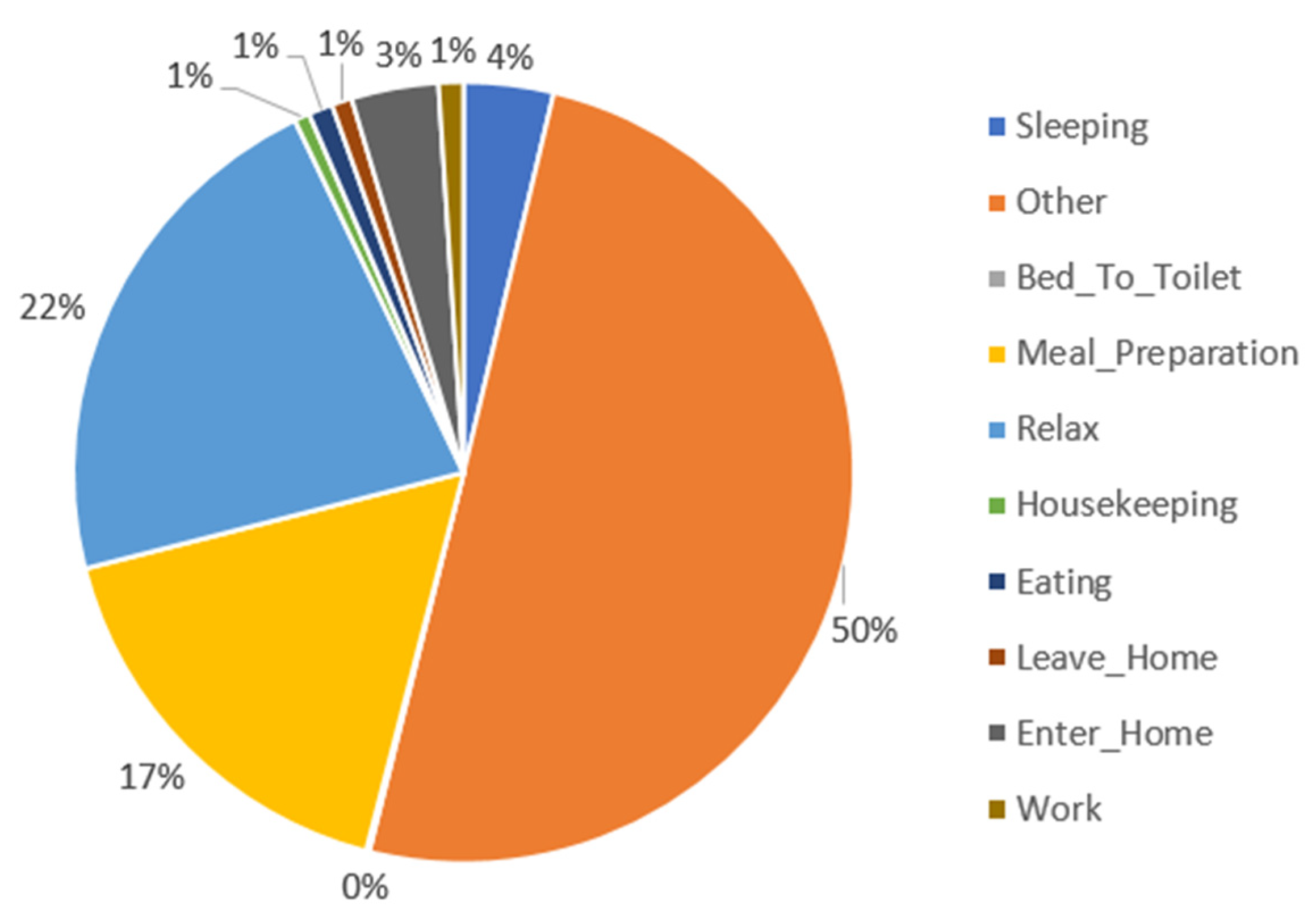This dataset was chosen as it has also been used in many previous experiments by other researchers to validate their research, specifically the DW approach that part of this experiment is based upon [9], and the worked based on the SEW approach in [6] that extends these features to achieve a higher classification accuracy [8]. The Aruba dataset was collected in the home of a single female adult occupant who undertook her normal daily routine for seven months that included regular visits from family members. There is a total of 11 different annotated activities represented within this dataset, as described in Figure 1. These are: Meal_Preparation, Relax, Eating, Work, Sleeping, Wash_Dishes, Bed_To_Toilet, Enter_Home, Leave_Home, Housekeeping, Respirate and Other. The dataset is reflective of a real-world activity set and exhibits class imbalance in the number of each activity represented. Furthermore, 50% of the dataset is annotated as ‘Other’, which related to missed annotations when the dataset was being collected, leaving the data unlabeled. There were 40 different sensors installed throughout the Aruba household, comprising: 31 binary motion sensors (PIR), represented in the data as “M001” through “M031”; four binary door sensors (“D001”…“D004”) and; five temperature sensors (“T001”…“T005”).

In the current study, Wash_Dishes and Respirate were removed for all of the experiments due to both having significantly under represented numbers of samples. The door sensor (D003) was removed as it is never triggered within the dataset and the temperature sensors (T001…T005) were also removed for each of the experiments as binary sensors were the focus for these experiments.

4. Methods

4.1. Time Windowing

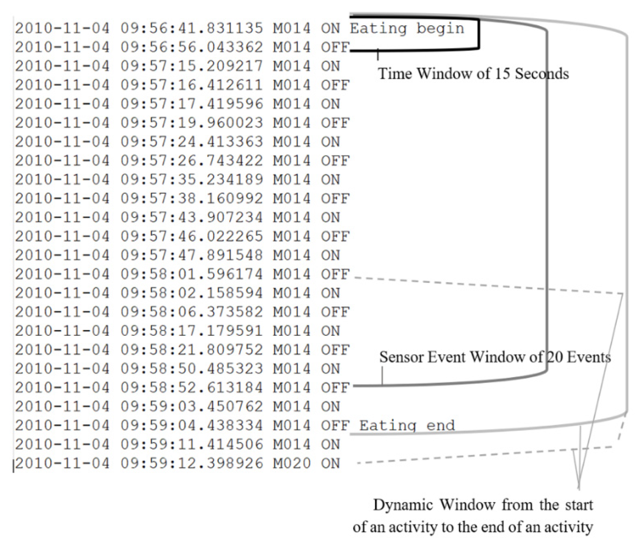
For the TW approach, the data was divided into equal time intervals. A time of 15 s was chosen, as previous literature suggests this as the optimal time to use for binary smart home data [6,21]. Figure 2 presents an equal time interval of 15 s in the Aruba dataset, represented by the black brace. For each window, several features were extracted, including the time of the first sensor event, the time of the last sensor event, the duration of the window, and a binary representation of every sensor, where “1” is displayed if a sensor has fired, and “0” is displayed if the sensor has not turned on within the TW segment.

4.2. Sensor Event Windowing

The SEW approach divides the data into equal sensor event intervals. Figure 2 presents a segment of 20 sensor events in the Aruba dataset that are represented by the dark grey brace, as the authors in [6] refer to 20 sensor events as the peak number of sensor events to use per window. As Krishnan and Cook expose, treating all sensor events with equal importance is not a good approach, as the last sensor event in some windows may belong as the first sensor event in the next window, and vice versa. Therefore, we base this approach on the SEW approach with extended features that gained the best results in [6]. The extra features in this case were referred to as MI and Previous Window Previous Activity (PWPA). MI is based on the chance of two sensors occurring consecutively within the entire window. This is calculated using a subset of the data. Then each field calculates the MI based on the current sensor in the window and the last sensor in the window each time, to set the feature value as the MI for that current sensor. PWPA is achieved using a two-step approach where the features space is firstly classified using LibSVM, a library for Support Vector Machines [22], and Platt’s scaling [23]. Predictions output from this first classification provide two new features: predicted class labels and the probability of this predicted label. Alongside these improved features, several other features were extracted from this window to form the final feature space. This included the time of the first sensor event, the time of the last sensor event, the duration of the window (in this case it will vary, one of the benefits of this approach), and instead of a binary representation of every sensor, similar to the TW approach, the MI value is used. Lastly, the previously mentioned predicted class label and probability of the next window are also used to generate a total of 40 features, in the final feature vector.

4.3. Dynamic Windowing

The DW approach presented here is based upon the work of Fadi et al. [9,10,11]. It involves a two-step approach with both an offline and online phase. In the offline phase, the raw dataset activities are windowed using the begin and end labels to extract a number of features, namely, number of activations of each sensor, sensor location, activation duration of each sensor and number of activated sensors. For example, for the activity ‘eat’, each of the abovementioned features are extracted from ‘eat begin’ to ‘eat end’ for the entire dataset and for each activity. Based on the features described above, the number of activations of each sensor was found to be the best feature using the Information Gain (IG) attribute evaluator in Weka [24] by averaging this rank for each of the features. The final feature space for this offline phase included the number of activations of each sensor and the class label. From the resulting set of features, the group of “best fitting sensors” was established using the IG, where sensors were added and removed iteratively based on the frequency of the activation times of all windows, resulting in the ‘best fitting sensor groups’, as shown in

Table 1. Best fitting sensor groups for each activity. “M001” … “M031” represent motion sensors and “D001”…“D004” represent door sensors throughout the Aruba Casas dataset.

Activity Class	Best Fitting Sensor Group
Sleeping	M003, M002, M007
Bed_To_Toilet	M004, M007, M005
Meal_Prep	M019, M018, M015, M017, M016
Relax	M009, M013, M020
Housekeeping	M031, M021, M008, M006, M005
Eating	M014, M009, M018
Leave_Home	M030, D004
Enter_Home	M030, D004
Work	M026, M027, M028

. A maximum of five sensors in a group was used to describe an activity, as shown in Table 1.

The online phase of the DW approach was carried out using the best fitting sensor groups for each activity. The best fitting sensor groups were incorporated into an algorithm that streams the entire dataset, windowing the nine activities based on these “best fitting sensor groups”. When a sensor fired, the best fitting sensor groups containing the current sensor, updated its value to “1”. When the algorithm identified a “best fitting sensor group”, where all sensors are set to “1”, this segment of data was identified and labeled as a single window for that activity. The frequency of each sensor fired within a single activity was used to produce an occurrence histogram, from which statistical features were extracted, namely: mean, median, standard deviation, skewness and kurtosis. These features were used to form the final feature space to be classified, along with the dynamically windowed activity label. Figure 2 presents the DW approach where the light grey brace represents the dynamic segment. The dotted grey braces represent the dynamicity of the approach which moves according to the best fitting sensor group that has fired.

4.4. Classification

All experiments employed a five-fold cross validation strategy, which were normalized before classification. LibSVM [22] was used for classification of activities in all of the experiments conducted.

5. Results

Table 2. Results for each of the windowing approaches.

Precision			Recall			F-Measure			Class
TW	SEW	DW	TW	SEW	DW	TW	SEW	DW
0.805	0.894	0.699	0.836	0.759	0.980	0.820	0.818	0.816	Sleeping
0.740	0.737	0.814	0.764	0.855	0.555	0.752	0.555	0.660	Other
0.000	0.000	0.000	0.000	0.000	0.000	0.000	0.000	0.000	Bed_to_Toilet
0.678	0.773	0.623	0.799	0.680	0.764	0.734	0.673	0.687	Meal_Preparation
0.872	0.816	0.543	0.873	0.817	0.859	0.873	0.765	0.665	Relax
0.000	0.000	0.000	0.000	0.000	0.000	0.000	0.000	0.000	Housekeeping
0.000	0.614	0.000	0.000	0.306	0.000	0.000	0.430	0.000	Eating
0.000	0.683	0.000	0.000	0.331	0.000	0.000	0.473	0.000	Leave_Home
0.000	0.898	-	0.000	0.071	-	0.000	0.248	-	Enter_Home
0.558	0.670	0.000	0.796	0.348	0.000	0.656	0.479	0.000	Work
0.740	0.764	0.698	0.772	0.764	0.666	0.755	0.746	0.657	Weighted Average

presents the results from the experiments involving the three windowing approaches. Results from TW showed a weighted average F-Measure of 0.755. Most correctly identified activities, based on F-Measure for the TW approach are Relax (0.883), Sleeping (0.818), Meal_Preparation (0.734) and Work (0.656). Relax has the highest precision and recall, followed closely by sleeping, and Meal_Preparation. Some activities were not classified at all, such as Bed_To_Toilet, Housekeeping, Eating, Leave_Home and Enter_Home, which all had an F-Measure of 0.00. Relax, Sleeping and Meal_Preparation are the most accurately classified activities.

SEW results show a weighted average F-Measure of 0.746. Most correctly identified activities, based on F-Measure for the SEW approach, were found to be Sleeping (0.818), Relax (0.765) and Meal_Preparation (0.673). Other, less well classified activities based on F-Measure are Work (0.479), Leave_Home (0.473), Eating (0.430) and Enter_Home (0.248). Most incorrectly identified activities were Housekeeping and Bed_To_Toilet, that both resulted in an F-Measure of 0.00. SEW has the highest classification for Eating, Leave_Home and Enter_Home, and this is the only approach to classify these activities from all of three of the approaches carried out in the experiments.

DW results present a weighted average F-Measure of 0.657. Most correctly identified activities, based on F-Measure for this approach are Sleeping (0.816), Relax (0.665), Meal_Preparation (0.673) and Other (0.660). Other has the highest precision for the DW of all the approaches compared, whereas the other best identified activities in this approach, Sleeping, Meal_Preparation and Relax, have dropped precision, in comparison to the TW and SEW approach. All other activities for this approach were not classified with an F-Measure of 0.00. Enter_Home was consumed in the online windowing phase of this approach and is represented as “-” in the table.

6. Discussion

Based on the TW results, it was found that a number of activities are not classified. This may be due to lack of instances for some classes to be trained, such as Bed_To_Toilet and Housekeeping. However, TW does have the highest precision of the class Relax in comparison with the other two approaches. Although this approach has the highest overall accuracy and weighted F-Measure for all of the classified activities, it only classifies half of the activities within this dataset, which is not desirable in a real-world environment.

The SEW approach provided the next highest result, as shown in

Table 3. Accuracy of each of the windowing approaches.

Windowing Approach	Accuracy (%)
TW	77.20
SEW	76.39
DW	66.65

, with an accuracy of 76.39% and weighted F-Measure of 74.6. This is the only approach out of all three approaches to classify Eating, Leave_Home and Enter_Home. This approach also resulted in the highest precision for classes Sleeping, Meal_Preparation, Eating, Leave_Home and Enter_Home. In the first step of this approach without the PWPA features, previously mentioned in Section 4.2, the activities were classified at 70.21%. In the second step of this approach which includes the PWPA features, the classification results were 76.39%, resulting in an increase in accuracy of 6.02%. The F-Measure rose from 68.60 in the first step to 74.60 after the second step. As noted in Section 4.2, the second step in this approach used predicted labels and probabilities of these predictions as extra features to the feature space. As a result of these features, the second step has overwritten the Bed_To_Toilet class, which was classified correctly in the first step of the approach, but then later unclassified through this prediction step. This is because the PWPA feature never predicts Bed_to_Toilet. If more Bed_To_Toilet cases were available in a dataset, it is postulated that this activity may also be correctly classified more often within the dataset.

The DW results indicate that only some of the activities in the dataset are classified when streamed. It is postulated to be due to the iterative approach used to find the best fitting sensor groups for the DW approach and the high percentage of the Other class in the dataset. Using the iterative approach described in the methodology, the activity Enter_Home was consumed in the online phase of the approach. This is because the same sensor group is used for both Enter_Home and Leave_Home based on their IG values, therefore only one activity will be labelled when this sensor group fires, in this case Leave_Home being labelled and Enter_Home being consumed. This problem may be avoided in future if the window of temporary sensors is kept “open”, to evaluate which activity is more likely, based on the best sensor group that appears in the data stream. The DW approach produced the highest precision for the class ‘Other’, which implies the DW approach may have a greater impact in tasks such as anomaly detection, as it is assumed that the ability to detect non-labelled tasks could potentially offer a benefit within the anomaly detection research area. The DW approach may also perform better in real-time as it may have less instances to traverse through in order to find an activity. For example, the TW approach must run through 15 s of sensor data before producing a window, the SE approach must run through 20 sensor events before producing its first window, but, the DW approach may not always have to wait this long before producing its activity windows.

When looking at each of the results in Table 2 and Table 3, it is clear that in terms of accuracy, TW is the best approach, resulting in an accuracy of 77.2%, followed by SEW (76.39%) and then the DW approach (66.65%). As the dataset used to carry out these experiments is unbalanced, with 50% of the dataset being classed as Other, accuracy is not regarded as a fair measurement to use as it may mislead the results in such an unbalanced dataset. F-measure is a more suitable metric as it shows how well each activity performs, taking into account the precision and recall., of how each activity performs. When using F-Measure as the evaluation metric, the TW approach produced the highest result for the activities it classifies, Sleeping, Other, Meal Preparation and Relax, however, this is only half of the activities from the dataset. The F-Measure of these activities for the TW approach are followed closely by the SEW approach, however, the SEW approach also classifies four other activity classes, namely, Eating, Leave_Home, Enter_Home and Work, making this the best performing approach based on classifying more activities than the TW approach and with only a slightly lower F-Measure for all other activities.

The DW approach adopted for these experiments performed less well than the other two approaches. This is at odds with the original hypothesis of this study. Based on accuracy, the DW approach scores 66.65%, the lowest scoring of the approaches experimented, with only four activities being classified using this approach, whereby each scored lower than when using the other windowing approaches. Nevertheless, there are areas for improvement with this approach that could be investigated, such as the use of statistical features in the DW approach and not in the TW or SEW approaches, the real-time performance this approach achieves, the overfitting influence of the ‘Other’ class within the dataset and, the potential to pair this DW approach with anomaly detection, which all make this an interesting area to research further.

7. Limitations

The Aruba dataset chosen for this study contains seven months of free-living data, which is large in size in comparison to other smart home datasets. The methodology presented in this paper has a shortcoming in only considering this one dataset, however, the use of additional datasets would support the results and improve the robustness of the methodologies. In future more than one dataset should be used, such as the Opportunity dataset [25], or other datasets from the CASAS testbed, such as Tulum or Kyoto [21].

Another limitation of the Aruba dataset is that it is heavily imbalanced. Each windowing approach suggests that this class imbalance influences the results negatively for each activity with fewer instances. If a balanced dataset were used, it is hypothesized that these activities that perform poorly due to suspected lack of instances, would perform much better.

As the Aruba dataset is a free-living dataset, not all sensor events are annotated or annotated correctly, which could be due to human error, such as forgetting to finish or start an activity annotation. The Aruba dataset has 50% unannotated data that is labelled as “Other”. This is a clear limitation when using the DW approach with this dataset as the DW approach has a disadvantage against the other windowing approaches, as it can only ever assign a label for ‘known activities’ within the dataset. Future work will remove and compare the approaches without the unannotated data, or find a way to incorporate such unannotated data within the DW approach.

8. Conclusions

In this paper we reviewed three different types of windowing approaches: time windowing, sensor event windowing, and dynamic windowing. We reviewed at each of the advantages and disadvantages of these approaches. We directly compared the three approaches against one another using a single source dataset benchmarked using a single classifier. Subsequently, it was found that TW was the best approach in terms of accuracy and weighted F-Measure for the five of the activities but was lacking in classifying another four activities. The SEW approach was the next best approach based on accuracy and weighted F-Measure and additionally was able to classify a further three activities that TW approach does not. Lastly and somewhat unexpectedly, the DW approach only classified four of the nine activities in the dataset. This is rationalized by considering that the DW approach does not recognize “Other” as an activity and is therefore disproportionately disadvantaged in these experiments where “Other” accounts for 50% of the activity instances investigated. In terms of F-Measure, it is clear the SEW approach classifies the most activities in the dataset and all other activities classified by the SEW approach closely matched the F-Measures obtained by TW, therefore this may be considered as the best approach for use with smart home generated binary data, as used in these experiments.

In future work, the “best fitting sensor groups” for this DW approach will be explored further and additional DW approaches will be investigated. Dynamic approaches will also be investigated with the removal of unannotated data, alongside exploring ways to incorporate such unannotated data within the DW approach. A potentially interesting application of dynamic windowing is its application to anomaly detection within dense sensing environments, such as smart homes. Anomaly detection is an important research topic, not only for identifying unusual or unexpected activities within a smart home but for identifying infrequent activities within large imbalanced datasets. Consequently, it is anticipated that anomaly detection paired with an improved DW approach is a potentially useful and thought-provoking area to explore further.