The Predictability of Northern Hemispheric Blocking Using an Ensemble Mean Forecast System ^†

Abstract

Some weather extremes can be the result of atmospheric blocking, which can be responsible for the stagnation of weather patterns. These large-scale quasi-stationary mid-latitude flow regimes can result in significant temperature and precipitation anomalies in the regions that the blocking event impacts. The ability to predict periods of anomalous weather conditions due to atmospheric blocking is a major problem for medium-range forecasting. Analyzing the NCEP Ensemble 500-mb pressure heights (240 h) ten-day forecasts, and using the University of Missouri blocking archive to identify blocking event, the forecasted duration and intensity of model blocking events are compared to observed blocks. Comparing these differences using four case studies occurring over a one-year period across the Northern Hemisphere has shown the continued need for improvement of the duration and intensity of blocking events. Additionally, a comparison of the block intensity to a diagnostic known as the Integrated Regional Enstrophy (IRE) was performed in order to determine if there is a correlation between these quantities. Having a better understanding of knowing how long each block will last and their associated anomalies can help society prepare for the damage they can cause. Simulating and identifying blocks correctly is important in improving forecast issues.

1. Introduction

Previous work describes or defines atmospheric blocking in a number of different ways, including as a persistent height anomaly [1] or a weakness in the 500-hPa winds [2]. The work of [3] set forth a criterion that encompasses many blocking characteristics. A generic definition may be that blocking is a non-linear large-scale phenomenon that occurs in the atmospheric pressure field that results in a quasi-stationary steady state in the mid-latitude flow. Cyclonic wave breaking, which results in the upscale cascade of enstrophy, is important in the maintenance of mid-latitude weather and climate (e.g., [4]). This cyclonic wave breaking can contribute to a persistent blocking episode, which leads to above or below average temperature and precipitation anomalies over the surrounding area caused by stagnant weather patterns (e.g., [4]). Then [5,6] describe the relationship between developing upstream cyclones and the onset and /or maintenance of blocking in some detail including a description of the phase relationship between the large and synoptic-scale wave and the development of a jet maximum on the upstream flank of the blocking events.

Also, the work of [4,7], and many other studies examined the persistent and severe summer heat wave of 2010 over Eastern Europe and Russia. There were more than 50,000 deaths in Russia alone including more than 1600 people who drowned as they entered water to escape the heat. This heat wave caused large economic losses, as crops were damaged. An increase in wildfires and smog levels in major Russian cities led to severe illness as well. The heat wave was the result of three atmospheric blocking events that covered the Euro-Russian region lasting from late June to mid-August [7]. The low predictability of the models caused the under forecasting for extreme surface temperatures, and the timing for the decay and maintenance of the blocking events [4]. Since numerical models are reliable out to about seven days or so, but limited to 10–14 days at a maximum (e.g., [8,9]) the failure of these models in operational forecasting is a problem for anticipating blocking. Model predictions are subject to fail for various reasons, several being: parameterization errors, lack of data, measurement errors and errors in initial conditions (e.g., [10] and references therein).

Previous work on blocking predictability from [11] investigated the frequency, seasonal variability and predictability of blocking using only one model, the European Centre for Medium-Range Weather Forecasts (ECMWF). They analyzed a seven-year data set and expanding from previous work they decided to analyze for both the Northern and Southern Hemisphere year-round. The study found Atlantic blocking events to occur more in the spring while Pacific blocks were frequent in the winter with a weak peak in summer. Block intensities were estimated most faithfully in the spring, but was over-estimated in autumn. Blocking onset was less predictable in the winter and summer in comparison to spring. Persistent Atlantic blocks were predicted better when compared to persistent Pacific blocking events. They [11] also suggested that a small number of case studies would be needed in order to determine where models failed.

Then [12] performed a similar study to [11] on a 1985 winter European/Eastern Atlantic Ocean blocking event focusing on the predictability of blocking onset and the planetary/synoptic-scale conditions prior to blocking onset using forecast ensembles. They used an ensemble suite available through the Community Climate Model (CCM) group at the National Center for Atmospheric Research (NCAR). The ensemble consisted of ten members. Initial data and model error were still unclear determining factors in model accuracy. Understanding that planetary scale features are predictable in a relative sense to blocking motivated this study. Relaxing the criterion of [13] for blocking and setting different lead-times, the study of [12] found that with greater lead-times prior to blocking onset the less predictable blocking was in the individual ensemble members. All members failed to locate the block accurately due to model systematic errors at lead times greater than seven days. They [12] also concluded that neither planetary nor synoptic initial conditions were linked to uncertainty to a greater extent than the model bias or model systematic errors. This suggests that even if systematic errors were identified, model bias may not be eliminated.

Additionally [14] eliminated model bias in their study by calibrating the Global Spectral Model (GSM) of the National Centers for Environmental Prediction (NCEP) ensemble forecast. Using the technique of [15], or forecasting from different times for the same day, a probabilistic forecast could be created. Skill scores were calculated and tested for accuracy to create the calibrated forecast. Then for bias, the Heidke skill score (HSS) and false alarm rate (FAR) were utilized (see [16] for more details). The probabilistic calibrated forecast was compared to NCEP reanalysis and the un-calibrated ensemble forecast. They [14] concluded that probabilistic calibrated forecast compared to un-calibrated ensemble forecast showed great improvements, and these forecasts were close to reanalysis data over the Atlantic region. Due to lack of data in the Pacific region, the calibrated forecasts were not as successful. Then [14] only focused on blocking onset and frequencies during cool season from September–May 1959–1998 in both the Atlantic and Pacific region.

The work of [17] examined predictability in an ensemble forecast system using the Integrated Regional Enstrophy (IRE) technique originally formulated by [18]. Their test involved examining the time series of IRE and its derivative (DIRE) during the life cycle of two blocking events. They found that the ensemble mean performed better that the control forecast in representing these quantities, but individual ensemble members better correlated to the observed event regardless of the resolution of the analyses. However, none of these studies cited above examined the details of block onset as in [5] or block intensity.

As opposed to previous studies that examined climatological data sets with numerous blocking event, this study will be similar to [10] and analyze four quasi-randomly chosen blocking events during the period May 2016–2017 and representing Pacific and Atlantic Region as well as strong and weak blocking events. The National Meteorological Center (NMC—now NCEP) started operational ensemble forecasting during December 1992 [19]. Using National Centers for Environmental Prediction (NCEP) ensemble mean forecast and the NCEP/NCAR Reanalysis, a comparison between model and observed data will be made for the four blocks mentioned above. The study will focus on the ability of the model to predict blocking onset/decay, longevity, block intensity (BI—[20]), and location. This study will also examine a possible correlation between BI and IRE. It is hypothesized that the models will underestimate blocking intensity and decay while more accurately predicting longevity and location. Section two will discuss the data and methods used to perform this research; section three will examine the synoptic aspects of each blocking event as well as IRE; section four will compare the ensemble modeled blocking and observed data; and sections three and four will discuss the results.

2. Data and Methods

2.1. Data

Previous work has shown that ensemble forecasts perform well in predictability of high impact weather and the potential occurrence of it. Simulating blocking has greatly improved with the use of medium-range numerical weather prediction (NWP) models [4]. Instead of providing one model solution a range of possible solutions are given. When designing the ensemble model, a “probabilistic” approach was taken and used a lower-resolution (T62, equivalent to ~210 km) variation of the medium-range forecast (MRF) model [21]. The NMC (now NCEP) developed their own ensemble forecast that once had 14 members, but now provides 17 global forecasts that begin from nearly identical initial conditions. This ensemble forecast provides several different plots that can be used for medium range forecasting applications. One of these products used for this research is known as the “spaghetti” plot, which provides two contours from each of the ensemble member 500 hPa height field chosen to best represent the mid-latitude and subtropical flow. These ensembles mean plots consist of representative contours from the mean 500-hPa heights calculated from each member of the ensemble [19].

Datasets used for this study is provided by the NCEP Global Ensemble Forecast System (GEFS) ensemble mean forecast and the NCAR Reanalyses associated with four Northern Hemisphere blocking events from 2016 to 2017. From the ensemble forecast model this study used the Northern Hemisphere 500-hPa height fields (m) for the mean and spaghetti plots. These 500-hPa heights were analyzed for ten days (240 h) focusing on their location, duration and intensity in comparison to observed atmospheric blocking events.

The NCEP/NCAR (National Center for Atmospheric Research) Reanalyses are used for the observed data [22] and

Table 1. Information from [22]; specification for this research to download plots from the pressure section.

NCEP/NCAR Reanalysis 1: Pressure Level Section
Temporal Coverage	Spatial Coverage	Levels	Update Schedule
4-times daily, daily and monthly values for 01/01/1948 to present Long term monthly means, derived from data for years 1981–2010 Values are instantaneous at the time indicated in the files	2.5 degree × 2.5 degree global grids (144 × 73) 0.0 E to 357.5 E, 90.0 N to 90.0 S	17 pressure levels (mb): 1000, 925, 850, 700, 600, 500, 400, 300, 250, 200, 150, 100, 70, 50, 30, 20, 10 Some variable have less: omega (to 100 mb) and humidities (to 300 mb)	Daily 12z

shows the available information that can be obtained from the website. The data used here was the pressure level data specifically the 500 hPa heights (m) plotted on a 2.5° latitude by 2.5° longitude grid. These data are available from 1 January 1948 to the present. NCEP used the same climate model throughout, initialized with a wide variety of weather observations. Some of the observations used included ships, planes, station data, RAOBS (Radiosonde database), and GOES satellite observations just to name a few. Using one model eliminated the complications that model changes can cause when examining climate/weather statistics and dynamic processes [23].

2.2. Methods

In order to identify observed and model blocking events the criteria used in this study is the criteria of [5] which is the following:

• the criteria of [24] must be satisfied for an anticylonic flow region at 500 hPa with the exception that the minimum duration must be five days [25],
• a negative or small positive LO index [2] must be present on a Hovmöler diagram in the Northern Hemisphere,
• conditions 1 and 2 must be satisfied together from 24 h after onset to 24 h before termination,
• the anticyclone should be poleward of 35° N or 35° S and the ridge should have an amplitude of greater than 5° latitude,
• block onset is described to occur when condition 4 and or conditions 1 or 2 are met,
• termination is designated at the time the event fails condition 5 for a 24-h period or longer [20].

More information can be found in [2,20]. This criterion was used to determine the four blocks discussed in this study. The purpose of this study is to compare the model ensemble performance to observed events, in reference to the predictability of the blocking events longevity, onset and termination and intensity. In order to determine a blocking event intensity [3] introduced a quantity known as blocking intensity index (BI) and [20] modified BI for automated use. This quantity is defined as:

$$BI=\left(\frac{\frac{Center}{\left(\frac{lowest upstream+center}{2}\right)+\left(\frac{lowest downstream+center}{2}\right)}}{2}-1\right)\times 100$$

(1)

where each variable is a 500 hPa high value obtained from the blocking event. The intensity for blocking is proportional to the strength of mid-latitude height gradients. The stencil is similar in form to a second order one-dimensional Shapiro filter [26] (see also [5]. Also, the work of [20] defined a strong block as those with a BI larger than 4.3 units, and a weak block as those with a BI smaller than 2.0, and all others between these values as moderate.

In order to evaluate the preformance of the ensemble mean model, lead times beginning with seven days (168 h) prior to the observed event were examined. The results will summarise this by showing lead times of seven, four, and one day. Then the block intensity for the mode events was dervided in order to compare to onservations. This study will also discuss the the use of IRE and compare this quanitty to block intensity. IRE has been shown to be a useful diagnositic in identifying blocking and/or regime transition [17,27,28]. Also, the study by [18] describes blocking as a quasi-stationary atmospheric state with quasi-barotropic structure, and in a quasi-barotropic flow the sum of the positive Lyapunov exponents is related to IRE. A Lyapunov exponent is the measure of the divergence or convergence of system trajectories that are initially close, and can be approximated by integrating enstrophy over a finite region known as IRE, which is vorticity squared [10,29]. The work of [29] used this technique to determine the stability or predictability within a planetry flow regime.

IRE is calculated following [7], and defined as:

$$Enstrophy={{\displaystyle \sum }}_{{\lambda }_i>0}{\lambda }_i\approx {{\displaystyle \int }}^{ }{\zeta }^2$$

(2)

where ζ is the voricity or curl of the wind field. his value can be used as a mesure of predictability, higher values correspond to a lesser degree of predictabilty or possibly the transitioning of atmospheric flow, while lower values correspond to a greater degree of predictability in a more stable flow configuration (e.g., Lupo et al., 2012; Jensen and Lupo, 2014). In order to calculate this quantity, the geostrphic vorticity,${\zeta }_g=\frac{g}{f}{\nabla }^{2}z$ was used and differentials were calculated using second order finite differencing over a 20° latitude by 20° longitude grid box encompassing the center of the blocking event.

During the period May 2016–May 2017, there were 39 blocking events that occurred over the Northern Hemisphere [30], including 19 over the Atlantic, 13 over the Pacific, and seven over the continental regions as defined by [20]. Blocking events were selected to represent a diverse sample with respect to intensity, location, and seasonality within the Northern Hemisphere.

Table 2. Description of blocking events discussed. Name, date of event/longevity and blocking intensities from observed data. Intensities calculated are mean values over the duration of the blocking event daily.

#	Location (at Onset)	Date/Longevity	Observed Intensity
1	Atlantic (50° N 20° E)	12Z 23 June–00Z 8 July 2016	2.46
2	Pacific (50° N160° E)	00Z 27 August–00Z 4 September 2016	1.99
3	Atlantic (55° N 0°)	00Z 3 October–00Z 27 October 2016	3.94
4	Pacific (50° N 160° W)	00Z 23 February–00Z 16 March 2017	4.40

lists the blocks that are studied in this research and they will be referred to by their location and intensity in section three. Blocking event one is a relatively weak and short-lived Atlantic event, block two is a weaker and short-lived Pacific event, block three is a stronger and more persistent Atlantic event, and block four is a strong and persistent Pacific event. These events are of characteristic intensity with respect to the seasons in which they occur [20], and [5] demonstrated that there is a correlation between strength and duration. Thus, it is not surprising that this sample is reflective of this trait of blocking characteristics.

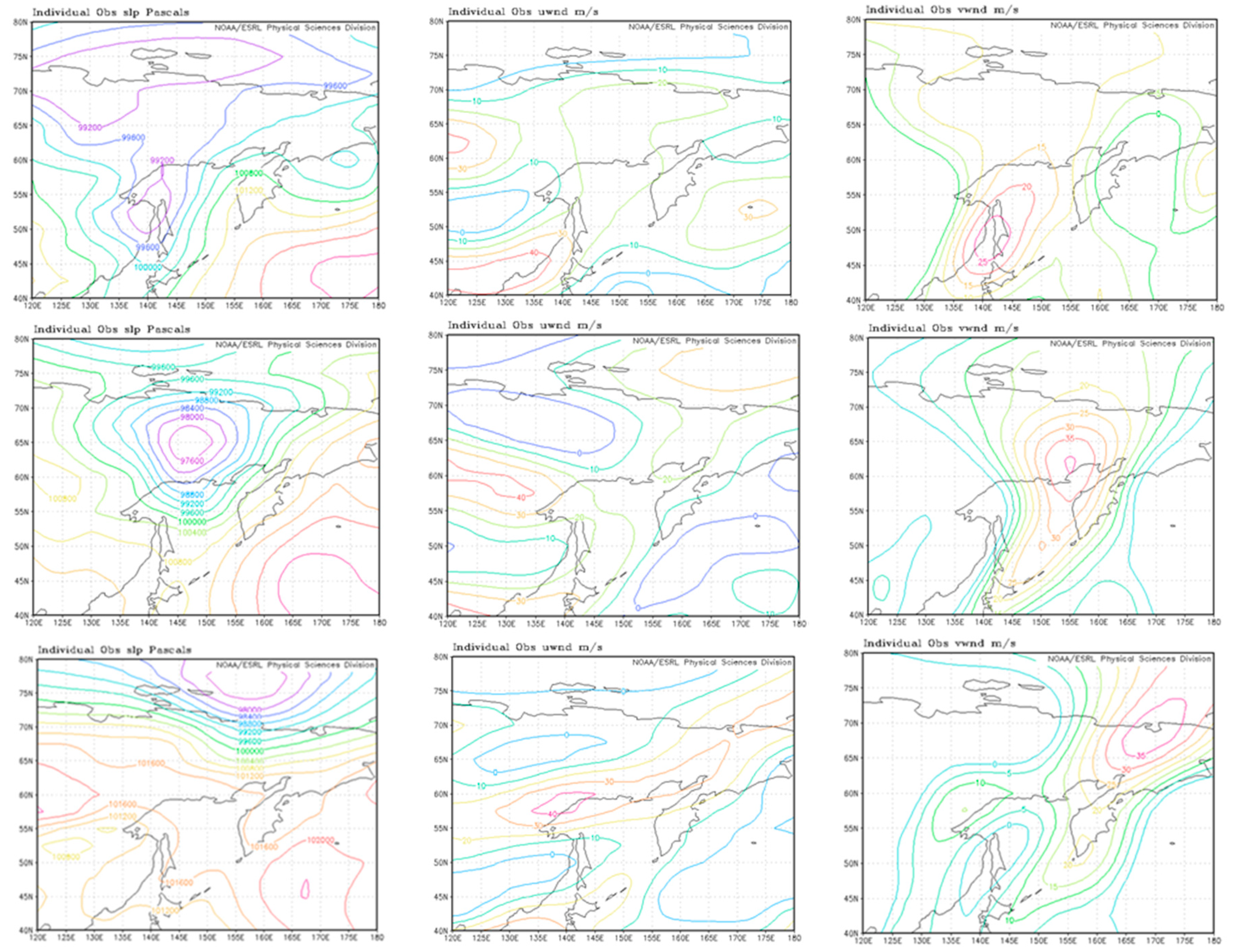
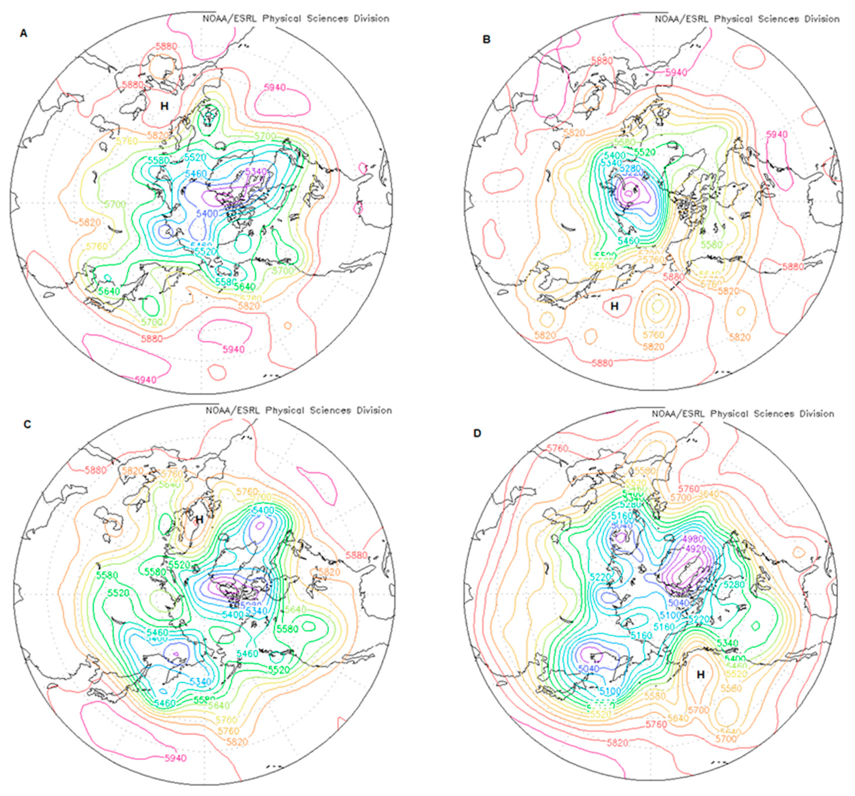
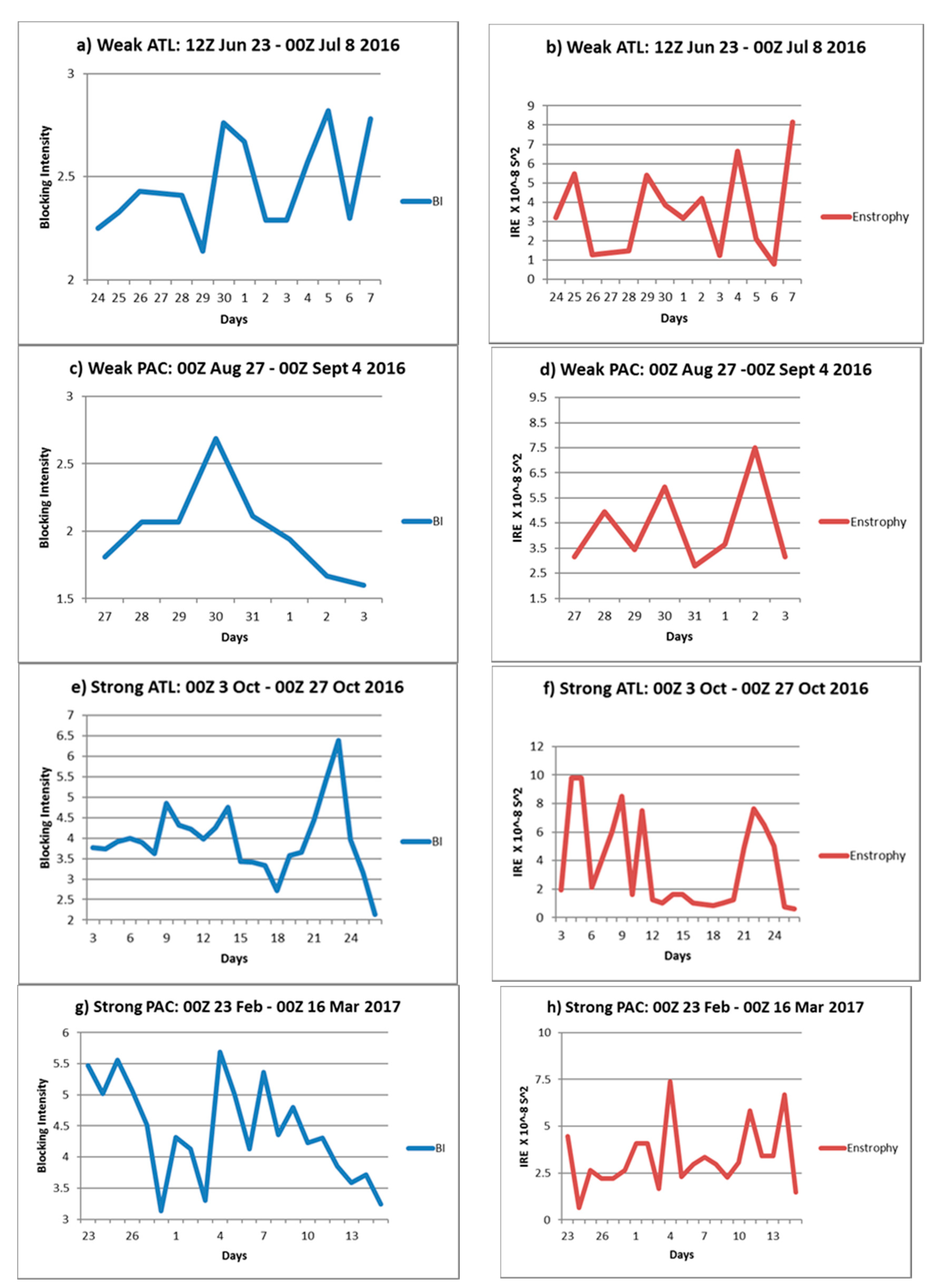
3. Synoptic Discussion and IRE

3.1. Weak Atlantic Event

This blocking event (Figure 1A) was located over the Atlantic Region and persisted for 14.5 days, as the onset was 1200 UTC 23 June 2016 and termination on 0000 UTC 8 July 2016 (Table 2). The BI was 2.42 (Table 2) ranking as moderate event, but closer to the weak classification [20]. The event was close to what is considered a typical intensity for an Atlantic Region warm season block [20], but a little stronger than the hemispheric mean. The center location of this weaker event drifted to the east and it’s termination occurred in the Ural Mountain region near 70° N. The BI (Figure 2a) remained relatively steady over the block life cycle ranging from 2.14 to 2.82, but going through four periods of increase and decrease in association with synoptic-scale cyclones (e.g., [6,31]). The IRE (Figure 2a) also increases during the onset phase and behaves in a similar manner to BI throughout the block lifecycle. The correlation between the two quantities (

Table 3. Correlation of IRE and BI for each event and for a lag of BI to IRE by 24-h increments out to 72-h. WA: Weak Atlantic, WP: Weak Pacific, SA: Strong Atlantic, PS: Pacific Strong, AW: Atlantic Weak, * best correlation, and ⁺, ⁺⁺, and ⁺⁺⁺ is correlation significant at least at the 90%, 95%, and 99% confidence level, respectively.

Correlation with Lag of BI
	Not Lagged	24-h	48-h	72-h
WA	0.29	0.40 *,+	−0.15	0.20
WP	0.15	−0.39	0.41 *	−0.26
SA	0.49 *,+++	0.40 ++	0.07	−0.20
SP	0.16	−0.31	−0.18	0.36 *,+

) was 0.29, which was not statistically significant.

3.2. Weak Pacific Event

The first Pacific Region blocking event examined here persisted for 8.0 days (Figure 1b), with onset at 0000 UTC 27 August 2016 and terminating on 0000 UTC 4 September 2016 (Table 2). This event was also considered a weak warm season event and the BI was 1.99 (Table 2), which is typical for blocking events that occur over the Pacific Region and the northern hemisphere during the warm season. The study of [20] found that cold season and oceanic region blocks were stronger in their research compared to warm season or continental blocking events. This event was nearly stationary in the zonal direction, but drifted slowly poleward within the western Pacific throughout the lifecycle. The intensity of the block (Figure 2c) changed some as well but was similar in strength at the beginning and end. At onset the block was weak with BI at 1.81 and continued to increase to a maximum BI of 2.69 in the middle of its lifecycle on 31 August 2016, and thereafter decreasing to 1.60 at termination. During the block lifecycle, the IRE (Figure 2d) was shown also to be steady and the correlation between BI and IRE was 0.15 (Table 3).

3.3. Strong Atlantic Event

During October 2016, a strong blocking event (Figure 1c) dominated the eastern Atlantic Region for 24 days, with the onset on 0000 UTC 3 October 2016 and terminating on 0000 UTC 27 October 2016 (Table 2). The BI was 3.96 (Table 2), which is a strong moderate event typical for an Atlantic, or northern hemisphere event during the fall or winter season [20]. This event, like the weak Atlantic blocking event discussed earlier drifted eastward and slightly poleward over the course of the lifecycle and terminating near the Urals. The BI diagnostic showed similar behavior to the previously discussed events, ranging from a BI of 2.72 on 18 October to a maximum BI of 6.38 on 23 October. The event was alternately moderate and strong over the lifecycle. The IRE behaved similarly to the BI and in this case the correlation between the two time series was 0.49 a value significant at the 99% confidence level. Additionally, the IRE does show a maximum at onset and towards decay suggesting flow regime transformation [27,28].

3.4. Strong Pacific Event

The strong Pacific blocking event (Figure 1d) was first identified on 0000 UTC 23 February 2017 near 50° N 160° W within the Bering Sea region in the eastern Pacific (Table 2). The event persisted for 21 days and remained relatively stationary before decay and the event terminated near the dateline on 0000 UTC 16 March 2017 (Table 2). The block was ranked as strong event with a BI of 4.40 (Table 2) making this event the strongest one examined here. On 4 March 2017, a second event deve-loped over the Atlantic region, which means that the Northern Hemisphere experienced simultaneous blocking (not shown). The Atlantic event was also strong and the observation that both events occurring simultaneously being strong was shown by [20]. The BI for the Pacific block ranged between 5.69 on 4 March 2017 and 3.13 on 28 February 2017 (Figure 2g). The mid-lifecycle peak was associated with strong upstream cyclone development and the onset of the Atlantic event. BI then decreased steadily until termination. The IRE was steady throughout the block lifecycle (Figure 2h), but peaked at the same time that BI was a maximum. The correlation between these two variables was about 0.16 (Table 3) which was not the highest among the samples studied, and this correlation is not statistically significant.

3.5. Discussion

The study of [3] and subsequent papers showed that the onset of every blocking event studied is accompanied by a developing surface cyclone and upper air short wave upstream of a large-scale ridge. They also noted the intensification of an upper-level jet maximum on the upstream flank of the blocking event, which strengthened the transport of anticyclonic vorticity into the developing blocking event. Then [6] demonstrated that the ideal phase relationship between the upstream low and developing blocking event is about 10°–50° longitude upstream. Each event studied here involved the same development mechanism and an example is shown in Figure 3.

At 1200 UTC 25 August (Figure 3a) as surface low is located near Manchuria and Sakhalin Island (52.5° N 140° E) with a central pressure of about 990 hPa. At this time, the surface low began rapid (but not explosive) development over the next 24-h and by 1200 UTC 26 August (Figure 3d) had a central pressure of 973 hPa. This represents a 17 hPa drop over 24 h, which is not quite the explosive development rate as defined by [32] for this latitude. Examining the wind field (Figure 3b,c) implies that the cyclone is located in the poleward exit region of a jet maximum located in the base of the upper-air trough at this time. Over that same 24 h, the wind maximum on the upstream flank of the block strengthens considerably as evidenced by the increases in u (Figure 3b,e,h) and v (Figure 3c,f,i) wind components. Figure 2d demonstrates that IRE increased during the early part of the block lifecycle along with the BI (Figure 2c). Thus, the peak in both variables occurs following the period of rapid upstream cyclone deepening.

The IRE peaks may be associated with peaks in the synoptic-scale component of the height field as shown by [7] for the July 2010 blocking event, which occurred over Russia. These peaks are likely associated with the deepening synoptic scale cyclone. Then it might be expected that the BI maxima may occur near the time of the IRE maxima as in [33]. However, a question that might be asked is whether the peak in IRE leads or lags peaks in BI or do they peak together?

To test this proposal correlation was performed with and without a time lag of each variable up to 72 h as in [34]. There were no positive correlations when BI led IRE. However, higher positive correlations were achieved for each event if the time series were lagged by up to 72 h such that IRE leads BI, or peaks in IRE occur first, then peaks in BI occurred. Table 3 shows that for three of the four events, the highest lag-correlation occurred 24, 48, or 72 h out. Only for the Strong Atlantic event did the peaks occur together. Also, for all the longer-lived events (all but the Weak Pacific event), the highest lag-correlations were significant at the 90% confidence level or greater. Lagging the time series such that BI lags IRE produces higher correlations as in [34]. Thus, we can modify the block onset paradigm of [3] by stating that first upstream cyclone deepening occurs, and then maxima in IRE will occur at or following block onset, with a maximum in BI at or following these events.

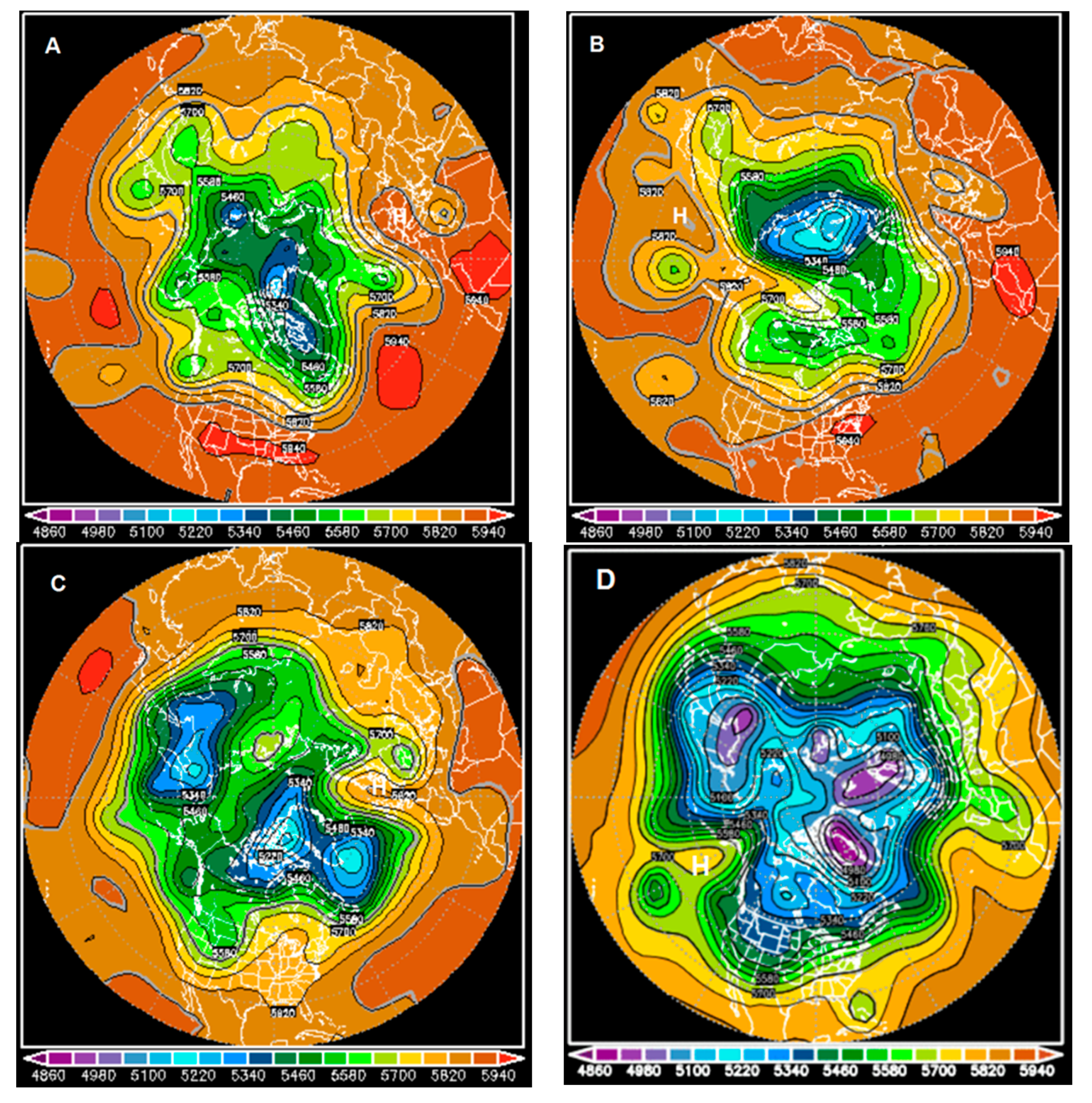
4. Ensemble Comparison

In order to examine the ability of the NCEP GEFS Ensemble to capture block onset and the intensity of these events, a comparison was made beginning with a seven-day lead time and going to the observed onset time. As stated above in Section 2.2, the ensemble mean was used since this produced the best comparison as shown in [27]. In order to summarize the results the focus was on seven-day, four-day, and one-day forecasts out to 240 h (10 days). The forecast blocking intensity was compared to the observed blocking intensity for only the days that the forecast showed blocking.

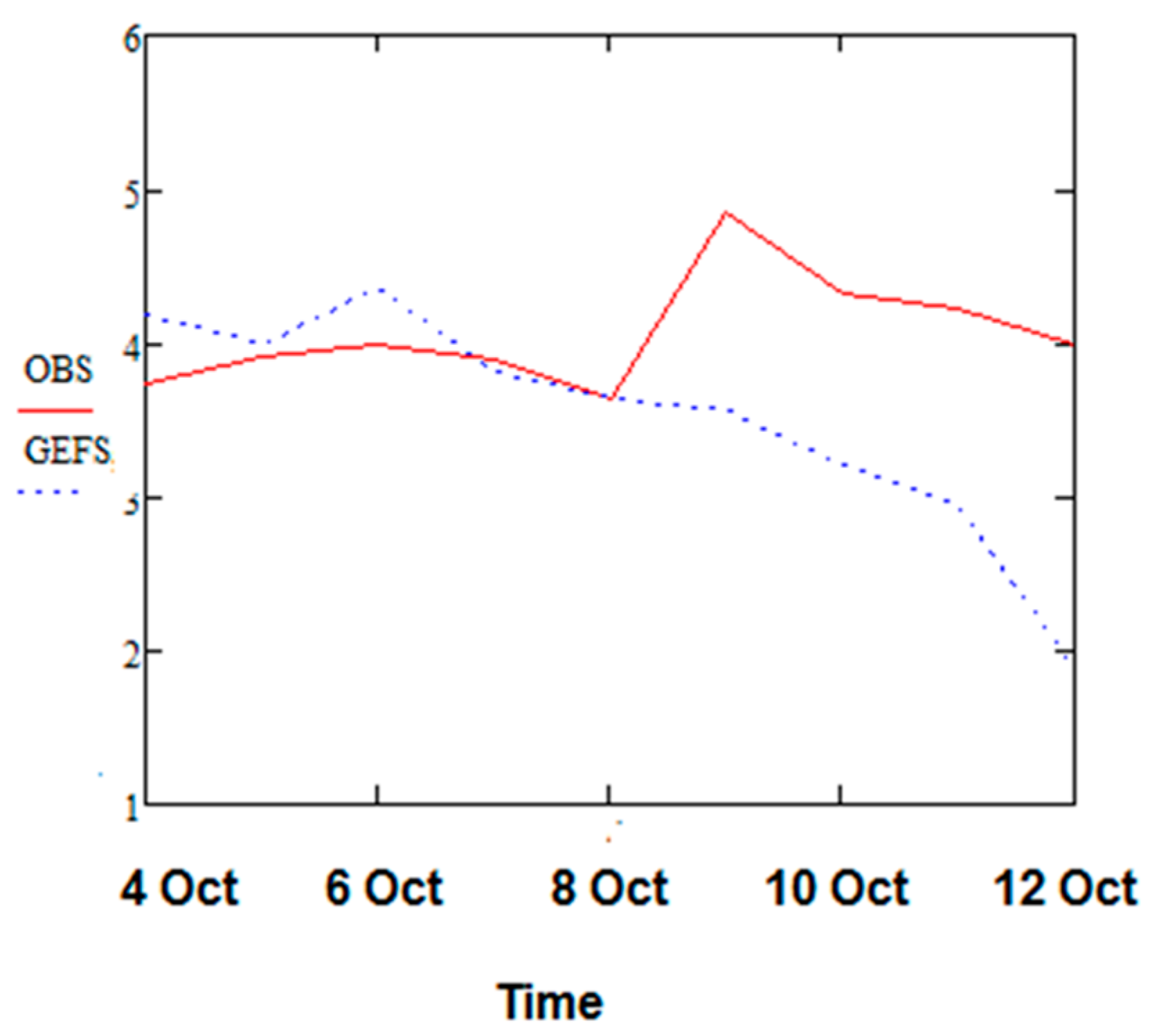
4.1. Seven-Day Forecasts

In examining the seven-day forecasts for all three events (

Table 4. The comparison in blocking intensity of the ensemble model forecast vs. observed blocking event during the validation period of all seven-day, four-day and one-day forecast for all four blocking events. N/A: no block present. The difference is OBS—MODEL. Dates of comparison are shown below the BI.

BI Comparison
Forecast/Blocks	Model BI	Observed BI	Difference
7 day
Block 1: WA	1.13	2.32	1.19
00Z 16 June 2016	(00/23–00/26)	(12/23–12/26)
Block 2: WP	1.74	2.69	0.95
00Z 20 August 2016	(00/30)	(12/30)
Block 3: SA	N/A	N/A	N/A
00Z 26 September 2016
Block 4: SP	N/A	N/A	N/A
00Z 16 February 2017
4 day
Block 1: WA	1.38	2.43	1.05
00Z 19 June 2016	(00/23–00/27)	(12/23–12/27)
Block 2: WP	1.82	2.18	0.36
00Z 23 August 2016	(00/28–00/1)	(12/28–12/1)
Block 3: SA	2.38	3.87	1.49
00Z 29 September 2016	(00/5–00/9)	(12/5–12/9)
Block 4: SP	3.12	4.93	1.71
00Z 19 February 2017	(00/23–0/28)	(12/23–12/28)
1 day
Block 1: WA	1.49	2.45	0.96
00Z 22 Jun 2016	(00/23–00/2)	(12/23–12/2)
Block 2: WP	1.73	2.05	0.32
00Z 28 August 2016	(00/27–00/2)	(00/27–00/2)
Block 3: SA	3.51	4.06	0.55
00Z 02 October 2016	(00/4-00/12)	(12/4–12/12)
Block 4: SP	4.47	4.93	0.46
00Z 22 February 2017	(00/23–0/28)	(12/23–12/28)

), only the summer season Weak Atlantic event was anticipated in any meaningful manner. The onset of this event was forecast well for the entire seven-day period before the observed onset (Table 4), however, the location of onset was 10 degrees longitude to the east (not shown). The GEFS model Weak Atlantic blocking event was forecast for the final four days of the period, but the BI was under-forecast by more than 50%, a difference of 1.19 BI units. For the Weak Pacific event, a strong ridge was placed in the right location (160° E) by the GEFS model and a block was identified for one day at the end of the 10-day forecast period and three days following the observed onset. Also, the BI for this one day in the GEFS was significantly lower than that of the observed event (Table 4—0.95 BI). For the other two cases, while no block was generated in the GEFS model, strong large-scale ridging was located near the observed block onsets.

In order to put the weak blocking event values into context, the work of [35] showed that surface sensible heating contributed 0.2–0.9 BI units to two southern hemisphere blocking events. Alternatively, as in [20], who examined the difference between the numerator and denominator in the BI calculation showed that a 50 m larger or smaller difference between the two values could produce a BI that is about 1.0 units larger or smaller, respectively. In the former case, this implies stronger upstream and downstream gradients, while in the latter case these gradients are weaker. Thus, this implies that the GEFS model blocking region gradients are weaker than observed by about 50 m seven days out.

4.2. Four-Day Forecasts

For each of the blocking events, the four-day GEFS mean ensemble model forecasts were similar in many respects. In each case, the block did develop at or within 10 degrees of the observed onset. Also, each case persisted for five or six days in the GEFS 10-day forecast period (Table 4), but did not exist as a blocking event by the 240 h time-period. Additionally, the intensity of each GEFS event was under-forecast, although the degree of under-forecasting BI varied considerably from 0.36 BI units in the case of the Weak Pacific Event to 1.71 BI units for the Strong Pacific event (Table 4). In each case, the GEFS blocking event BI was similar to the observed BI for the first two days, but by the end of forecast, the model BI diminished greatly and was under-forecast in some cases by more than two BI units.

Only the timing of the GEFS block onsets showed some variance from the observed (Table 4). For the Weak Atlantic and Strong Pacific events, the GEFS onset time occurred on the same day as the observed event. For the Weak Pacific event the GEFS block onset was 24 h later, while for the strong Atlantic Event the GEFS block onset was 48 h later than observed.

4.3. One-Day Forecasts

By the one-day forecast period, each of the GEFS mean ensemble blocking events were forecast well in terms of the timing of the onset (Table 4), and the location of onset was at the locations of the observed onset shown in Table 2. Only the Strong Atlantic event onset was 24 h later in the GEFS model than observed (Table 4), although since the GEFS ensembles were examined in 24 h increments the actual difference may be only 12 h. Also, there was some improvement in the GEFS forecast BI for the two weak events when compared to the four-day forecasts, however, for the two strong events the improvement was more dramatic.

Figure 4 shows the GEFS model blocking events at a similar time (12 h earlier) to the blocking events in Figure 2. The GEFS model events look very similar to the observed events, and given that these events are 48 h forecasts and close to the onset time, the model BI values are close to the observed values at this time. The model BI are given in Figure 4, and for the Weak Atlantic, Weak Pacific, and Strong Pacific events, the observed events are still stronger by 0.35, 0.25, and 0.37 BI units, respectively. For the Strong Atlantic event, the GEFS model event was stronger by 0.46 BI units. All of these values are within the BI values given by [35] for the contribution due to surface diabatic heating, or smaller than the 50 m difference between the numerator and denominator of BI given by [20].

4.4. Discussion

Overall, the NCEP GEFS mean ensemble forecasts were good for forecasting the location of the large-scale ridging and the onset of blocking. For the GEFS forecasts seven days out, the timing of block onset was only forecast well in one case (Weak Atlantic) and not even forecast for the two strong events. The two strong events were cold season events. By the four-day GEFS forecast period, all four events were forecast even if the onset time was late in two cases (weak Pacific and Strong Atlantic). At four days, however, all the blocking events were terminated by the GEFS model before the end of the 240 h forecast period even though all the observed events would have persisted beyond the 10 day forecast range. Even at one day, the timing of block onset in the GEFS model mean ensemble was missed by 24 h or less in one case (Strong Atlantic). For two of the events at this time, the GEFS model forecast the event to persist for the entire period which was observed (Weak Atlantic and Strong Atlantic). However, for the Strong Pacific event, the GEFS model did not show a block at the end of the 240 h period even though one was observed over the Pacific Region. However, during the 1–3 March period, the observed blocking event was transitioning during interaction with an upstream synoptic event. Also, for the Weak Pacific event, the termination of the block in the GEFS occurred 48 h before the decay of the observed event. Thus, the GEFS ensemble seemed to have more difficulty forecasting the persistence of Pacific Region blocking.

When examining the intensity of the GEFS blocking event and comparing these to the observed intensities, the GEFS model blocking events were weaker across all events, although the model forecast BI was improved as the initial forecast time approached the observed onset time. While it is not true that GEFS model block intensities were uniformly weaker across all time periods, the best comparison of model to observed BIs happened closest to onset (and the initialization period). An example of this behavior is shown in Figure 5. The GEFS model and observed blocking BI are similar for the first few days of the event, and for two of these days the model blocking was actually stronger. However, after 8 October 2016, the GEFS model BI decreased rapidly up to 12 October, while the observed events were relatively constant throughout the period.

Thus, the main findings in this section is that a GEFS mean ensemble model can forecast block onset reasonably at four days out, the models have difficulty with the persistence of the blocking event even with a one-day forecast in the Pacific Region. Also, the intensities are forecast better as the GEFS model initial time gets closer to observed onset, however, the model had difficulty in all instances of maintaining BI.

5. Summary and Conclusions

Four observed blocking events were studied here, two in the Atlantic and two and the Pacific Region and distributed among warm and cold season events as well as blocking events of different intensities. Using the NCEP/NCAR reanalysis data set as well as the NCEP GEFS model ensemble mean forecasts for a 240 h period, the ability of the model to forecast blocking intensity (BI), longevity, onset, decay, and location. Here we used the 500-hPa heights and the [20] criterion to identify blocking and calculate intensity. Additionally, the IRE was calculated and compared to the BI following [34].

• Overall in all cases location, the GEFS model best captured decay and longevity while blocking intensity and onset were underestimated, BI showing the worst performance;
• IRE was introduced to determine if there could be a relationship between this quantity and BI. Here it was found that there was a lag relationship between IRE and BI by up to 72 h as indicated by statistically significant correlations between the two time series. This result is consistent with the results of [31,34]. In the future, in order to expand on this work it is possible to introduce the [14] probabilistic forecast to increase accuracy in blocking intensity and onset;
• The GEFS mean ensemble model performed the worst in capturing BI, although this was not the case uniformly across all time-periods. The model had difficulty maintaining BI in all events and forecast time periods;
• The persistence of blocking was forecast better for the Atlantic Region events than for the Pacific Region events.

References

1. Shukla, J.J.; Mo, K.C. Seasonal and Geographical Variation of Blocking. Mon. Weather Rev. 1983, 111, 388–402. [Google Scholar] [CrossRef]
2. Lejenas, H.; Okland, H. Characteristics of Northern Hemisphere blocking as determined from a long time series of observational data. Tellus 1983, 35, 350–362. [Google Scholar] [CrossRef]
3. Lupo, A.R.; Smith, P.J. Climatological features of blocking anticyclones in the Northern Hemisphere. Tellus 1995, 47, 439–456. [Google Scholar] [CrossRef]
4. Matsueda, M.; Kyouda, M.; Toth, Z.; Tanaka, H.L.; Tsuyuki, T. Predictability of an Atmospheric Blocking Event that Occurred on 15 December 2005. Mon. Weather Rev. 2011, 139, 2455–2470. [Google Scholar] [CrossRef]
5. Lupo, A.R.; Smith, P.J. Planetary and Synoptic-Scale Interactions during the Life Cycle of a Mid-Latitude Blocking Anticyclone over the North Atlantic. Tellus Spec. Issue Life Cycles Extratrop. Cyclones 1995, 47, 575–596. [Google Scholar]
6. Lupo, A.R.; Bosart, L.F. An Analysis of a Relatively Rare Case of Continental Blocking. Quart. J. R. Meteorol. Soc. 1999, 125, 107–138. [Google Scholar] [CrossRef]
7. Lupo, A.R.; Mokhov, I.I.; Akperov, M.G.; Cherokulsky, A.V.; Athar, H. A dynamic analysis of the role of the planetary and synoptic scale in the summer of 2010 blocking episodes over the European part of Russia. Adv. Meteorol. 2012, 584257. [Google Scholar] [CrossRef]
8. Lorenz, E.N. Deterministic Nonperiodic Flow. J. Atmos. Sci. 1963, 20, 130–141. [Google Scholar] [CrossRef]
9. Lorenz, E.N. A study of the predictability of a 28-variable model. J. Atmos. Sci. 1965, 20, 130–141. [Google Scholar] [CrossRef]
10. Lupo, A.R.; Li, Y.C.; Feng, Z.C.; Fox, N.I.; Rabinowitz, J.L.; Simpson, M.A. Sensitive Versus Rough Dependence in Initial Conditions in Atmospheric Flow Regimes. Atmosphere 2016, 7, 157. [Google Scholar] [CrossRef]
11. Tibaldi, S.S.; Tosi, E.E.; Navarra, A.A.; Pedulli, L.L. Northern and Southern Hemisphere Seasonal Variability of Blocking Frequency and Predictability. Mon. Weather Rev. 1994, 122, 1971–2003. [Google Scholar] [CrossRef]
12. Colucci, S.J.; Baumhefner, D.P. Numerical Prediction of the Onset of Blocking: A Case Study with Forecast Ensembles. Mon. Weather Rev. 1998, 126, 773–784. [Google Scholar] [CrossRef]
13. Colucci, S.J.; Alberta, T.L. Plaetary-scale climatology of explosive cyclogenesis and blocking. Mon. Weather Rev. 1996, 124, 2509–2520. [Google Scholar] [CrossRef]
14. Watson, J.S.; Colucci, S.J. Evaluation of Ensemble Predictions of Blocking in the NCEP Global Spectral Model. Mon. Weather Rev. 2002, 130, 3008–3021. [Google Scholar] [CrossRef]
15. Brankovic, C.; Palmer, T.N.; Molteni, F.; Tibaldi, S.; Cubasch, U. Extended-range predictions with ECMWF models: Time-lagged ensemble forecasting. Quart. J. R. Meteorol. Soc. 1990, 116, 857–912. [Google Scholar] [CrossRef]
16. Wilks, D.S. Statistical Methods in the Atmospheric Sciences: An Introduction; Academic Press: New York, NY, USA, 1995; p. 467. [Google Scholar]
17. Jensen, A.D.; Lupo, A.R. Using Enstrophy Advection as a Diagnostic to Identify Blocking Regime Transition. Quart. J. R. Meteorol. Soc. 2013, 139, 2–7. [Google Scholar] [CrossRef]
18. Dymnikov, V.P.; Kazantsev, Y.V.; Kharin, V.V. Information entropy and local Lyapunov exponents of barotropic atmospheric circulation. Izv. Atmos. Ocean. Phys. 1992, 28, 425–432. [Google Scholar]
19. Toth, Z.; Kalnay, E. Ensemble Forecasting at NMC: The Generation of Perturbations. Bull. Am. Meteorol. Soc. 1993, 74, 2317–2330. [Google Scholar] [CrossRef]
20. Wiedenmann, J.M.; Lupo, A.R.; Mokhov, I.I.; Tikhonova, E.A. The Climatology of Blocking Anticyclones for the Northern and Southern Hemispheres: Block Intensity as a Diagnostic. J. Clim. 2002, 15, 3459–3473. [Google Scholar] [CrossRef]
21. Tracton, M.; Kalnay, E. Operational Ensemble Prediction at the National Meteorological Center: Practical Aspects. Weather Forecast. 1993, 8, 379–398. [Google Scholar] [CrossRef]
22. National Center for Environmental Prediction/Natioanl Center for Atmospheric Research Reanalysies. Available online: https://www.esrl.noaa.gov/psd/data/reanalysis/reanalysis.shtml (accessed on 20 June 2017).
23. Kalnay, E.E.; Kanamitsu, M.M.; Kistler, R.; Collins, W.; Deaven, D.; Gandin, L.; Iredell, M.; Saha, A.; White, G.; Woollen, J.; et al. The NCEP/NCAR 40-Year Reanalysis Project. Bull. Am. Meteorol. Soc. 1996, 77, 437–471. [Google Scholar] [CrossRef]
24. Rex, D.F. Blocking action in the middle troposphere and its effect on regional climate II: The climatology of blocking action. Tellus 1950, 3, 275–301. [Google Scholar]
25. Triedl, R.A.; Birch, E.C.; Sajecki, P. Blocking action in the Northern Hemisphere: A climatological study. Atmos. Ocean 1981, 19, 1–23. [Google Scholar] [CrossRef]
26. Shapiro, R. Smoothing, filtering, and boundary effects. Rev. Geophys. 1970, 8, 359–387. [Google Scholar] [CrossRef]
27. Jensen, A.D.; Lupo, A.R. Using Enstrophy Based Diagnostics in an Ensemble for Two Blocking Events. Adv. Meteorol. 2013, 2013, 693859. [Google Scholar] [CrossRef]
28. Jensen, A.D.; Lupo, A.R. The Role of Deformation and Other Quantities in an Equation for Enstrophy as Applied to Atmospheric Blocking. Dyn. Atmos. Oceans 2014. [Google Scholar] [CrossRef]
29. Lupo, A.R.; Mokhov, I.I.; Dostoglou, S.; Kunz, A.R.; Burkhardt, J.P. The impact of the planetary scale on the decay of blocking and the use of phase diagrams and enstrophy as a diagnostic. Izv. Atmos.-Ocean 2007, 43, 45–51. [Google Scholar] [CrossRef]
30. Universiy of Missouri Blocking Archive. Available online: http://weather.missouri.edu/gcc (accessed on 21 June 2017).
31. Lupo, A.R. A Diagnosis of Two Blocking Events That Occurred Simultaneously in the Midlatitude Northern Hemisphere. Mon. Weather Rev. 1997, 125, 1801–1823. [Google Scholar] [CrossRef]
32. Sanders, F.; Gyakum, J.R. Synoptic-dynamic climatology of the “bomb”. Mon. Weather Rev. 1980, 108, 1577–1589. [Google Scholar] [CrossRef]
33. Jensen, A.D. A dynamic analysis of a record breaking winter season blocking event. Adv. Meteorol. 2015, 2015, 634896. [Google Scholar] [CrossRef]
34. Jensen, A.D.; Lupo, A.R.; Mokhov, I.I.; Akperov, M.G. Integrated Regional Enstropy and Block Intensity as a Measure of Kolmogorov Entropy. Atmosphere 2017. submitted. [Google Scholar] [CrossRef]
35. Tilly, D.E.; Lupo, A.R.; Melick, C.J.; Market, P.S. Calculated height tendencies in a Southern Hemisphere blocking and cyclone event: The contribution of diabatic heating to block intensification. Mon. Weather Rev. 2008, 136, 3568–3578. [Google Scholar] [CrossRef]
Figure 1. The 500 hPa height field for (A) 1200 UTC 24 June 2016 (weak Atlantic); (B) 1200 UTC 28 August 2016 (weak Pacific); (C) 1200 UTC 4 October 2016; and (D) 1200 UTC 24 February 2017. The center point at this time is labelled with an ‘H’.
Proceedings 01 00087 g001
Figure 2. The (a,c,e,g) BI (no units) and (b,d,f,h) IRE (× 10−8 s−2) for the weak Atlantic, weak Pacific, strong Atlantic, and strong Pacific blocking events, respectively.
Proceedings 01 00087 g002
Figure 3. The (a,d,g) sea level pressure (Pa) (left column), (b,e,h) u-wind component (m s−1) (middle column), and (c,f,i) v-wind component (m s−1) (right column) for 1200 UTC 25 August (top row), 1200 UTC 26 August (middle row), and 1200 UTC 27 August 2016 (bottom row), respectively.
Proceedings 01 00087 g003
Figure 4. As in Figure 2 for the GEFS 48 h forecast, except for 12 h earlier. The block center is identified with a white ‘H’. BI for each event is (A) 1.98; (B) 1.82; (C) 4.19; and (D) 4.75.
Proceedings 01 00087 g004
Figure 5. The Strong Atlantic blocking event observed BI (red—solid) and GEFS model BI (blue dotted) for the one-day GEFS ensemble mean forecast period.
Proceedings 01 00087 g005