Proceeding Paper

Sensitivity of Precipitation to Aerosol and Temperature Perturbation over the Foothills of the Nepal Himalayas †

by
Rudra K. Shrestha
1,2,*,
Paul J. Connolly
2 and
Martin W. Gallagher
2
1
Canadian Centre for Climate Modelling and Analysis (CCCma), Environment and Climate Change Canada (ECCC), Victoria, British Columbia V8P 5C2, Canada
2
Center for Atmospheric Science, School of Earth, Atmospheric and Environmental Sciences, The University of Manchester, Oxford Road, Manchester M13 9PL, UK
*
Author to whom correspondence should be addressed.
Presented at the 2nd International Electronic Conference on Atmospheric Sciences, 16–31 July 2017; Available online: http://sciforum.net/conference/ecas2017.
Proceedings 2017, 1(5), 144; https://doi.org/10.3390/ecas2017-04146
Published: 17 July 2017

Abstract

:
Increasing the amount of anthropogenic aerosols over the Himalayas modulate cloud properties, thereby altering cloud phase and cloud height, consequently influence formation and distribution of orographic precipitation. Moreover, further rises in global temperature may influence cloud properties by the ‘Clausius—Clapeyron effect’, which increases moisture holding capacity of air. This study presents sensitivity of simulated cloud properties to aerosol and temperature perturbations using the Weather Research and Forecasting (WRF) model, coupled with a bulk microphysics scheme, in a convection permitting configuration applied to a complex topographical region, the Nepal Himalayas. We find that the effect of aerosol on the simulated rainfall is nonlinear, ranging from −3% to +4% depending on the investigated aerosol perturbation scenarios. The model results highlight a realistic simulation of the 1st indirect (Twomey) effect. However, the rainfall was not overly sensitive to the aerosol perturbations and not statistically significant at the 95% confidence interval. The oversimplified parameterization of ice phase processes, a dominant cloud formation process over the Himalayas, appears to play a crucial role in buffering the sensitivity to increased aerosol loading. Our results, however, show that aerosol perturbations may modify shape, size and spatial distribution of individual cloud and their precipitation production. In contrast, the impact of temperature perturbations is more than the aerosol effect, ranging from −17% to +93%, which is statistically significant at the 95% confidence interval, suggesting that more intense rain events are likely as the climate warms in this region.

1. Introduction

The majority of the population in South Asia are dependent upon monsoon precipitation for their daily lives [1,2,3]. An accurate prediction of the monsoon onset and decay, its movement and variability is critical [4,5] which subsequently influences rainfall dependent agriculture [3] that provides security for the majority of the working population [6].
The impacts of global warming on the Indian monsoon precipitation are uncertain [7], which may be associated with uncertainties in the projections of future climate change [8]. An assessment of the Intergovernmental Panel on Climate Change (IPCC, 2014) shows that the annual mean surface temperature across the Tibetan Plateau region in the high greenhouse gas concentration scenario (RCP8.5), often thought of as a ‘worst case’, will produce a rise in ~9 °C by the end of 21st century. Furthermore, IPCC [9] emphasizes that the RCP2.6, considered as a very low greenhouse gas concentration scenario, predicts ~1.5 °C positive surface temperature anomaly across the region. Recent studies have highlighted that the Himalayan region is warming faster than the other parts of the world [10,11,12], which increase moisture holding capacity of air [13], known as the ‘Clausius—Clapeyron effect’. Consequently, the resulting enhanced water vapour in the atmosphere may increase potential for heavy precipitation in convective or orographic initiated storms due to additional latent heat release that invigorates the storm.
It is hypothesised that the monsoon precipitation is affected by the enhanced aerosol loadings in South Asia [14,15] as aerosols act as a source of additional cloud condensation nuclei (CCN). In warm stratus clouds, increased aerosols may subsequently decrease average cloud droplet effective radius altering cloud radiative forcing—the first indirect effect [16]. Smaller cloud droplets consequently suppress rainfall for a given water path—the second indirect effect for warm clouds and also increase their lifetime [17]. In addition to their contribution to CCN effects, anthropogenic aerosols are identified as one of the major sources of Ice Nuclei (IN) [18,19], and can influence several other ‘indirect effects’ such as ‘thermodynamic’, ‘glaciation’ and ‘riming’ which may modulate mixed-phase properties of clouds [20].
A complete understanding of the Indian monsoon system is complicated [2] owing to the role of the rugged topography of the Himalayas [21], its interactions with large scale dynamics, and cloud microphysics that cause wide ranging impact on pollution transport, cloud and precipitation [22]. Shrestha et al. [23] suggest that the advected aerosols from the Indo-Gangetic Plains is confined within the valleys, localizing their properties, which in turn play a critical role in modulating cloud microphysical and precipitation processes. This effect was observed in the Sierra Nevada Mountains, according to Lynn et al. [24], where ‘clean-air’ produce more and aged ‘dirty-air’ produce less precipitation in the foothills of the mountains. Furthermore, the pristine air mass across the Caliafornia Mountains produce 30% more precipitation than the aged polluted air [25]. An increasing aerosol number concentrations over the Swiss Alps (e.g., in the region of the Jungfraujoch Mountain) seemed to suppress warm cloud processes, leading to a decrease in orographic precipitation on the upslope of the mountains [26]. However, the relation between aerosols and precipitation is not always linear, which may depend on environmental conditions of the study area [24]. A non-linear relationship between aerosol and precipitation is observed in a tropical convective system, and also the precipitation amount is not overly sensitive to aerosol perturbations [27,28].
In this paper we aim to investigate how aerosol and temperature perturbations may affect cloud microphysical processes and to what extent subsequent aerosol—cloud interactions may alter precipitation formation and distribution over the complex terrain of the Himalayas. We address the following questions:
  • How will the precipitation respond to aerosol and temperature perturbations?
  • How is the spatial distribution of the precipitation affected by aerosol perturbations?
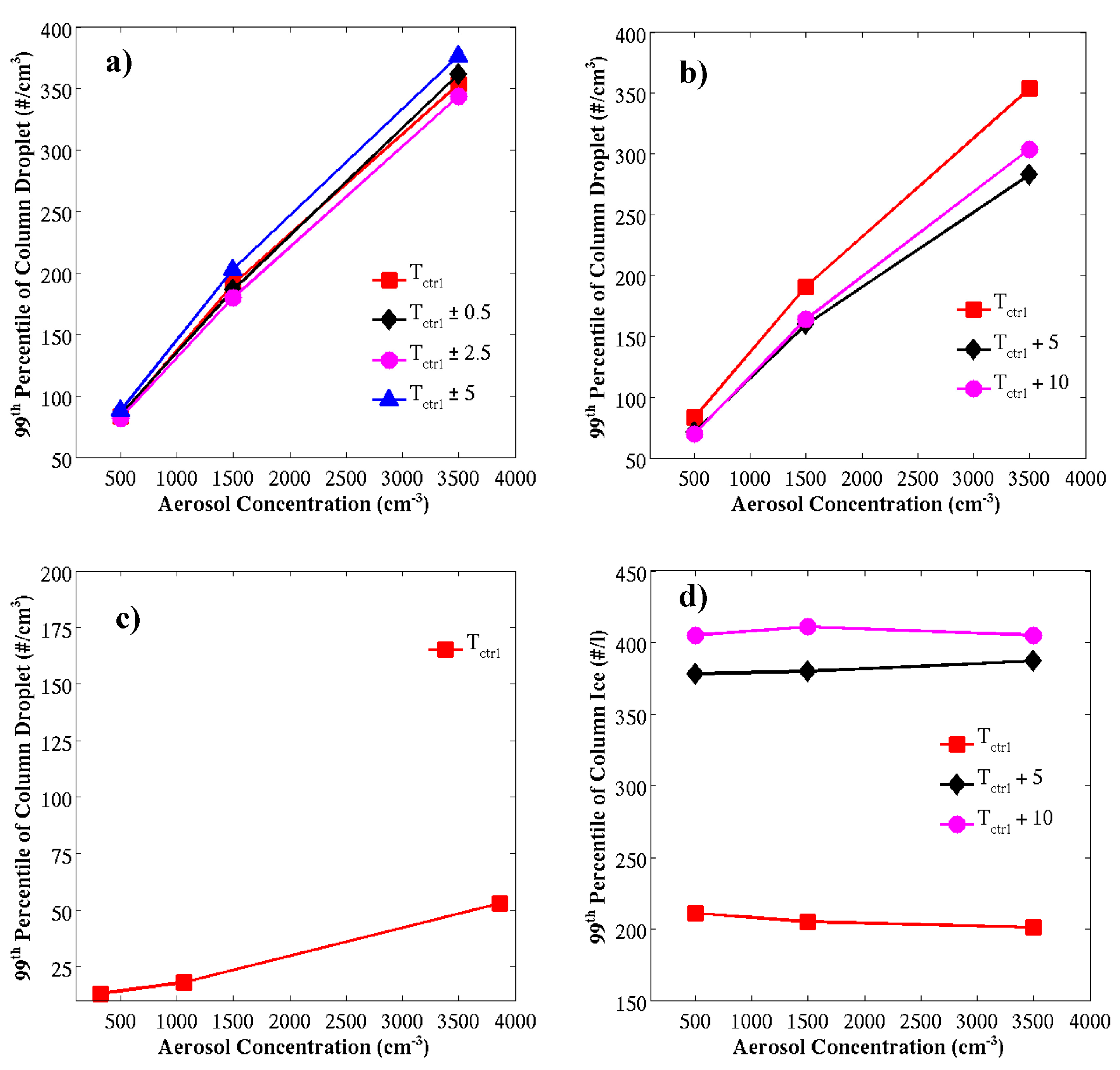
  • How are these perturbations manifested in the microphysical properties of the clouds?
This paper is organized as follows: the numerical model and microphysics are explained in Section 2 and Section 3 respectively; Section 4 outlines the experimental set up and the results follow in Section 5. A discussion and conclusion is presented in Section 6.

2. Numerical Model

The simulations described here were carried out using version 3.1.1 of the Weather Research and Forecasting (WRF) model. The model incorporates the advanced Research WRF (ARW) mass based, terrain following vertical coordinate system, with adjustable vertical grid spacing. Prognostic variables include vertical and horizontal wind components, microphysical quantities, perturbation potential temperature, geopotential and surface pressure of dry air. Twenty four categories from the USGS ‘30s’ global data set were used to initialize surface properties such as terrain, vegetation index and land use type.
The model uses a 3rd order Runge—Kutta time integration scheme with 5th order horizontal and 3rd order vertical momentum advection options. A gravity wave absorbing layer was used to damp anomalously large vertical velocities in the model [29]. A complete description of the WRF model is provided by Skamarock et al. [30].
The WRF model has been widely tested and successfully applied for the evolution of mesoscale weather phenomenon in areas of complex topography [31,32]. The studies by Ikeda et al. [33], Rasmussen et al. [34] and Liu et al. [35], show that orographic precipitation from simulations with the WRF model are comparable with observations in complex terrain. Furthermore, Maussion et al. [36] applied the WRF model to simulate a precipitation event over the Tibetan Plateau and compared with the Tropical Rainfall Measuring Mission (TRMM) satellite observations. The simulated precipitation was consistent with the satellite observation, giving confidence that our set-up will also be suitable for this study.

3. Cloud Microphysical Description
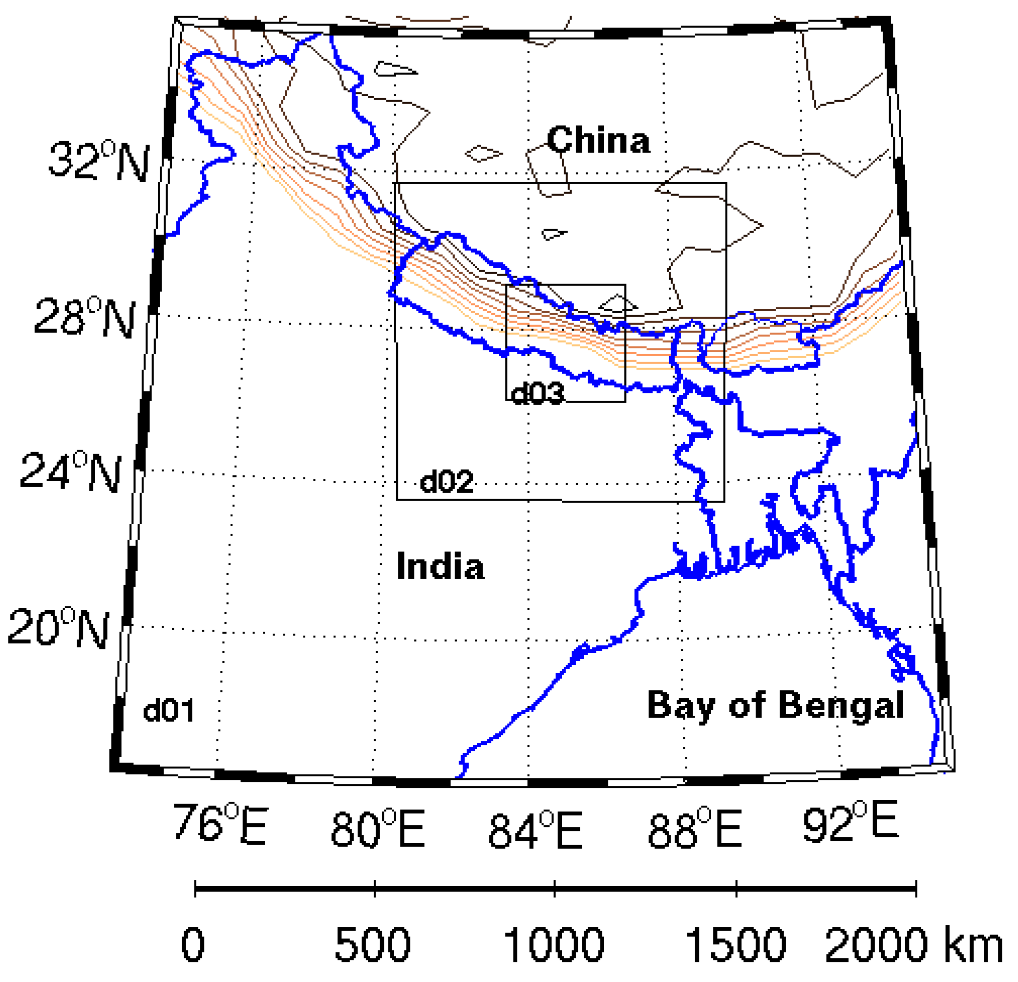
The Morrison double-moment bulk cloud microphysical scheme [37,38] was used in WRF in this study. This double moment microphysics scheme thus predicts the number concentration and the mixing ratio of different hydrometeors. Prognostic equations are used to describe the evolution of five hydrometeor species (cloud droplets, rain, cloud ice, snow and graupel) and water vapour. CCN activation is parameterized following the standard Twomey [39] power-law relation, Nc = Csk, using the modification described by Rogers and Yau [40] for use in this model. This scheme does not explicitly include calculation of peak super-saturation, since this is not resolved by the model grid, but instead it calculates the number of activated droplets as a function of updraft velocity. The maximum super-saturation is therefore implicit in this formulation, as it mainly depends on updraft speed and the CCN characteristics (C and k). Following Twomey [39], the equation governing the number of CCN activated at cloud base is:
N = 0.88 C 2 / ( k + 2 ) [ 7 × 10 2 × U 3 / 2 ] k / ( k + 2 )
where N describes the total number of activated droplets (cm−3). The vertical velocity, which includes grid and sub-grid scale velocity, is represented by U (cm s−1), C is the CCN number concentration (cm−3) at 1% supersaturation, and k represents an activation parameter that depends on air mass type and which may vary from 0.4 to 1.0. In this study we use a constant value of k equal to 0.8.
In Morrison scheme the warm rain process is parameterized using the method of Khairoutdinov and Kogan [41] which was arrived at by regression analysis against droplet size spectra predicted by an explicit bin-microphysical model. The ice phase descriptions in the model include diffusional growth, aggregation, riming and melting of ice hydrometeors (processes relevant for cloud ice crystals, snow and graupel). Heterogeneous ice nucleation was parameterized following Rasmussen et al. [42], where primary ice crystals are generated through immersion freezing, contact freezing and deposition and condensation nucleation. Ice multiplication processes were parameterized following Hallett and Mossop [43].

4. Model Setup

The model was configured using three (two-way) nested domains with a horizontal grid resolution of 27, 9 and 3 km centred over central Nepal (26.34° N, 83.12° E) defined in the Lambert conformal projection (Figure 1). The outermost domain (Domain 1) covered Asian monsoon region including the Himalayas, the Indian subcontinent and the Bay of Bengal to capture regional flow patterns. Domain 2 covered the entire Nepal region including the central Himalayas and part of Northern India in order to capture mesoscale circulation. The innermost high resolution domain (Domain 3) covers central Nepal focusing on circulation over the foothills and valleys of the Himalayas. Evaluation of the model results is focused on the high resolution (3 km × 3 km) domain which contains 111 × 111 horizontal grid points and 40 vertical levels with the domain top pressure of 50 mb. First few hours of the simulation is considered as a spin-up run and not included in the calculation. The model integration time-step was set to 30 s. We use NCEP/DOE reanalysis 2 data for model initialisation and boundary conditions. The physics packages include the Dudhia short-wave radiation [44], the RRTM long-wave radiation [45], the YSU boundary layer [46] and the Noah land surface models. No cumulus parameterization was used in the high resolution (3 km × 3 km) simulations presented here as the model set up should explicitly resolve the cumulus convection in sufficient detail, but the Grell-Devenyi ensemble scheme was used in the lower resolution domains.
The atmospheric moisture content was altered by perturbing the temperature (i) uniformly and (ii) randomly across the domain by modifying the model standard code and holding the relative humidity constant. In the uniform perturbation case a constant increment is added to the unperturbed (control) temperature (hereafter Tctrl) at every model grid point. Two different temperature enhancement scenarios (i) Tctrl + 5, and (ii) Tctrl + 10 were created with respect to the Tctrl run by adding ΔT = 5 °C and 10 °C, respectively. In contrast, the random perturbation was created using a random number generator. The range of perturbations was restricted to between ΔT = −0.5 °C to +0.5 °C, ΔT = −2.5 °C to +2.5 °C and ΔT = −5.0 °C to +5.0 °C, forming three different temperature perturbation scenarios relative to the control simulation, i.e., (i) Tctrl ± 0.5, (ii) Tctrl ± 2.5, and (iii) Tctrl ± 5. The aerosol concentrations were prescribed as 500 cm−3, 1500 cm−3 and 3500 cm−3 referred to as the ‘low’, ‘medium’ and ‘high’ aerosol cases, respectively. These aerosol perturbation scenarios provide only approximate ranges for the region [23], with the high aerosol case being considered as biomass burning event, for example. However these need to be verified with further observations.
We also used a more realistic approach to investigate aerosol perturbation effects on precipitation response by implementing a prognostic CCN scenario. For this we modified the standard WRF model code to predict CCN as a function of time and position within the domain. Aerosol number concentration remains constant from ground level to an altitude of 3500 m, followed by linear reduction in concentration up to 4000 m and then decreases logarithmically. We also used aerosol parameters that were derived from the Aerosol and Chemical Transport in Tropical Convection (ACTIVE) field campaign [47] to initialize the model, the study uses similar assumption for the ‘low’, ‘medium’ and ‘high’ aerosol scenarios as we did here.
To investigate the sensitivity of rainfall to aerosol and temperature perturbations we applied the range of initial conditions to three real rainfall events that occurred during different seasons of a one year period with varying rainfall intensity. This resulted in 45 WRF simulations in total. In the first case (Case I) the model was initialized at 00 UTC (11:45 Local) on 06 September 2007 and ran for 24 h. This case was characterized by monsoonal flow from the Bay of Bengal, and may be referred to as a moderate intensity rain case. The second case (Case II) was initialized at 12 UTC (17:45 Local) on 25 September 2011 and ran for 30 h. This case was strongly influenced by moist monsoonal flow and representative of a high intensity rain event. In the final (Case III) the model was initialized at 00 UTC on 27 March 2011 and ran for 24 h. This case is characteristic of a winter monsoon case influenced by extra-tropical cyclones, locally known as western disturbance, and was a low intensity rainfall event. In addition to the aerosol scenarios, the case-I was examined for the uniform temperature perturbation, random temperature perturbation and prognostic CCN scenarios, whereas the case studies II and III were investigated for the random temperature perturbation and the aerosol cases.

5. Results

We analyze the sensitivity of rainfall to aerosol and temperature perturbations using experimental and control run simulations. The domain averaged accumulated rain (hereafter accumulated rain), the domain and time averaged cloud droplet effective radius and ice crystal effective radius (hereafter Rc,eff and Ri,eff, respectively) are investigated. Furthermore, cloud droplet number concentration (hereafter CDNC) is also analyzed to examine the sensitivity of aerosol and temperature perturbations.

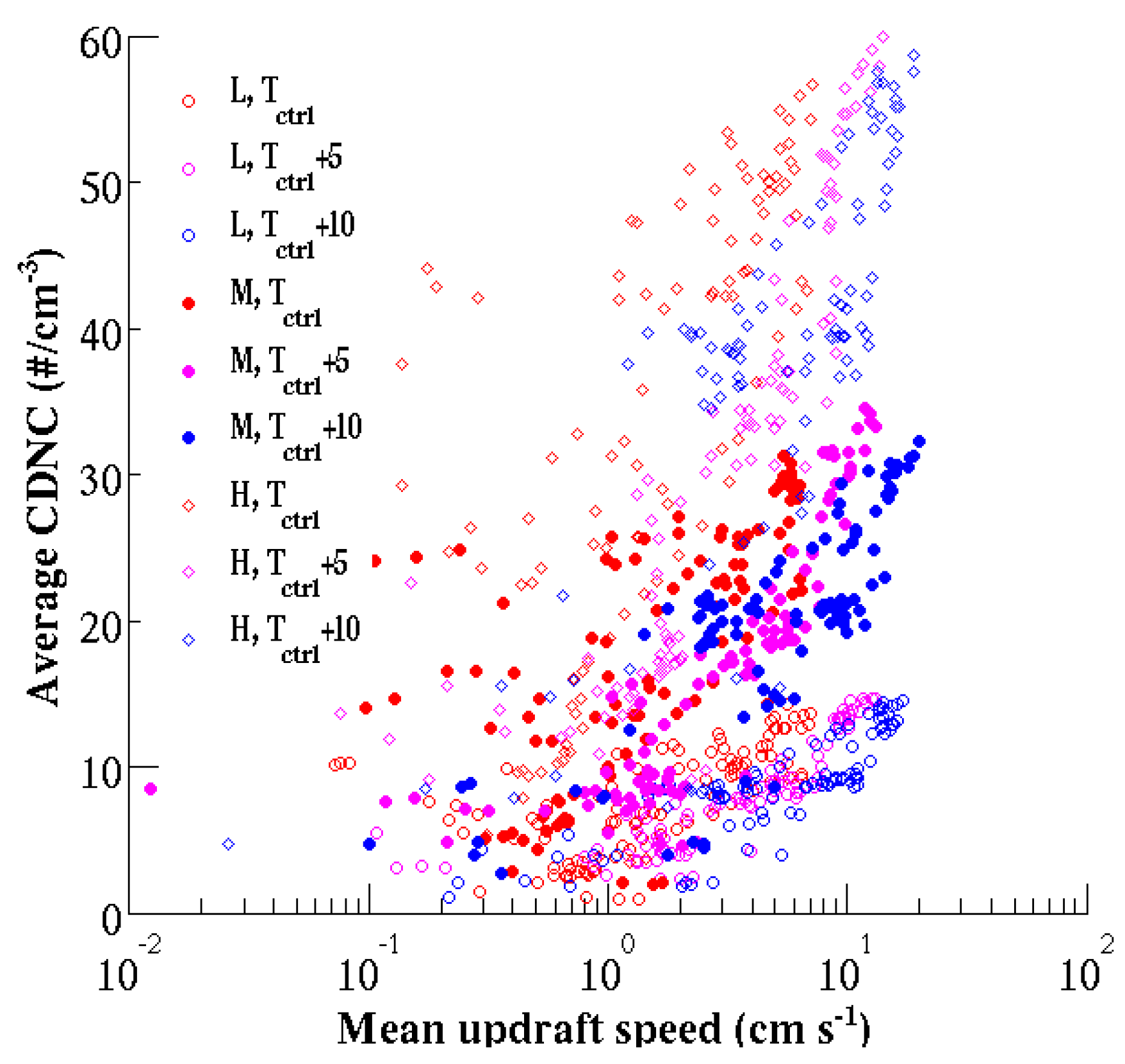
5.1. Activation of CCN and IN

5.1.1. Case Study I

As expected, the majority of our simulations show greater that aerosol concentrations give rise to clouds with smaller Rc,eff (Table 1) and greater droplet number concentrations (Nc) (Figure 2a–c). However, no consistent effects of the aerosol perturbations were observed on Ri,eff (Table 2) and ice number concentration (Ni) (Figure 2d). The effects of temperature perturbations on cloud droplet activation were not significant. However, they showed a strong positive effect on ice nucleation processes, producing more ice crystals concentrations with increasing temperature. A good correlation between positive vertical velocity (Wa), which play a role to activate aerosol particles, and corresponding CDNC was found (Figure 3).

5.1.2. Case Study II

Our results show that CDNC increases with increasing aerosol concentrations. The effect of temperature perturbations on droplet activation was not significant, even less effective than in the case I. Consistent with strong and organized updraft, relative to the other cases described in this study, a stronger positive correlation between CDNC and Wa was found. A decreased Rc,eff, consistent with the case I, was observed with an increase in aerosol concentration, however the effects of temperature was non-monotonic (Table 1). Our simulations indicate that aerosol perturbations exert minimal impact on Ri,eff. In contrast, the effect of temperature perturbations is significant and non-linear (Table 2).

5.1.3. Case Study III

Consistent with previous cases, a positive correlation was observed between CDNC and aerosol perturbations. As this is low rainfall event, the impact of temperature perturbations on droplet activation was negligible. Unlike the previous cases correlation between CDNC and Wa was not so strong in this case, as the event is characterized by weak updraft velocity, in turn, show limited numbers of activated droplets. Furthermore, as opposed to the previous cases, Rc,eff remained unchanged with increasing aerosol number concentration (Table 1) and also minimal impact was observed on Ri,eff. The impact of temperature perturbations on Rc,eff, and Ri,eff are shown in Table 1 and Table 2, respectively.

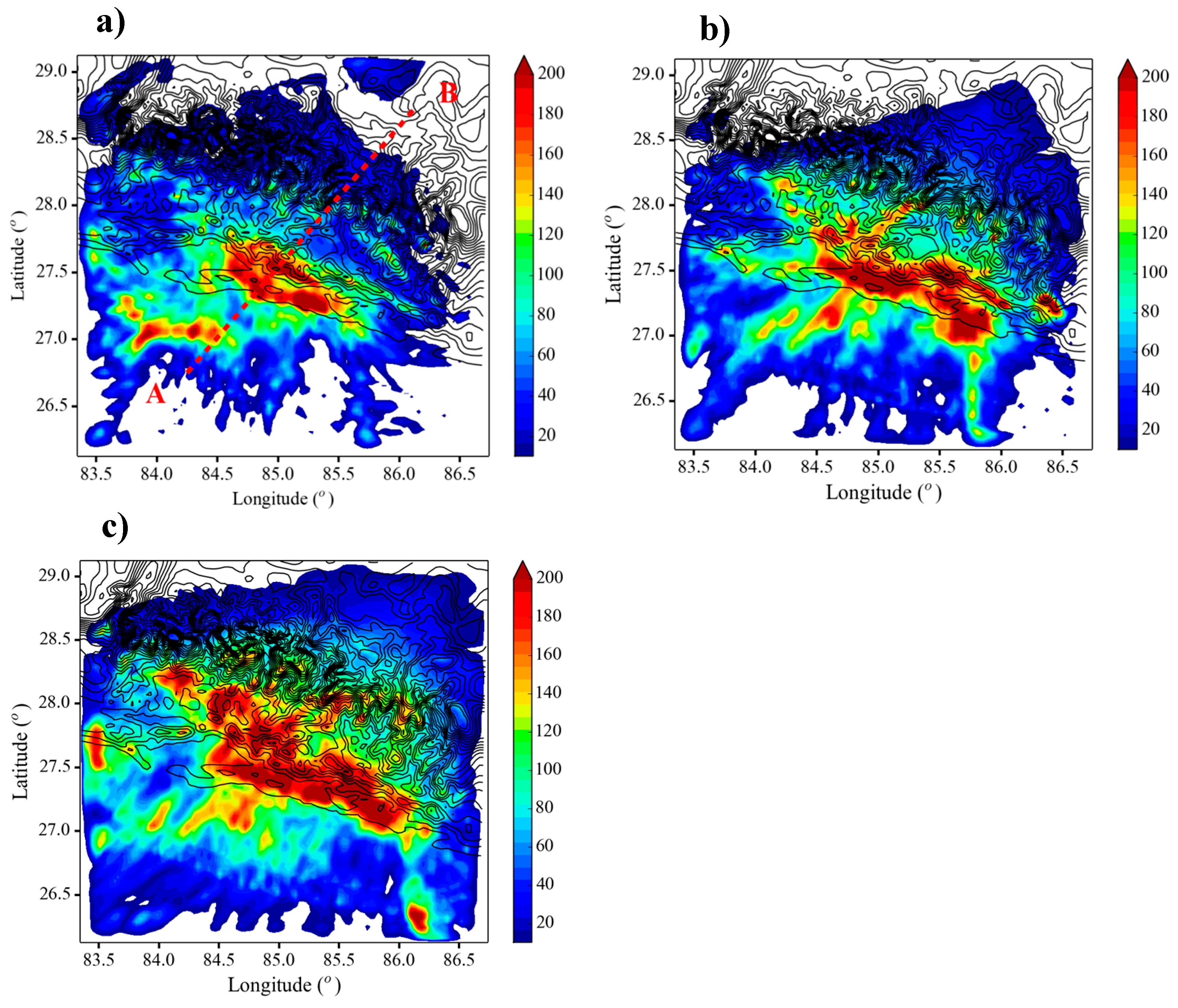
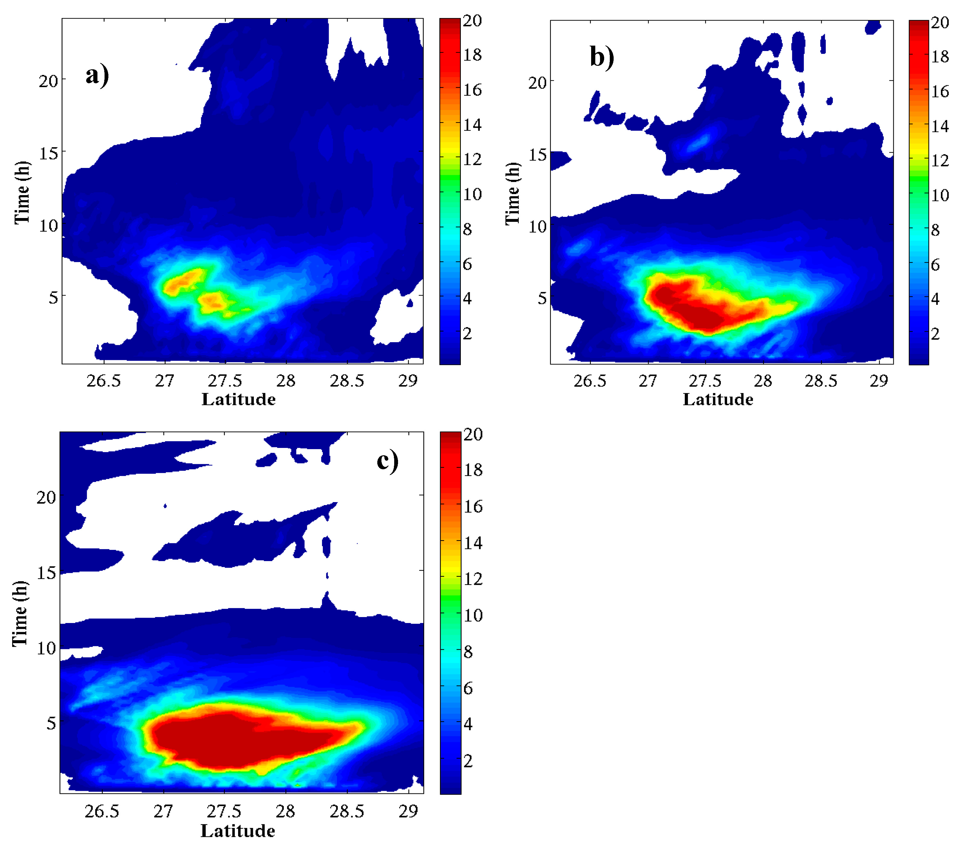
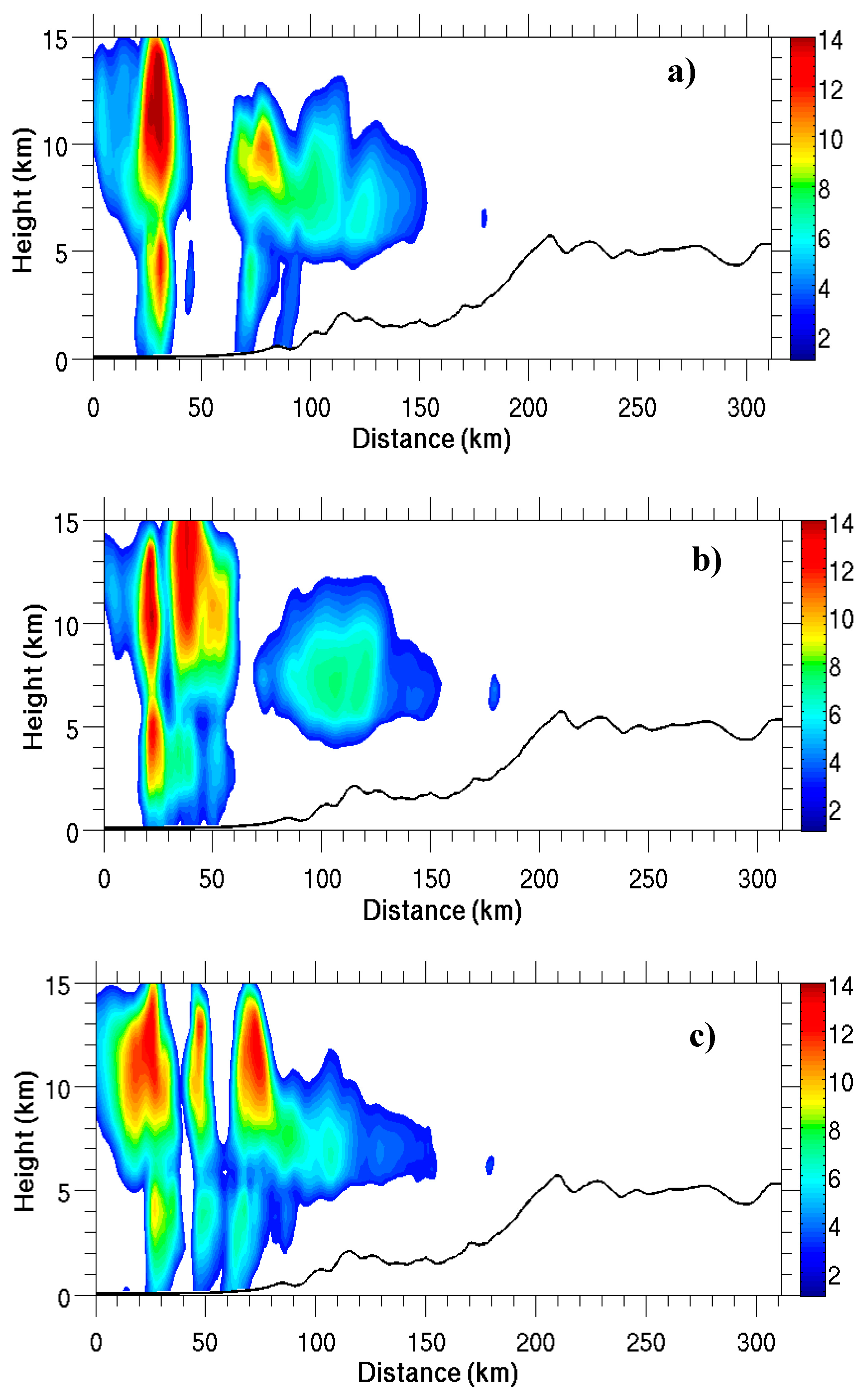
5.2. Distribution of Clouds and Rain

5.2.1. Case Study I

Hovmöller diagrams (Figure 4a–c) describe an evolution of hydrometeors over time along south—north direction of the domain. The spatial distribution of hydrometeors in the ‘low’, ‘medium’ and ‘high’ aerosol cases is not significantly different. In all cases, results show that a thick cloud band (~20 g kg−1) is developed across central Nepal (~27° N–~28° N) early in the simulation which gradually diminishes after ~8 h, however, thin clouds (<2 g kg−1) evolve almost everywhere from the beginning to the end of the simulations. In contrast, temperature perturbations show a significant impact on the distribution of clouds (Figure 4b–c). The thick band of cloud develops rapidly, spread out reaching almost to 29° N (South of the Tibetan Plateau), and sustains longer in the atmosphere. In contrast, the thin clouds do not survive until the end of simulations. In particular, this effect is prominent in the Tctrl + 10 run. A weak cloud band was observed in the Tctrl ± 0.5, Tctrl ± 2.5 and Tctrl ± 5 simulations.
Consistent with distribution of hydrometeors, the impact of aerosol perturbations on the distribution of rainfall is negligible and not statistically significant at the 95% confidence interval. In general, in all cases, a WNW–ESE oriented rainfall corridor was observed along the foothills of the Himalayas (Figure 5a). Results show that the foothills of the Himalayas (e.g., Siwalik Hills and Mahabharat Range; altitude 1500 m–4500 m) receive more rain than in the high Himalayas (altitude > 5000 m) and ‘Teari’ areas (southern low land, altitude < 200 m). Heavy rainfall is confined mostly across the windward side of two prominent peaks, Champadevi (85.25° E, 27.65° N; altitude: 2250 m) and Phulchowki (85.41° E, 27.57° N; altitude 2760 m), located SW–SE of the Kathmandu Valley.
Unlike aerosol, temperature perturbations show a significant impact on distribution of rainfall (Figure 5b,c) and statistically significant at the 95% confidence interval. An elongated rainfall corridor further encroaching northwest of the Himalayas was observed in the Tctrl + 5 and Tctrl + 10 simulations. A wider rainfall corridor covering a large geographical area in the central Nepal is developed, if temperature rises by 10 °C. The rain belt is relatively weak and not organized in the Tctrl ± 0.5, Tctrl ± 2.5 and Tctrl ± 5 runs.

5.2.2. Case Study II

The spatial distributions of hydrometeors are very similar in the ‘low’, ‘medium’ and ‘high’ aerosol cases (not shown). Consistent with case I, in all cases, a thick blanket of cloud is developed over central Nepal early in the simulations and disappears after ~8 h, however, thin clouds are found everywhere from the beginning to end of the simulations. Unlike aerosol, temperature perturbations show a considerable impact on the distribution of hydrometeors. The thick blanket of cloud develops rapidly, moves toward the high Himalayas and stays longer in the atmosphere with increase in temperature.
The impact of aerosol perturbations on the distribution of rainfall is not statistically significant at the 95% confidence interval. In all cases, consistent with case I, a WNW–ESE rainfall corridor was formed along the foothills of the Himalayas (not shown). The maximum amount of rainfall was observed across the Siwalik Hills and Mahabharat Range (altitude 1500 m–4500 m). In contrast, the impact of temperature perturbations on the distribution of rainfall is statistically significant at the 95% confidence interval. The rainfall corridor is further widened as temperature rises.

5.2.3. Case Study III

The distributions of hydrometeors are very similar between the ‘low’, ‘medium’ and ‘high’ aerosol cases (not shown). As this case is characterised by a low rainfall event the thick blanket of cloud, as observed in the previous cases, does not appear. Instead few patches of scattered clouds are observed from the beginning to the end of simulations.
Consistent with distribution of clouds, the impact of aerosol perturbations on the distribution of rainfall is minimal and not statistically significant at the 95% confidence interval. As this event is caused by a winter monsoon precipitation, which is influenced by extra-tropical cyclones, the high Himalayan region receives patches of light rains. The light rainfall area widens up and moves southward along the foothills of the Himalayas as the magnitude of the temperature perturbations increases. The impact of temperature perturbations on rainfall is statistically significant at the 95% confidence interval.

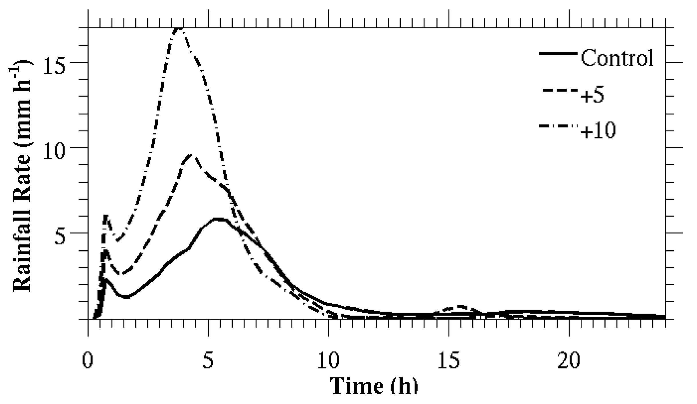
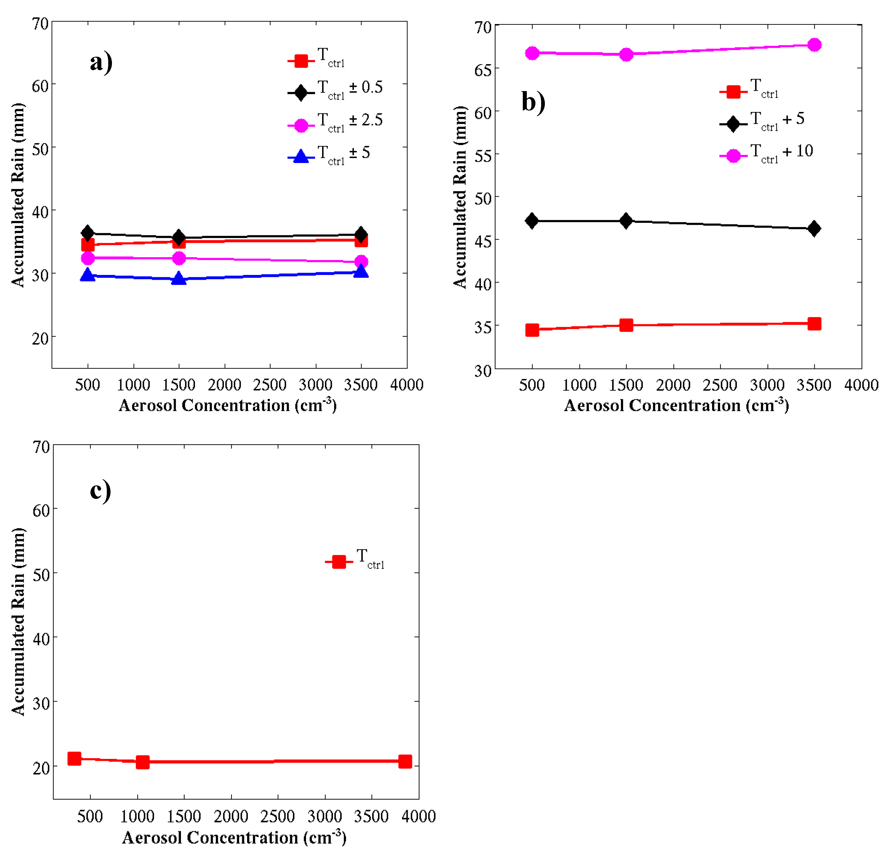
5.3. Precipitation Sensitivity to Aerosol and Temperature Perturbations

5.3.1. Case Study I

Figure 6a–c show the effects of aerosol and temperature perturbations on accumulated rainfall. The impact of aerosol perturbations was minimal ranging from −3% to +4%. The effect was non-linear and not statistically significant at the 95% confidence interval. However, temperature perturbations show greater impact on the rainfall (−5% to +93%), which was statistically significant at the 95% confidence interval. The decreased rainfall is attributed to the random perturbations of atmospheric temperature which randomly choose a grid box to add or subtract the perturbations on Tctrl. A summary of the accumulated rainfall from the sensitivity runs is presented in Table 3.
In the Tctrl runs, time series analysis show an early and rapid development of rain followed by an intense downpour that occurred for a short period of time (Figure 7), which is consistent with the evolution of clouds as shown in Hovmöller diagram (Figure 4). This feature of rainfall was also observed in Tctrl + 5 and Tctrl + 10 simulations, however, with more intense downpour. In contrast, although rainfall initiates at the same time, a more gradual evolution of rain was observed, consequently producing less intense and prolonged rainfall in the Tctrl ± 0.5, Tctrl ± 2.5 and Tctrl ± 5 simulations.
Figure 8a–c show a cross section of the total condensate (sum of cloud droplets, rain, cloud ice, snow and graupel) along the line AB in Figure 5a which was taken just before onset of rainfall for the ‘low’, ‘medium’ and ‘high’ aerosol perturbations. In the ‘low’ aerosol case a narrow condensate region, both horizontal and vertical distribution, with less hydrometeor content was observed. In contrast, in the ‘medium’ and ‘high’ aerosol cases, height of the condensate regions and its horizontal extents were significantly increased.

5.3.2. Case Study II

Consistent with the case I, the impact of aerosol perturbations on rainfall was not statistically significant at the 95% confidence interval and the effects were non-linear. In contrast, the effect of temperature perturbations, which was statistically significant at the 95% confidence interval, was estimated to range from −11% to +3%. Note that this effect is entirely due to the random perturbation of temperature profile, as the uniform perturbations cases are not simulated here. Consistent with distribution of clouds in the Hovmöller diagram, an early evolution of rain and its rapid growth was observed in the time series analysis of rainfall, which subsequently generates high intensity rainfall over a short period of time. The maximum rainfall occurred ~5 h of simulation in the Tctrl run, which gradually shifted farther in the Tctrl ± 0.5, Tctrl ± 2.5 and Tctrl ± 5 simulations. Analysis of individual cloud regions show that the cloud could extend up to 18 km from the ground level, where freezing level generally exist around 5 km, indicates a dominance of cold phase hydrometeors.

5.3.3. Case Study III

Amount of rainfall are very similar in the all aerosol perturbation scenarios. Hence, the impact of aerosol perturbations on rainfall is not statistically significant at the 95% confidence interval. Note that this event is characterised by a low intensity rain during a winter season as explained above. However, a strong sensitivity of rainfall to the temperature perturbations (−1% to +22%) was observed. Consistent with distribution of clouds in the Hovmöller diagram, time series analysis of rainfall shows that onset timing is very similar in all the simulations. However, gradual evolution of the rain, as compared to Tctrl, was observed in the perturbed simulations. Shape, size and spatial distribution of the total condensate are very similar in the ‘low’, ‘medium’, and ‘high’ aerosol cases, which were mostly dominated by ice phase hydrometeors.

6. Discussion and Conclusions

In this study we use a high resolution (3 km × 3 km) Weather Research and Forecasting (WRF) model to simulate the effects of aerosol and temperature perturbations on the distribution of clouds and precipitation over the Himalayas. Rainfall sensitivity was analyzed for three different case studies, accompanied with varying rainfall intensity and different season of a year, in order to draw more robust conclusions. We compare the simulated results from control runs to experimental runs which were created perturbing atmospheric temperature profiles using both (i) uniform; and (ii) random perturbations, for three different ‘low’, ‘medium’ and ‘high’ aerosol perturbation scenarios.
The cloud droplets number concentrations are positively correlated to aerosol number concentrations, as expected. However, as explained above the effects of aerosol perturbations are non-linear. This non-linear effect of aerosol was also observed in the convective clouds over India [48] attributed to increased droplets concentration, due to higher CCN concentration, which compete for available water vapour, in turn, reduce supersaturation [39]. Ice crystal number concentration is not significantly affected by the aerosol perturbations. The poor sensitivity of the ice concentration is attributed to the oversimplified parameterizations scheme of ice nucleation processes, where chemical properties of aerosol particles that play a critical role to determine particle’s ice nucleation behaviour [49,50] are not considered. Although the droplet size is decreased with increasing aerosol number concentration, the size of the cloud ice is generally increased, which may be associated with the ‘glaciation’ indirect effect. In this mechanism ice particles grow at the expense of cloud droplets due to its lower saturation vapour pressure [20,51]. However, this feature is less robust as it is not supported by all scenarios.
Our results show that the amount of rainfall is not overly sensitive to aerosol perturbations (−3% to +4%) and not statistically significant at the 95% confidence interval. Consistent with droplets concentration the effect of aerosol on rainfall is non-linear, the similar effect was also observed in the deep tropical convection [47]. The insensitivity of rainfall to aerosol perturbations over the Himalayas can be explained in two ways. Firstly, ice phase is the dominant precipitation formation processes over the mountainous region [52], this mechanism was also observed in our simulations as the ratio of liquid water content (LWC) to ice water content (IWC) ranges from 0.5 to 0.9. However, the ice phase processes are not sensitive to the aerosol perturbations as explained above that have a strong influence on the sensitivity to rainfall. The same effect was also observed in Alps and Rocky Mountains [50]. Secondly, the ice phase clouds could compensate the suppressed warm rain via melting of ice hydrometeors [28].
Spatial distributions of rainfall show that the foothills of the Himalayas (e.g., Siwalik Hills and Mahabharat Range; altitude 1500 m–4500 m) receive more rain as compared to the high Himalayas (altitude > 5000 m) and ‘Teari’ region (southern low land, altitude < 200 m). This feature is consistent with all the aerosol perturbation scenarios. A WNW—ESE oriented rainfall corridor is observed along the foothills of the Himalayas, confining heavy rainfall mostly across the windward side of two prominent peaks (i.e., Champadevi and Phulchowki; altitude 2500–2700 m) located SW—SE of the Kathmandu Valley. These are well understood properties of orographic rain attributed to the complex mountainous terrain [53] where warm and moist air is forced up to high elevation resulting in cooling and condensation/precipitation along the windward slope of the topographic barrier and subsidence in the leeward side evaporates the clouds.
Intense rainfall over the foothills of the Himalayas is observed in a warming climate which sustained for a very short period of time. The magnitudes of such effects are more pronounced with rising temperatures, for example, +31% to +93% more rain will be produced if the temperature is increased by 5 °C to 10 °C. The increased rainfall amount is associated with increase in atmospheric moisture due to increased temperature, the Clausius–Clapeyron effect, which suggests that at constant relative humidity moisture content increases by ~6%/K near surface and ~12%/K in the upper troposphere [13]. Thus, it is likely that the Indian monsoon precipitation will intensify as the climate warms which is also suggested by Turner and Annamalai [2].
Analysis of total condensate (i.e., sum of cloud droplets, rain, cloud ice, snow and graupel) shows that aerosol perturbations are likely to modify shape, size and spatial distribution of hydrometeors and their precipitation production at individual cloud region. However, in some cases, presented in this study, low intensity rainfall during winter season is not affected at all by the aerosol perturbations. This could be attributed to a weak response of ice phase processes to the aerosol perturbations. So the resulting effects of aerosols on cloud processing, spatial distribution and precipitation onset can be highly non-linear and case dependent.

Author Contributions

P.J.C. and M.W.G. designed the experiment and reviewed the manuscript. R.K.S. performed the experiment, analyzed the data, created the figures and wrote the paper. All authors have read and agreed to the published version of the manuscript.

Acknowledgments

This project was carried out under the funding of Sustainable Consumption Institute (SCI), University of Manchester. The authors would like to thank SCI for PhD funding.

Conflicts of Interest

The authors declare no conflict of interest.

References

  1. Mooley, D.A.; Parthasarathy, B. Fluctuations in All-India summer monsoon rainfall during 1871–1978. Clim. Chang. 1984, 6, 287–301. [Google Scholar] [CrossRef]
  2. Turner, A.G.; Annamalai, H. Climate change and the South Asian summer monsoon. Nat. Clim. Chang. 2012, 2, 587–595. [Google Scholar] [CrossRef]
  3. Duncan, J.M.A.; Biggs, E.M.; Dash, J.; Atkinson, P.M. Spatio-temporal trends in precipitation and their implication for water resources management in climate-sensitive Nepal. Appl. Geogr. 2013, 43, 138–146. [Google Scholar] [CrossRef]
  4. Webster, P.J.; Magana, V.O.; Palmer, T.N.; Shukla, J.; Tomas, R.A.; Yanai, M.U.; Yasunari, T. Monsoons: Processes, predictability, and the prospects for prediction. J. Geophys. Res. 1998, 103, 14451–14510. [Google Scholar] [CrossRef]
  5. Li, J.; Wang, B.; Yang, Y.-M. Retrospective seasonal prediction of summer monsoon rainfall over West Central and Peninsular India in the past 142 years. Clim Dyn. 2016, 48, 2581–2596. [Google Scholar] [CrossRef]
  6. Kumar, K.K.; Kumar, K.R.; Ashrit, R.G.; Deshpande, N.R.; Hansen, J.W. Climate Impacts on Indian agriculture. Int. J. Climatol. 2004, 24, 1375–1393. [Google Scholar] [CrossRef]
  7. Reuter, M.; Kern, A.K.; Harzhauser, M.; Kroh, A.; Piller, W.E. Global warming and South Indian monsoon rainfall - lessons from the Mid-Miocene. Gondwana Res. 2013, 23, 1172–1177. [Google Scholar] [CrossRef]
  8. Das, L.; Meher, J.K.; Dutta, M. Construction of rainfall change scenarios over teh Chilka Lagoon in India. Atmos. Res. 2016, 182, 36–45. [Google Scholar] [CrossRef]
  9. IPCC. Climate Change 2014: Synthesis Report. Contribution of Working Groups I, II and III to the Fifth Assessment Report of the Intergovernmental Panel on Climate Change; IPCC: Geneva, Switzerland, 2014; 151p. [Google Scholar]
  10. Liu, X.; Chen, B. Climatic warming in the Tibetan Plateau during recent decades. Int. J. Climatol. 2000, 20, 1729–1742. [Google Scholar] [CrossRef]
  11. Shrestha, A.B.; Wake, C.P.; Mayewski, P.A.; Dibb, J.E. Maximum Temperature Trends in the Himalaya and Its Vicinity: An Analysis Based on Temperature Records from Nepal for the Period 1971–94. J. Clim. 1999, 12, 2775–2786. [Google Scholar] [CrossRef]
  12. Ghatak, D.; Sinsky, E.; Miller, J. Role of snow-albedo feedback in higher elevation warming over the Himalayas, Tibetan Plateau and Central Asia. Environ. Res. Lett. 2014, 9, 114008. [Google Scholar] [CrossRef]
  13. Soden, B.J.; Jackson, D.L.; Ramaswamy, V.; Schwarzkopf, M.D.; Huang, X. The Radiative Signature of Upper Tropospheric Moistening. Science 2005, 310, 841–844. [Google Scholar] [CrossRef] [PubMed]
  14. Gautam, R.; Hsu, N.C.; Lau, K.-M.; Kafatos, M. Aerosol and rainfall variability over the Indian monsoon region: Distributions, trends and coupling. Ann. Geophys. 2009, 27, 3691–3703. [Google Scholar] [CrossRef]
  15. Wang, C.; Kim, D.; Ekman, A.M.L.; Barth, M.C.; Rasch, P.J. Impact of anthropogenic aerosols on Indian summer monsoon. Geophys. Res. Lett. 2009, 36, L21704. [Google Scholar] [CrossRef]
  16. Twomey, S. The influence of pollution on the shortwave albedo of clouds. J. Atmos. Sci. 1977, 34, 1149–1152. [Google Scholar] [CrossRef]
  17. Albrecht, B.A. Aerosols, Cloud Microphysics, and Fractional Cloudiness. Science 1989, 245, 1227–1230. [Google Scholar] [CrossRef]
  18. Demott, P.J.; Chen, Y.; Kreidenweis, S.M.; Rogers, D.C.; Sherman, D.E. Ice formation by black carbon particles. Geophys. Res. Lett. 1999, 26, 2429–2432. [Google Scholar] [CrossRef]
  19. DeMott, P.J.; Prenni, A.J.; Liu, X.; Kreidenweis, S.M.; Petters, M.D.; Twohy, C.H.; Richardson, M.S.; Eidhammer, T.; Rogers, D.C. Predicting global atmospheric ice nuclei distributions and their impacts on climate. Proc. Natl. Acad. Sci. USA 2010, 107, 11217–11222. [Google Scholar] [CrossRef]
  20. Lohmann, U.; Feichter, J. Global indirect aerosol effects: A review. Atmos. Chem. Phys. 2005, 5, 715–737. [Google Scholar] [CrossRef]
  21. Wang, B. The Asian Monsoon; Praxis Publishing Ltd.: Chichester, UK, 2006. [Google Scholar]
  22. Houze, R.A.; Wilton, D.C.; Smull, B.F. Monsoon convection in the Himalayan region as seen by the TRMM Precipitation Radar. Q. J. R. Meteorol. Soc. 2007, 133, 1389–1411. [Google Scholar] [CrossRef]
  23. Shrestha, P.; Barros, A.P.; Khlystov, A. Chemical composition and aerosol size distribution of the middle mountain range in the Nepal Himalayas during the 2009 pre-monsoon season. Atmos. Chem. Phys. 2010, 10, 11605–11621. [Google Scholar] [CrossRef]
  24. Lynn, B.; Khain, A.; Rosenfeld, D.; Woodely, W.L. Effect of aerosols on precipitation from orographic clouds. J. Geophys. Res. 2007, 112, D10225. [Google Scholar] [CrossRef]
  25. Jirak, I.L.; Cotton, W.R. Effects of air pollution on precipitation along the front range of the Rocky Mountains. J. Appl. Meteorol. Climatol. 2006, 45, 236–245. [Google Scholar] [CrossRef]
  26. Muhlbauer, A.; Lohmann, U. Sensitivity Studies of the Role of Aerosols in Warm-Phase Orographic Precipitation in Different Dynamical Flow Regimes. J. Atmos. Sci. 2008, 65, 2522–2541. [Google Scholar] [CrossRef]
  27. Collins, M.R.; Knutti, J.A.; Dufresne, J.-L.; Fichefet, T.; Friedlingstein, P.; Gao, X.; Gutowski, W.J.; Johns, T.; Krinner, G.; Shongwe, M.; et al. Long-term Climate Change: Projections, Commitments and Irreversibility. In Climate Change 2013: The Physical Science Basis. Contribution of Working Group I to the Fifth Assessment Report of the Intergovernmental Panel on Climate Change; Cambridge University Press: Cambridge, UK; New York, NY, USA, 2013. [Google Scholar]
  28. Lee, S.-S.; Feingold, G. Precipitating cloud-system response to aerosol perturbations. Geophys. Res. Lett. 2010, 37, L23806. [Google Scholar] [CrossRef]
  29. Klemp, J.B.; Dudhia, J.; Hassiotis, A. An Upper Gravity Wave Absorbing Layer for NWP Applications. Mon. Weather Rev. 2008, 136, 3987–4004. [Google Scholar] [CrossRef]
  30. Skamarock, W.C.; Klemp, J.B.; Dudhia, J.; Grill, D.O.; Barker, D.M.; Duda, M.G.; Huang, X.Y.; Wang, W.; Powers, J.G. A Description of the Advanced Research WRF Version 3; Technical Report; National Center for Atmospheric Research: Boulder, CO, USA, 2008; 113p. [Google Scholar]
  31. Shrestha, R.K.; Connolly, P.J.; Gallagher, M.W. Sensitivity of WRF cloud microphysics to simulations of a convective storm over the Nepal Himalayas. Open Atmos. Sci. J. 2016, submitted. [CrossRef]
  32. Jimenez, P.A.; Gonzalez-Rouco, J.F.; Gracia-Bustamante, E.; Navarro, J.; Nontavez, J.P.; De Arellano, J.V.G.; Dudhia, J.; Muñoz-Roldan, A. SurfaceWind Regionalization over Complex Terrain: Evaluation and Analysis of a High-Resolution WRF Simulation. J. Appl. Meteorol. Clim. 2010, 49, 268–287. [Google Scholar] [CrossRef]
  33. Ikeda, K.; Rasmussen, R.; Liu, C.; Gochis, D.; Yates, D.; Chen, F.; Tewari, M.; Barlage, M.; Dudhia, J.; Miller, K.; et al. Simulation of seasonal snowfall over Colorado. Atmos. Res. 2010, 97, 462–477. [Google Scholar] [CrossRef]
  34. Rasmussen, R.; Liu, C.; Ikeda, K.; Gochis, D.; Yates, D.; Chen, F.; Tewari, M.; Barlage, M.; Dudhia, J.; Yu, W.; et al. High-resolution coupled climate runoff simulations of seasonal snowfall over Colorado: A process study of current and warmer climate. J. Clim. 2011, 24, 3015–3048. [Google Scholar] [CrossRef]
  35. Liu, C.; Ikeda, K.; Rasmussen, R.; Barlage, M.; Newman, A.J.; Prein, A.F.; Chen, F.; Chen, L.; Clark, M.; Dai, A.; et al. Continental-scale convection-permitting modeling of the current and future climate of North America. Clim. Dyn. 2016, 49, 71–95. [Google Scholar] [CrossRef]
  36. Maussion, F.; Scherer, D.; Finkelnburg, R.; Richters, J.; Yang, W.; Yao, T. WRF simulation of a precipitation event over the Tibetan Plateau, China—And assessment using remote sensing and ground observations. Hydrol. Earth Syst. Sci. Dissuss. 2010, 7, 3551–3589. [Google Scholar] [CrossRef]
  37. Morrison, H.; Curry, J.A.; Khvorostyanov, V.I. A New Double-Moment Microphysics Parameterization for Application in Cloud and ClimateModels. Part I: Description. J. Atmos. Sci. 2005, 62, 1665–1676. [Google Scholar] [CrossRef]
  38. Morrison, H.; Thompson, G.; Tatarskii, V. Impact of Cloud Microphysics on the Development of Trailing Stratiform Precipitation in a Simulated Squall Line: Comparison of One- and Two-Moment Schemes. Mon. Weather Rev. 2009, 137, 991–1007. [Google Scholar] [CrossRef]
  39. Twomey, S. The nuclei of natural cloud formation part II: The supersaturation in natural clouds and the variation of cloud droplet concentration. Geofisica Pura Appl. 1959, 43, 243–249. [Google Scholar] [CrossRef]
  40. Rogers, R.R.; Yau, M.K. A short Course in Cloud Physics, 3rd ed.; Pergamon Press: Oxford, UK; New York, NY, USA, 1989. [Google Scholar]
  41. Khairoutdinov, M.; Kogan, Y. A new Cloud Physics Parameterization in a Large-Eddy Simulation Model of Marine Stratocumulus. Mon. Weather Rev. 2000, 128, 229–243. [Google Scholar] [CrossRef]
  42. Rasmussen, R.M.; Geresdi, I.; Thompson, G.; Manning, K.; Karplus, E. The Role of Radiative Cooling of Clouds Droplets, Cloud Condensation Nuclei, and Ice Initiation. J. Atmos. Sci. 2002, 59, 837–860. [Google Scholar] [CrossRef]
  43. Hallett, J.; Mossop, S.C. Production of secondary ice particles during the riming process. Nature 1974, 249, 26–28. [Google Scholar] [CrossRef]
  44. Dudhia, J. Numerical study of convection observed during the winter monsoon experiment using a mesoscale two-dimensional model. J. Atmos. Sci. 1989, 46, 3077–3107. [Google Scholar] [CrossRef]
  45. Mlawer, E.J.; Taubman, S.J.; Brown, P.D.; Iacono, M.J.; Clough, S.A. Radiative transfer for inhomogeneous atmosphere: RRTM, a validated correlated-k model for the longwave. J. Geophys. Res. 1997, 102, 16663–16682. [Google Scholar] [CrossRef]
  46. Hong, S.Y.; Noh, Y.; Dudhia, J. A new vertical diffusion package with an explicit treatment of entrainment processes. Mon. Weather Rev. 2006, 143, 2318–2341. [Google Scholar] [CrossRef]
  47. Connolly, P.J.; Vaughan, G.; May, P.T.; Chemel, C.; Allen, G.; Choularton, T.W.; Gallagher, M.W.; Bower, K.N.; Crosier, J.; Dearden, C. Can aerosol influence deep tropical convection? Aerosol indirect effects in the Hector island thunderstorm. Q. J. R. Meteorol. Soc. 2013, 139, 2190–2208. [Google Scholar] [CrossRef]
  48. Konwar, M.; Maheskumar, R.S.; Kulkarni, J.R.; Freud, E.; Goswami, B.N.; Rosenfeld, D. Aerosol control on depth of warm rain in convective clouds. J. Geophys. Res. 2012, 117, D13204. [Google Scholar] [CrossRef]
  49. Pruppacher, H.R.; Klett, J.D. Microphysics of Clouds and Precipitation; Atmospheric and Oceanographic Sciences Library, Kluwer Academic Publishers: Dordrecht, The Netherlands, 1997. [Google Scholar]
  50. Muhlbauer, A.; Hashino, T.; Xue, L.; Teller, A.; Lohmann, U.; Rasmussen, R.M.; Geresdi, I.; Pan, Z. Intercomparison of aerosol-cloud-precipitation interaction in stratiform orographic mixed-phase clouds. Atmos. Chem. Phys. 2010, 10, 8173–8196. [Google Scholar] [CrossRef]
  51. Connolly, P.J.; Choularton, T.W.; Gallagher, W.W.; Bower, K.N.; Flynn, M.J.; Whiteway, J.A. Cloud-resolving simulations of intense tropical Hector thunderstorms:Implications for aerosol cloud interactions. Q. J. R. Meteorol. Soc. 2006, 132, 3079–3106. [Google Scholar] [CrossRef]
  52. Chen, J.-P.; Lamb, D. Simulation of cloud microphysical and chemical processes using a multicomponent framework. Part II: Microphysical evolution of a wintertime orographic cloud. J. Atmos. Sci. 1999, 56, 2293–2312. [Google Scholar] [CrossRef]
  53. Barros, A.P.; Lettenmaier, D.P. Dynamic Modeling of Orographically Induced Precipitation. Rev. Geophys. 1994, 32, 265–284. [Google Scholar] [CrossRef]
Figure 1. Domains used for WRF simulation with horizontal grid resolution 27 km (domain 1), 9 km (domain 2) and 3 km (domain 3) centered over central Nepal (26.34° N, 83.12° E) and the model is set to 40 vertical levels. Elevation contours are plotted at intervals of 500 m between 1500 and 8000 m altitudes.
Proceedings 01 00144 g001
Figure 2. Correlation between cloud droplet number concentration (CDNC) and aerosol concentrations simulated for (a) random temperature perturbations; (b) uniform temperature perturbations; and (c) prognostic CCN scenarios; (d) Correlation between ice number concentration and aerosol concentration simulated for uniform temperature perturbations.
Proceedings 01 00144 g002
Figure 3. Correlation between domain and time averaged updraft speed (Wa) and CDNC in the uniform temperature perturbation along the north–south transect of the domain. Average CDNC is calculated for positive mean vertical velocity (Wa > 0) in the corresponding grid box of the model. L, M and H in the legend stands for the ‘low’, ‘medium’, and ‘high’ aerosol cases, respectively.
Proceedings 01 00144 g003
Figure 4. Hovmöller diagrams for total condensate (g kg1) simulated for the ‘low’ aerosol concentration (a) Tctrl; (b) Tctrl + 5 °C; and (c) Tctrl + 10 °C. As explained in the text, this diagram is very similar for the ‘medium’ and ‘high’ aerosol concentrations.
Proceedings 01 00144 g004
Figure 5. Spatial distribution of rainfall simulated for the ‘low’ aerosol concentration (a) Tctrl; (b) Tctrl + 5 °C; and (c) Tctrl + 10 °C. As explained in the text, this diagram is very similar for the ‘medium’ and ‘high’ aerosol concentrations. Elevation contours are plotted at intervals of 300 m between 300 and 6000 m altitudes.
Proceedings 01 00144 g005
Figure 6. Sensitivity of accumulated rain to aerosol and temperature perturbations (a) random temperature perturbation; (b) uniform temperature perturbation; and (c) prognostic CCN scenarios.
Proceedings 01 00144 g006
Figure 7. Time series analysis of accumulated rainfall, which is averaged over the domain simulated for the ‘low’ aerosol concentration. As explained in the text, this diagram is very similar for the ‘medium’ and ‘high’ aerosol concentrations.
Proceedings 01 00144 g007
Figure 8. Distribution of total condensate (g kg−1) along line AB in the Figure 5a for (a) ‘low’; (b) ‘medium’; and (c) ‘high’ aerosol concentration simulated for the Tctrl simulation. These cross-sections were taken at 4:45 GMT (10:30 am local time), just before onset of the rainfall.
Proceedings 01 00144 g008
Table 1. Inter-comparison of domain and time averaged cloud droplet effective radius (μm). Dashes indicate no simulations were performed for the case.
SimulationCase-ICase-IICase-III
LowMediumHighLowMediumHighLowMediumHigh
Control (Tctrl)14.8514.8014.7714.8414.8214.7815.2115.2115.21
Uniform temperature perturbation
Tctrl + 514.9514.9114.90------
Tctrl + 1014.9314.8914.86------
Random temperature perturbation
Tctrl ± 0.514.8414.8114.7614.8514.8214.7915.2115.2115.21
Tctrl ± 2.514.8514.8214.7814.8514.8214.8015.2115.2115.21
Tctrl ± 514.8114.7514.7214.8214.7814.7715.2115.2115.21
Prognostic CCN14.5814.6414.58------
Table 2. Same as Table 1 but for the ice effective radius (μm).
SimulationCase-ICase-IICase-III
LowMediumHighLowMediumHighLowMediumHigh
Control (Tctrl)38.4538.6638.7431.2031.1431.2626.4326.4326.44
Uniform temperature perturbation
Tctrl + 535.4835.6035.26------
Tctrl + 1037.1237.3636.89------
Random temperature perturbation
Tctrl ± 0.538.9738.8938.8331.5131.4531.3426.4426.4426.44
Tctrl ± 2.539.0039.1639.1631.8231.8131.7726.5426.5426.54
Tctrl ± 539.0539.1939.2632.5632.5032.4526.5726.5726.58
Prognostic CCN29.8729.3629.22------
Table 3. Inter-comparison of accumulated rainfall (mm). Dashes indicate no simulations were performed for the case.
SimulationCase-ICase-IICase-III
LowMediumHighLowMediumHighLowMediumHigh
Control (Tctrl)34.535.035.251.851.050.90.30.30.3
Uniform temperature perturbation
Tctrl + 547.147.146.2------
Tctrl + 1066.766.667.7------
Random temperature perturbation
Tctrl ± 0.536.335.636.153.152.152.30.30.30.3
Tctrl ± 2.532.432.431.847.948.148.00.30.30.3
Tctrl ± 529.629.030.246.045.945.40.40.40.4
Prognostic CCN21.120.620.7------
Publisher’s Note: MDPI stays neutral with regard to jurisdictional claims in published maps and institutional affiliations.

