Article

Estimation Method of Leaf Nitrogen Content of Dominant Plants in Inner Mongolia Grassland Based on Machine Learning

1
The College of Resources and Environmental Engineering, Inner Mongolia University of Technology, Hohhot 010051, China
2
The College of Ecology and Environment, Inner Mongolia University, Hohhot 010021, China
*
Authors to whom correspondence should be addressed.
Nitrogen 2025, 6(3), 70; https://doi.org/10.3390/nitrogen6030070
Submission received: 18 July 2025 / Revised: 15 August 2025 / Accepted: 18 August 2025 / Published: 19 August 2025

Abstract

Accurate nitrogen (N) content estimation in grassland vegetation is essential for ecosystem health and optimizing pasture quality, as N supports plant photosynthesis and water uptake. Traditional lab methods are slow and unsuitable for large-scale monitoring, while remote sensing models often face accuracy challenges due to hyperspectral data complexity. This study improves N content estimation in the typical steppe of Inner Mongolia by integrating hyperspectral remote sensing with advanced machine learning. Hyperspectral reflectance from Leymus chinensis and Cleistogenes squarrosa was measured using an ASD FieldSpec-4 spectrometer, and leaf N content was measured with an elemental analyzer. To address high-dimensional data, four spectral transformations—band combination, first-order derivative transformation (FDT), continuous wavelet transformation (CWT), and continuum removal transformation (CRT)—were applied, with Least Absolute Shrinkage and Selection Operator (LASSO) used for feature selection. Four machine learning models—Extreme Gradient Boosting (XGBoost), Support Vector Machine (SVM), Artificial Neural Network (ANN), and K-Nearest Neighbors (KNN)—were evaluated via five-fold cross-validation. Wavelet transformation provided the most informative parameters. The SVM model achieved the highest accuracy for L. chinensis (R2 = 0.92), and the ANN model performed best for C. squarrosa (R2 = 0.72). This study demonstrates that integrating wavelet transform with machine learning offers a reliable, scalable approach for grassland N monitoring and management.

1. Introduction

Grasslands play a vital role in terrestrial ecosystems and represent the most extensively distributed form of land cover [1,2,3]. Globally, natural grasslands account for 41.7% of the total land area. These grassland resources fulfill numerous significant ecological functions, including sand stabilization, water retention, biodiversity preservation, climate moderation, carbon sequestration, and serving as carbon sinks. Moreover, they provide a crucial ecological and material foundation for environmental protection and the support of biological life [4]. A strong correlation exists between the nitrogen content in vegetation and the net primary productivity of plants; a gradual decline in nitrogen content can impede plant photosynthesis, which is essential for growth and reproduction [5,6]. Therefore, a precise and comprehensive assessment of nitrogen levels in grassland vegetation is crucial for refining fertilizer use, enhancing pasture productivity, reducing ecological risks, and fostering the long-term sustainability of both grassland ecosystems and livestock production [7,8].
With the rise of hyperspectral remote sensing technology, due to its high spectral resolution and ability to provide abundant spectral information of ground objects, it has become a crucial tool for current vegetation nitrogen content inversion. Therefore, many scholars have investigated the spectral transformation and extraction of spectral features. Gao et al. [9] created a multivariate model aimed at estimating nitrogen levels in alpine grassland pasture ecosystems throughout the growing season. The optimal combination of 38 spectral variables, which effectively represents the dynamic fluctuations in pasture nitrogen, was identified using the random forest (RF) algorithm. Poonsak et al. [10] converted the initial spectral reflectance into first-order derivative spectra (FDS) and absorption characteristics to minimize spectral noise, utilizing these as input variables. Subsequently, they developed stepped multiple linear regression (SMLR) and support vector regression (SVR) models for the calibration and validation of the canopy nitrogen concentration (CNC) estimation model. The findings indicated that the estimation model based on the radial basis function (RBF) kernel using nonlinear SVR exhibited a significantly higher correlation coefficient with CNC compared to the SMLR model. Guo et al. [11] investigated various types of winter wheat as subjects for their research. They employed the continuum removal (CR) technique to enhance the N-absorption characteristic band and examined its relationship with leaf N accumulation, subsequently comparing the predictive accuracy of three nonlinear modeling approaches. The findings revealed that the CR method improved the correlation between the N-absorption characteristic band and leaf N accumulation, while also increasing the precision of estimating leaf N accumulation. Yu et al. [12] investigated the correlation between rice nitrogen levels and variations in spectral reflectance, developing a model based on hyperspectral reflectance differences to estimate rice nitrogen content. They performed a multiscale decomposition of hyperspectral data using discrete wavelet analysis, extracting essential wavelet coefficients through the continuous projection algorithm, which were subsequently employed as input parameters in their modeling process. The results demonstrated that the model created by the genetic algorithm–extreme learning machine (GA-ELM), which integrated the discrete wavelet multiscale decomposition, achieved the highest accuracy, explaining 68% of the variance in rice nitrogen content.
However, current research still faces many challenges. Hyperspectral data exhibit a substantial volume and high band dimension, with the potential for invalid, redundant, and overlapping spectral information. These factors contribute to the instability of the full-band inversion model and pose challenges in enhancing its accuracy. Moreover, the characteristics of different plant species vary. The existing research lacks in-depth exploration of spectral information, and the models’ accuracy is low, hindering their widespread application in accurately estimating nitrogen content in various grassland vegetation.
To address these challenges, this study develops and evaluates advanced methods for estimating leaf nitrogen content (LNC) in the typical steppe of Inner Mongolia, focusing on Leymus chinensis and Cleistogenes squarrosa. Hyperspectral reflectance data were collected from 200 leaf samples per species using a portable ASD FieldSpec-4 spectrometer (350–2500 nm), with nitrogen content measured via an elemental analyzer. Four dimensionality reduction methods—band combination, first-order derivative transformation (FDT), continuous wavelet transformation (CWT), and continuum removal transformation (CRT)—were applied to preprocess the data. Variable selection was performed using the Least Absolute Shrinkage and Selection Operator (LASSO) to identify the most informative spectral features. Four machine learning models—Extreme Gradient Boosting (XGBoost), Support Vector Machine (SVM), Artificial Neural Network (ANN), and K-Nearest Neighbors (KNN)—were developed and evaluated using five-fold cross-validation.
The method proposed in this study suggests that integrating wavelet transformation and machine learning techniques has the potential to enhance the accuracy of hyperspectral-based nitrogen content estimation for specific grassland species. This research aims to provide a comprehensive framework for hyperspectral-based nitrogen content estimation, customized for specific grassland species and environmental conditions. The findings are expected to offer valuable insights into improving grassland management and fertilization practices, thereby supporting sustainable development in arid and semi-arid regions.

2. Materials and Methods

2.1. Overview of the Study Area and Experimental Design

This study was conducted in August 2022 at the Grassland Ecology Research Base of Inner Mongolia University, located in Xilinhot, Inner Mongolia Autonomous Region, China (N 44°12.621′, E 116°15.446′). Situated in the Xilin Gol League, this site is a representative example of the typical steppe ecosystem in China’s temperate zone, characterized by its semi-arid climate and diverse grassland vegetation. The region experiences a temperate semi-arid continental climate with hot, rainy summers and cold, dry winters. The annual average temperature is 3.5 °C, with a frost-free period of 90–150 days. Annual precipitation averages 270 mm, with 87.3% occurring from May to September, coinciding with the peak growing season. The terrain features low hills and inter-hill flats. The soil is a chestnut according to the Chinese classification, or Haplic Calcisols according to the World Reference Base for Soil Resources (WRB) classification [13]. The vegetation is dominated by Chinese leymus as the constructive species, alongside Spreading Cleistogenes and Krylov’s Feather Grass as dominant species [14].
The sampling area covered approximately 1400 m2 and is divided into 40 plots measuring 5 m × 5 m. Two mowing treatments (mowing stubble left at 6 cm mowing with stubble left at 6 cm, CK control) and four fertilization treatments (N0P0 control, N1P0 with 100 kg ha−1 of N, N0P1 with 30 kg ha−1 of P, N1P1 with 100 kg ha−1 of N, and N1P1 with 30 kg ha−1 of P) were set up. Urea and calcium superphosphate served as sources of nitrogen and phosphorus fertilizers, and they were all applied at the same time as a basal fertilizer without any further applications. The experiment included 8 distinct treatments, with each treatment represented by 5 replicate blocks, leading to a total of 40 treatment plots. Figure 1 illustrates the study area and plot layout, providing a visual representation of the experimental design.

2.2. Data Observation

The experiment was conducted in August 2022, and two sets of samples were collected from each plot, each containing five plants of L. chinensis and three clumps of C. squarrosa, with random sampling within the plot, resulting in 80 sets of samples from each of the two vegetation types. After cutting the plant into an envelope, it is immediately returned to the laboratory for hyperspectral data acquisition. The entire process, from sampling to measurement, is completed within four hours.
Hyperspectral reflectance data were acquired using an ASD FieldSpec-4 spectrometer (Analytical Spectral Devices, Boulder, CO, USA), operating across 350–2500 nm with a spectral resolution of 3 nm (350–1000 nm) and 10 nm (1001–2500 nm), ASD Inc., 2020. The spectrometer was equipped with a leaf clip accessory and lamp heads simulating sunlight for consistent illumination. Calibration was performed before each session using a standard whiteboard, with dark current measurements to correct for thermal noise [15]. Leaf surfaces were cleaned with a degreasing cotton pad, and leaves were evenly placed on the collection plate, secured to avoid gaps. The instrument generates the spectrum of each sample by averaging ten measurements. With five samples per group and two groups per plot, 80 sets of hyperspectral data were initially collected per species. Four sets were excluded as outliers using the Interquartile Range (IQR) method, where data points beyond 1.5 times the IQR from the first or third quartile were removed, leaving 76 sets per species.
For leaf nitrogen content (LNC) measurement, leaves were oven-dried at 120 °C for 2 h to deactivate enzymes, then at 65 °C for 48 h until constant weight [16]. Dried leaves were ground, sieved, and a 0.02 g subsample was analyzed using a Vario MACRO Cube elemental analyzer (Elementar Analysensysteme GmbH, Hanau, Germany), with a precision of ±0.1% for elemental nitrogen. Environmental conditions (temperature, humidity) are monitored using a digital hygrometer. As the measurements are conducted in a controlled laboratory environment and are of short duration, the effects of these conditions are not quantified.

2.3. Research Methodology

2.3.1. Data Preprocessing

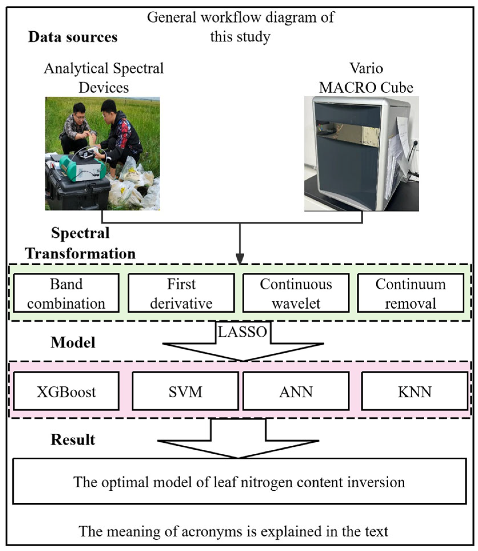
Upon acquiring the spectral data, the initial transformation of reflectance was performed using ViewSpecPro (V5.6) software, followed by the calculation of average reflectance for each sample group of L. chinensis and C. squarrosa, respectively. Additionally, prior to transformation, the spectral reflectance data required smoothing. This study employed the Savitzky–Golay filter [17] for smoothing to mitigate the random signal noise present in the spectra, with the smoothing process executed in MATLAB (version 2022b, the MathWorks, Inc., Natick, MA, USA) software. Utilizing the smoothed spectral data, the spectral responses of four distinct types of parameters to the nitrogen content in L. chinensis and C. squarrosa were analyzed, and the identified sensitive feature parameters were used as input variables for the model. Four modeling techniques (XGBoost, SVM, ANN, and KNN) were employed to develop inversion models for leaf nitrogen content (LNC) in L. chinensis and C. squarrosa from the typical steppe of Inner Mongolia. The overall workflow is illustrated in Figure 2.
As a high-resolution spectrometer, ASD FieldSpec-4 acquires data that reflect subtle differences in spectral features, but the large number of bands also creates new problems in data processing. The correlation between adjacent bands leads to considerable information redundancy, causing the data distribution in high-dimensional space to become sparse and irregular. This can result in issues such as invalidity, overlap, and other related problems with the spectral information. Directly using the full band for parametric inversion can result in unstable performance of the inversion model and increase the time cost. Thus, it is essential to perform dimensionality reduction and transformation on the hyperspectral data to emphasize the spectral characteristics of the features before developing the inversion model.
The approach employed in this research for dimensionality reduction and the transformation of hyperspectral data involves feature selection. This fundamental process focuses on identifying key bands or parameters from both the original and transformed spectra to preserve the spectral characteristics of ground objects. Ultimately, the original spectral curves were processed using four techniques—band combination, derivative transformation (DT), CWT, and CRT—to facilitate the subsequent extraction of feature variables.
Vegetation indices (VI) represent a combination, either linear or nonlinear, of multiple spectral bands, primarily indicating the contrast in reflective properties between vegetation in the visible and near-infrared bands and the soil background. This approach can mitigate or eliminate the effects of background noise on spectral data from grassland vegetation, thereby enhancing the assessment of vegetation structure. In the present study, a total of 22 VI were analyzed (Table 1), comprising 15 two-band VI and 7 three-band VI. These spectral parameters are extensively employed for estimating biochemical metrics of vegetation. The objective of this research was to evaluate the efficacy of these variables in estimating nitrogen content in the predominant vegetation found within the typical steppe of Inner Mongolia.
DT is a commonly used spectral data processing method. Using DT to process and analyze spectral reflectance data can enhance the effective information in the spectrum, highlight the finer information in the spectrum, and contribute to the coupling of information in different frequency bands. The hyperspectral data’s First Derivative Transform (FDT) effectively mitigates soil background noise. To examine the characteristics of spectral differences, the ‘trilateral parameter’ is derived from the inflection point of the derivative spectral curve, as well as from the positions of maximum and minimum reflectance, alongside other pertinent features. Concurrently, the ‘three-edge parameter’ functions as a correlation variable that is contingent upon the positional attributes of the derivative spectrum. The ‘three edges,’ which encompass red, blue, and yellow, pinpoint specific locations within the spectral curve that more accurately represent the spectral characteristics of green vegetation. Notably, parameters related to the red edge exhibit heightened sensitivity to the levels of essential plant nutrients, including nitrogen and chlorophyll. In this study, a total of 19 feature parameters, identified through various spectral positions and areas, have been compiled (Table 2). They were used for subsequent feature screening and modeling to find the best method to monitor the LNC of the two vegetation types.
Wavelet transformation (WT) is a crucial method for signal processing and analysis that builds upon Fourier transform. This technique facilitates the decomposition of a random signal into linear combinations of wavelet basis functions across various scales, thereby enabling a comprehensive time–frequency analysis of the signal [40]. In comparison to the Fourier transform, the wavelet transform provides a more effective representation of a signal’s instantaneous characteristics and has become widely utilized in hyperspectral data processing [41]. Regarding hyperspectral reflectance signals, the wavelet transform proves beneficial for identifying spectral variations by analyzing reflectance information at multiple scales while maintaining the original range and position of the bands [42]. The commonly used wavelet transforms are divided into discrete wavelet transformation (DWT) and CWT. However, when dealing with near-Earth hyperspectral data, the discrete wavelet transform tends to lose some useful information, making it difficult to analyze the output parameters [43]. Therefore, this study adopted CWT to decompose the raw spectra of L. chinensis and C. squarrosa leaves. The results were straightforward to interpret because the wavelet coefficients from each wavelet of the CWT were directly comparable to the input reflectance bands [44]. The calculation is given by the following:
ψ a , b λ = 1 a ψ λ b a
where ψ λ denotes the parent wavelet; ψ a , b λ signifies a series of subsequent wavelets generated through the translation and scaling of the parent wavelet, λ represents the spectral wavelengths ranging from 350 to 2500 nm, and a and b are positive real numbers that correspond to the scaling and translation parameters. The convolution of the initial spectrum with these subsequent wavelets yields the wavelet coefficients W f ( a , b ) , which are also referred to as wavelet features W F b , a .
W f a , b = f , ψ a , b = + f λ ψ a , b λ d λ
where f , ψ a , b signifies the inner product of the original spectrum with the continuous wavelets, and f λ indicates the original reflectance spectrum.
The original spectrum of vegetation must be decomposed at various scales using the wavelet basis function, which generates a series of wavelet coefficients through wavelet transformation. In this research, the second-order derivative of the Gaussian function was employed as the wavelet basis function for the continuous wavelet transform (CWT). Specifically, the mexh wavelet was utilized as the mother wavelet due to its similarity to the features of the vegetation spectral profile [44]. The whole transformation process was implemented in MATLAB (V2022b) software, and nine scaling factors were set, ranging from 21 to 29. Finally, the original spectral transformed wavelet coefficient datasets with different scales were obtained for subsequent analysis and modeling.
The CR method is a technique of spectral analysis that significantly improves the characteristics of absorption. It highlights absorption features in the spectrum by calculating the envelope of the spectrum and removing continuum information from the original spectrum [45]. Following the CRT, the absorption characteristics of the spectral curves become more pronounced, with reflectance standardized to a range of 0 to 1. This adjustment helps diminish background noise and effectively separates spectral absorption traits [46]. The calculation is given by the following:
R i = R i R C i
where R ( i ) represents the spectral reflectance with the continuum removed, R ( i ) denotes the original spectral reflectance, and R C ( i ) refers to the reflectance of the continuum line.
After the CR transformation of the original spectrum 350–2500 nm, three distinct absorption peaks were observed. Therefore, 15 CR transformation feature parameters were extracted for subsequent feature screening and model building based on previous studies (Table 3).

2.3.2. Variable Screening Methods

Hyperspectral data, with their high dimensionality and inter-band correlations, pose challenges for modeling leaf nitrogen content (LNC) in grassland vegetation. The dataset, including 22 vegetation indices (VIs, Table 1), 18 first-order derivative transformation (FDT, Table 2) parameters, 15 CRT parameters (Table 3), and CWT coefficients, requires robust variable screening to reduce multicollinearity and enhance model performance.
In this research, feature parameters were screened using the LASSO method after applying various spectral transformations. The LASSO technique, introduced by Tibshirani, functions as a biased estimation approach to address multicollinearity in data [47]. By formulating a penalty function, LASSO facilitates the development of a refined regression model that can reduce some coefficients to zero without significantly affecting the overall model, thereby enhancing the sparsity of certain feature coefficients. Finally, it automatically selects important features related to the target variables with enhanced interpretability [48]. In this study, the feature variables of VI, hyperspectral feature parameters, wavelet coefficients, and CR parameters were selected by the LASSO method, and the filtered variables were used as input variables for machine learning modeling methods. The LASSO method is implemented in Rstudio (V4.4.1) via the “glmnet” package.

2.3.3. Modeling Algorithms

Regression in machine learning is a supervised technique aimed at forecasting continuous values. To explore the effectiveness of different spectrally transformed feature parameters in monitoring the LNC indexes of gramineous plants L. chinensis and C. squarrosa, various machine learning algorithms were applied. Different types of feature parameters were input into the monitoring model separately. In this study, XGBoost, SVM, ANN, and KNN were employed to develop LNC monitoring models using various spectral transformation feature parameters for L. chinensis and C. squarrosa.
XGBoost is a machine learning model built on the gradient boosting decision tree (GBDT) algorithm, which makes a series of improvements and optimizations based on GBDT, including regularization, approximation optimization, feature splitting strategies, and parallel computing [49]. These improvements give XGBoost certain advantages in training speed, model accuracy, and generalization ability [50].
SVM is a supervised learning model in machine learning, widely applied to classification and regression tasks [51]. When solving the regression problem, only one class of sample points exists in the SVM. Unlike classification problems, the SVM algorithm aims to find the optimal hyperplane by minimizing the total deviation of all sample points from it, rather than focusing on the optimal separation of two or more points [52]. The RBF was selected as the kernel function for the SVM.
ANN serves as a mathematical framework that emulates the processes involved in information transfer and processing, akin to the functioning of neurons in the human brain. Typically, it comprises an input layer, one or more hidden layers, and an output layer, with neurons in each layer interconnected to the respective neurons in the subsequent layer [53]. The model operates on the principle that once the data are introduced, it is processed through multiple neuronal layers and activation functions, ultimately yielding the desired outcomes. Training is performed using the back-propagation algorithm, which progressively fine-tunes the weights and biases that connect neurons, thereby minimizing the discrepancy between its outputs and the actual results [54]. In this investigation, a neural network architecture featuring a single hidden layer was employed.
The KNN regression model was initially introduced by Cover and Hart in 1967 [55]. This model’s fundamental principle is that the target sample’s value is predicted based on its k closest neighboring samples. The mean of the attributes from these k-neighboring samples is attributed to the sample under examination, and the final predicted value is determined by the average output of these k samples [56]. KNN is a theoretically mature quantitative inversion method for remote sensing, with advantages such as comprehensibility, minimal requirement for parameter tuning, and efficient model construction. Meanwhile, it reduces the uncertainty caused by noise, internal variations, and misalignment of sample points.
All procedures were conducted using the R statistical software, specifically employing the ‘tidymodels’ package for dataset partitioning, parameter optimization, and final model execution. Furthermore, five-fold cross-validation was implemented for resampling, and a grid search approach was utilized to refine the hyperparameters of the four modeling techniques, which include “mtry”, “tree_depth”, and “learn_rate” for XGBoost; “cost” and “margin” for SVM, “hidden_units”, “penalty”, and “epochs” for ANN; and “neighbors” and “weight_func” for KNN. Finally, the optimal hyperparameter model for estimating N content in vegetation leaves was determined.

2.4. Model Validation

The performance of the model in estimating the LNC of L. chinensis and C. squarrosa was assessed with the validation sample data. For a comprehensive evaluation of the LNC estimation model, we employed the coefficient of determination (R2), the root mean square error (RMSE), and the mean absolute error (MAE), which are defined as follows:
R 2 = i = 1 n M i M ¯ P i P ¯ i = 1 n M i M ¯ 2 i = 1 n P i P ¯ 2
R M S E = 1 n M i P i 2 n
M A E = 1 n i = 1 n M i P i
where M i is the measured value of LNC, M ¯ is the mean value of the measured LNC, P i is the predicted value based on the LNC prediction model, P ¯ is the mean value of the predicted LNC, and n is the total number of samples.

3. Results and Analyses

3.1. LNC Statistical Analysis of L. chinensis and C. squarrosa

After collecting the leaf reflectance, the LNC was measured using an element analyzer, and 76 observations were obtained for each of the two vegetation types. The descriptive statistics (mean, maximum, minimum, standard deviation, and coefficient of variation) for the LNC changes observed in L. chinensis and C. squarrosa are displayed in Table 4.
As shown in Table 4, the LNC of L. chinensis varies from 1.58% to 3.46%, with a mean of 2.51%, an SD of 0.47, and a coefficient of variation of 18.89%. The LNC of C. squarrosa varies from 0.93% to 2.18%, with a mean of 1.57%, an SD of 0.33, and a coefficient of variation of 21–26%. The mean LNC values of L. chinensis in the training set and test set are 2.51% and 2.49%, the SD are 0.47 and 0.52, and the coefficients of variation are 18.61% and 21.01%, respectively. The mean LNC values of C. squarrosa are 0.93% and 1.09%, the SD are 0.33 and 0.36, and the coefficients of variation are 20.92% and 21.54%, respectively. The validation and test sets are more evenly matched with small differences. The data sets of the validation set and the test set are relatively uniform, with a small difference, which helps to improve the reliability of the model evaluation results.

3.2. Hyperspectral Feature Analysis Under Different Transform Methods

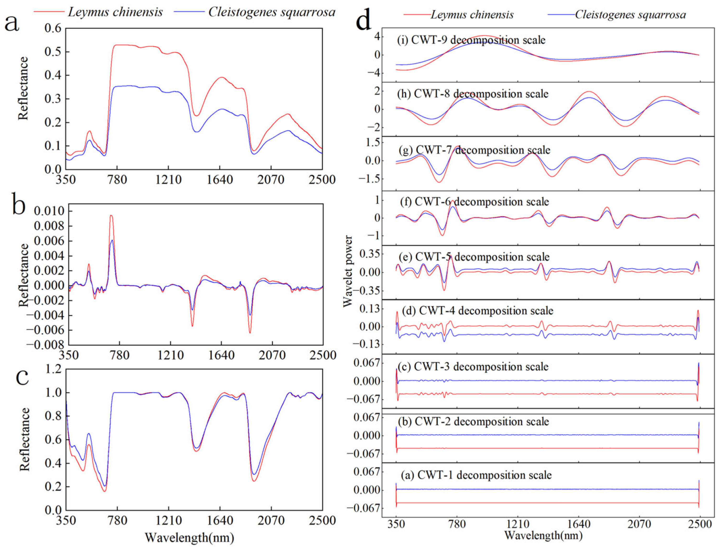
In this study, the original spectral curves were processed through band combination, DT, CWT, and CRT, which scale the absorption and reflection features of the spectra, thus effectively describing the unique spectral information of the terrestrial features. Figure 3 shows the spectra of L. chinensis and C. squarrosa in their original form and after different transformations.
The original spectra of L. chinensis and C. squarrosa leaves are illustrated in Figure 3a. The spectral curves for both species exhibit the characteristic reflectance pattern observed in green vegetation, showing similar peaks and troughs across the spectrum. Notably, L. chinensis generally displays a higher average spectral reflectance than C. squarrosa, particularly in the near-infrared region. Figure 3b presents the spectral curves after the application of the FDT. The curves of the two plants exhibit the same characteristics, both reaching the maximum positive extreme value at a wavelength of about 716 nm. In contrast, the positive extreme value of L. chinensis is greater than that of C. squarrosa, indicating that the reflectance of L. chinensis increases faster in the red edge range.
Figure 3c illustrates the spectral curves for both plants following CR. Within the visible light range (350 to 750 nm) and the near-infrared ranges (1280 to 1680 nm and 1830 to 2220 nm), three absorption valleys are observed. Notably, blue light (350 to 550 nm) and red light (550 to 750 nm) form a “double valley” structure in the spectrum derived from CR.
Figure 3d shows the CWT feature maps at different scales. The wavelet power curves of the two plants are similar overall after the transform, hardly showing distinct plant spectral features at the first to second scales but exhibiting red valley absorption features at the 3rd scale. At the fourth to sixth scales, the wavelet power spectra are relatively flat, with small fluctuation intensities but relatively fast fluctuation frequencies, and show obvious green peaks and red valleys. At the seventh scale, the number of single peaks decreases as the fluctuation frequency decreases, and the manifested detailed features weaken. However, the unique red valley and green peak features of vegetation are still manifested. The wavelet power variation curves at the eighth to ninth scales exhibit a wavy pattern, revealing only the overall features of the plant spectra while losing the detailed features. A comprehensive comparison of the spectral features at the nine scales reveals that the wavelet power spectra at the fourth to sixth scales embody richer information and are more conducive to the discovery and mining of detailed spectral features.

3.3. Correlation Analysis Between Vegetation LNC and Spectral Parameters

3.3.1. Relationship Between L. chinensis LNC and Spectral Variables Under Different Transformations

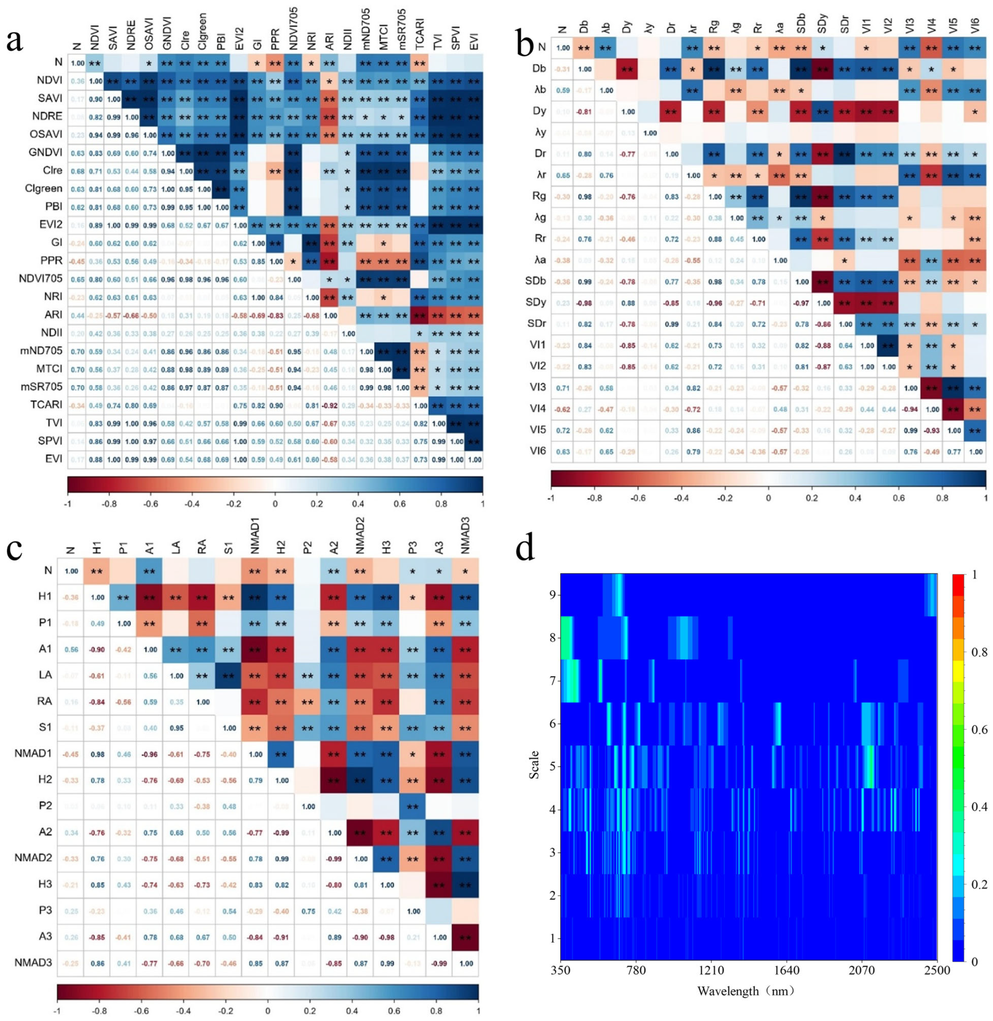
Figure 4 shows the relationship between L. chinensis LNC and spectral variables under different transformations. The correlation coefficients between L. chinensis LNC and VI variables are generally significant, as shown in Figure 4a, and most of them are positive correlations. L. chinensis LNC has good correlations with CIre, mND705, MTCI, mSR705, and TCARI variables ( | R | > 0.7) but weaker correlations with NDVI, SAVI, and NDII ( | R | < 0.1). Among them, LNC shows the greatest positive correlation with MTCI (R = 0.82) and the greatest negative correlation with TCARI (R = −0.87). As shown in Figure 4b, L. chinensis LNC has extremely significant differences with most of the hyperspectral feature variables (p < 0.01), showing good correlations with Db, SDb, SDy, VI3, and VI5 ( | R | > 0.8). The variable with the greatest negative correlation with L. chinensis LNC is SDb (R = −0.87), and the variable with the greatest positive correlation is VI5 (R = 0.84). As shown in Figure 4c, the correlations between L. chinensis LNC and CR parameters are poor compared to those with VI and hyperspectral feature parameters, and most CR variables show weak correlations with LNC ( | R | < 0.2). Only P1, LA, and S1 show extremely significant differences with LNC (p < 0.01), with S1 having the largest correlation (R = −0.50). Figure 4d shows the R2 scales of the correlation analysis between wavelet power and L. chinensis LNC. It can be observed that the effective spectral information of L. chinensis concentrates mainly at the middle scales (third to sixth) after CWT and relatively less at the low scales (first to second) and high scales (seventh to ninth). These results show that the sensitive wavelet feature ranges for the L. chinensis LNC are near 630 nm (third to sixth scales) and near 2044 nm (fourth to sixth scales), and the best wavelet features are WF639,6 (R2 = 0.788) and WF2043,5 (R2 = 0.848), respectively.

3.3.2. Relationships Between C. squarrosa LNC and Spectral Variables Under Different Transformations

Figure 5 shows the relationship between C. squarrosa LNC and spectral variables under different transformations. As shown in Figure 5a, most VI variables show extremely significant differences with C. squarrosa LNC (p < 0.01), and the VI variables with the best correlations are mND705, MTCI, and mSR705, all of which are positive (R = 0.70), which is similar to L. chinensis LNC. In addition, only PPR (R = −0.45) and TCARI (R = −0.34) show good negative correlations. The correlations between the hyperspectral feature variables and the C. squarrosa LNC are shown in Figure 5b. Variables VI3 to VI6, based on the “three-edge” spectral area normalized values and ratios, show good correlations with the C. squarrosa LNC. Among them, variable VI5 has the best positive correlation (R = −0.72), and variable VI4 (R = −0.62) has the best negative correlation. Similar to L. chinensis, C. squarrosa LNC still shows no good correlation with the CR variables, as shown in Figure 5c. The correlation coefficients | R | of most CR variables are below 0.5, with the best positive correlation variable being A1 (R = −0.56) and the best negative correlation variable being NMAD1 (R = −0.45). The coefficient of determination R2 between C. squarrosa LNC and wavelet power is shown in Figure 5d. The areas with better coefficients of determination R2 are mainly concentrated between the third and sixth scales, but the R2 near WF400 nm at the seventh and eighth scales is also good. The best wavelet feature is WF2126,5 (R2 = 0.396).

3.4. LASSO Feature Parameter Screening Results

By employing the LASSO technique, key variables that significantly influence the LNC of L. chinensis and C. squarrosa are identified from the VI variables, hyperspectral feature variables, CR variables, and wavelet coefficient variables. As shown in Table 5, the feature screening process utilizing the LASSO method has notably reduced the number of variables. The screened-out feature variables include those with good correlations with the LNC of the two vegetations. Furthermore, the LAASO feature screening process eliminates variables with zero variance, near-zero variance, and high autocorrelation to avoid errors caused by redundant variables in subsequent modeling.

3.5. LNC Model Construction and Accuracy Evaluation

According to the previous section, four sets of variables were obtained after LASSO feature screening of the LNC of the two grassland vegetations with their spectral variables under different transformations: LASSO-VI variables, LASSO-hyperspectral feature variables, LASSO-CR parameters, and LASSO-wavelet coefficients. To investigate the quantitative regression relationship between the hyperspectral data of L. chinensis and C. squarrosa, along with their leaf nitrogen content (LNC), four distinct sets of variables were utilized as inputs for constructing the XGBoost, SVM, ANN, and KNN models.

3.5.1. L. chinensis LNC Model Construction and Accuracy Evaluation

The four sets of variables obtained through LASSO feature selection were utilized as input parameters for the development of machine learning models designed to estimate leaf nitrogen content in typical grassland vegetation. To identify the optimal model for nitrogen inversion, various estimation models were compared based on their performance metrics. The results of the leaf nitrogen content inversion model for L. chinensis are presented in Table 6.
Table 6 presents the findings of the inversion model for nitrogen content in L. chinensis leaves based on spectral variables. Each model underwent accuracy testing and demonstrated robust performance. For the four models utilizing LASSO-VI variables, the R2 values on the validation set range from 0.65 to 0.74, with RMSE values between 0.26 and 0.30. In contrast, the R2 values for the four models derived from LASSO-hyperspectral feature variables on the validation set span from 0.71 to 0.77, while their corresponding RMSE values range from 0.24 to 0.28. The R2 values for the four models based on the LASSO-CR parameters on the validation set are between 0.55 and 0.77. Additionally, the R2 values for the four models built using LASSO-wavelet coefficients on the validation set range from 0.85 to 0.92, resulting in an improvement in estimation accuracy of approximately 10.4% over inversion models that rely on the other three variable sets. Notably, the multivariate nitrogen content model developed via the SVM algorithm achieved the highest accuracy, accounting for 92% of the variability in nitrogen content. Furthermore, the accuracy disparity between the training and validation sets is approximately 6%, indicating that the model maintains relative stability.
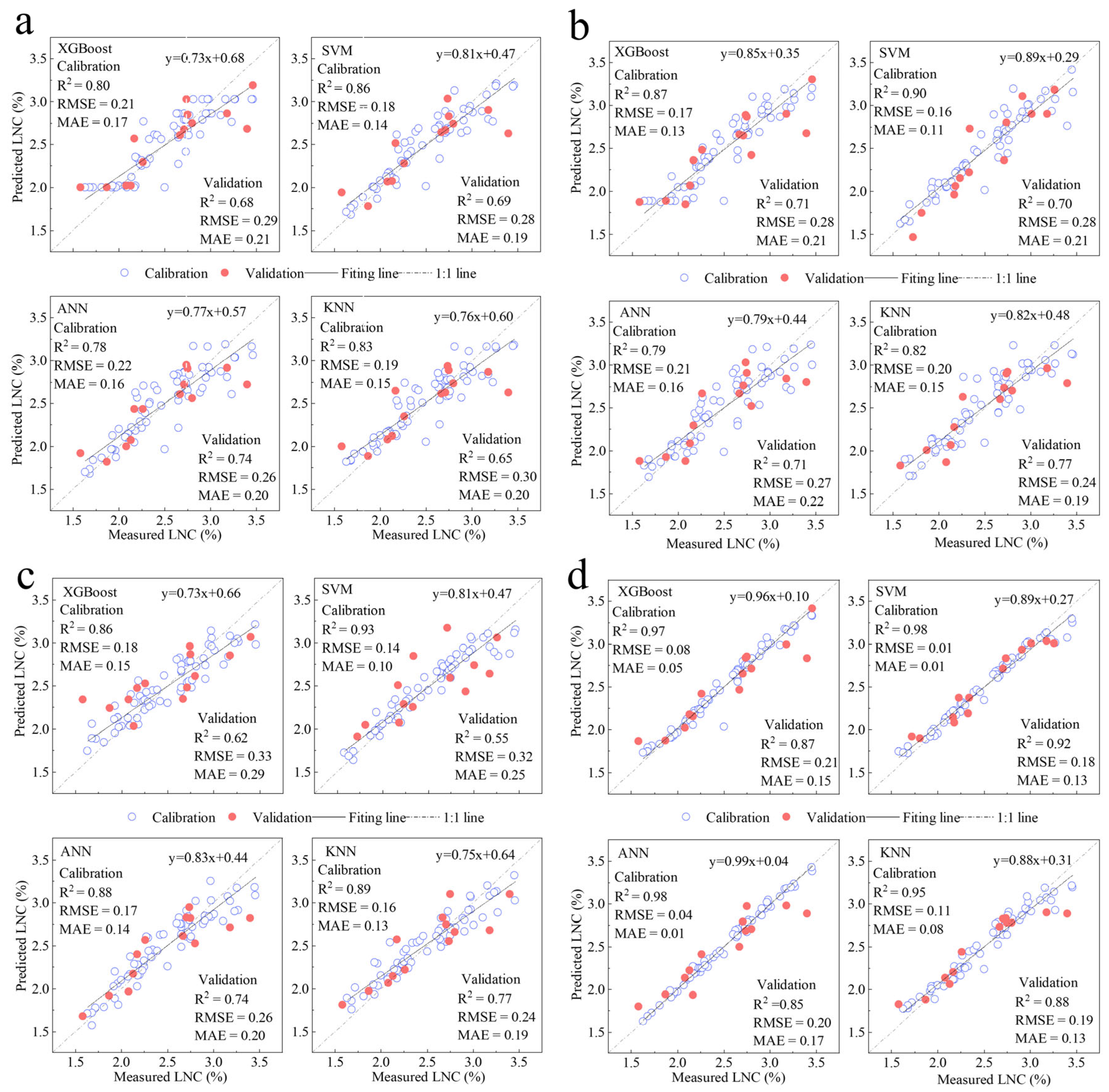
The findings from the inversion models for L. chinensis, developed using four distinct sets of input variables, are presented in Figure 6. The results indicate that the model based on the SVM method demonstrates the highest accuracy, with an R2 value of 0.86, surpassing the models that incorporate VI variables across all four modeling techniques. The R2 values for the remaining three models range from 0.78 to 0.83, suggesting that they also exhibit a satisfactory level of accuracy. However, the model accuracy on the validation set decreases, with the R2 on the validation set between 0.65 and 0.74. Among them, the accuracy of the SVM model decreases by 25%, indicating some overfitting of the model. In comparison, the ANN model is more stable, with an accuracy difference of only 5% on the verification set. In addition, the disparities in RMSE and MAE are also less pronounced, as the predicted and observed points are more uniformly distributed around the fitting line, resulting in improved fitting performance. According to the four nitrogen inversion models constructed based on hyperspectral feature variables and CR parameters, the SVM model has a high model accuracy (R2 of 0.90 to 0.93), but the accuracy on the validation set is poor (R2 of 0.55 to 0.70). Conversely, the ANN and KNN models exhibit greater consistency, achieving higher accuracy on the validation dataset. The inversion models that utilize wavelet coefficient variables demonstrate optimal fitting performance. The nitrogen inversion models constructed using the four machine learning methods have high accuracy, with an R2 between 0.95 and 0.98. Their accuracy on the validation set is good, with the R2 on the validation set between 0.85 and 0.92, indicating that the models are relatively stable. Among the nitrogen inversion models based on wavelet coefficient variables, the SVM model performs the best, explaining 98% of the N content variation in the training set and 92% in the validation set. The RMSE on the validation set is 0.18, and the MAE is 0.13, indicating a superior fit compared to other models.

3.5.2. C. squarrosa LNC Model Construction and Accuracy Evaluation

After LASSO feature screening, four sets of variables were utilized as input to develop models for estimating the leaf nitrogen content of C. squarrosa. The findings are presented in Table 7.
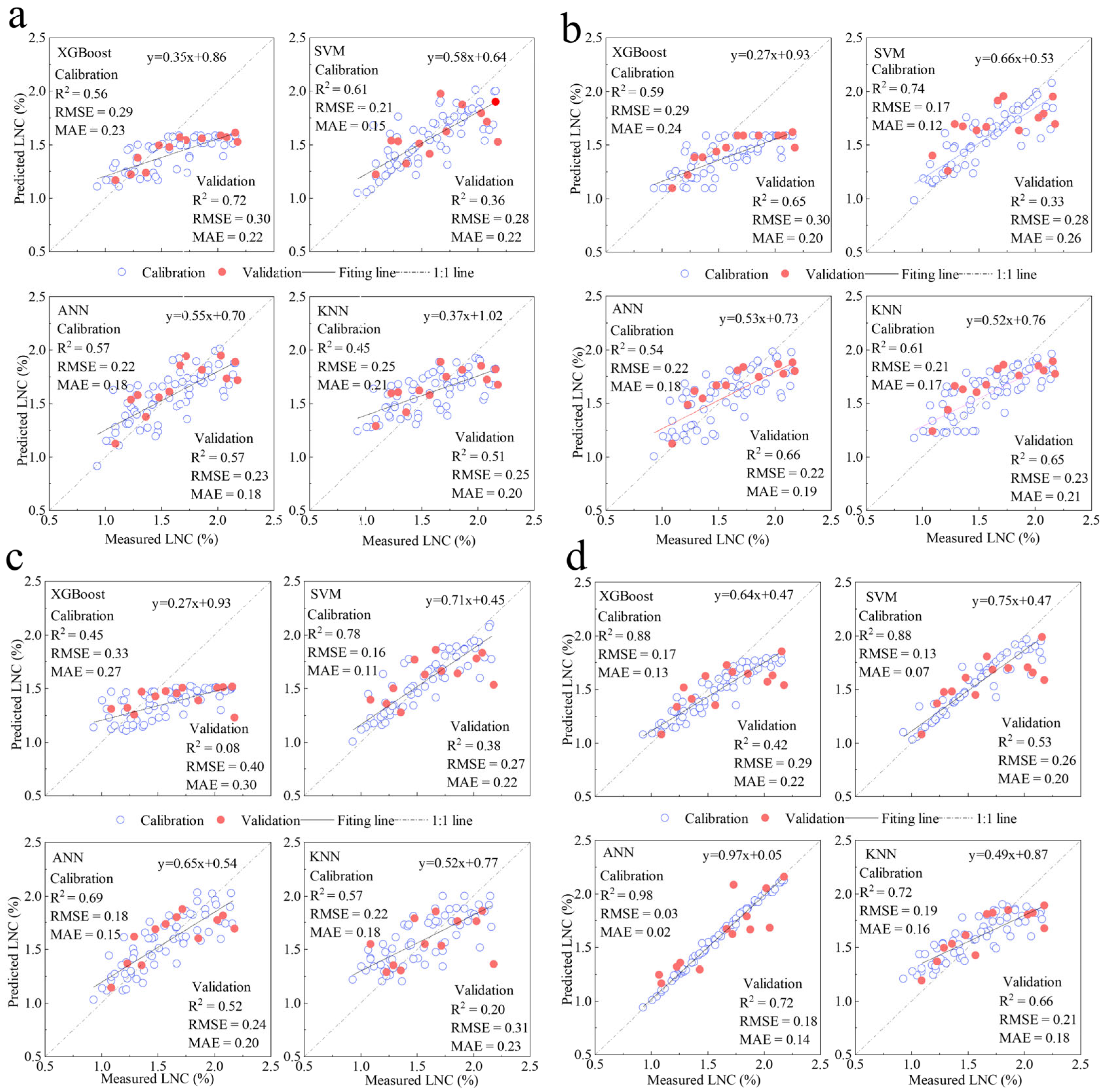
Figure 7 presents the results of the leaf nitrogen content inversion models for C. squarrosa, employing four distinct sets of input variables. The R2 values for the four models utilizing LASSO-VI variables range from 0.45 to 0.61 for the training dataset, while for the validation dataset, they vary between 0.36 and 0.72. In contrast, the inversion models based on LASSO-hyperspectral feature variables and LASSO-CR variables exhibit R2 ranges on the training set of 0.59 to 0.74 and 0.45 to 0.78, respectively. For the validation set, the R2 values for these models range from 0.33 to 0.66 and 0.10 to 0.52, respectively. Overall, the model fitting effects are average, with notable discrepancies between the training and validation sets, indicating a lack of stability. Among the four inversion models utilizing LASSO-wavelet coefficients, the ANN model demonstrates superior estimation performance and achieves the highest accuracy, with an R2 of 0.98 during training and 0.72 during validation. Although there is a slight decrease in accuracy for the ANN model on the validation set compared to the training set, it remains the most precise model overall. Furthermore, the ANN model that incorporates LASSO-wavelet coefficients exhibits greater stability and reliability in comparison to the other models.
Figure 7 presents the outcomes of the leaf nitrogen content inversion models for C. squarrosa, which utilize four distinct sets of input variables. The results indicate that the model developed using the SVM approach achieves the highest accuracy (R2 = 0.61) when compared to the models based on VI variables and the other three modeling techniques. In contrast, the R2 values for the remaining three models range from 0.45 to 0.57. However, the SVM model exhibits lower accuracy on the validation set, with an R2 of only 0.36. In contrast, the XGBoost model has the highest accuracy on the validation set (R2 = 0.72). The ANN model performs similarly on both the training and validation sets, with identical R2 values and only a 0.01 difference in RMSE and MAE, indicating good model stability. However, based on the inversion models constructed with the other three sets of spectral variables, the XGBoost model shows poor fitting. As the nitrogen content increases, the expected values appear to be lower than the actual measurements, leading to data points clustering on the right side of the 1:1 line. While the SVM and KNN models demonstrate superior performance on the training data, their accuracy significantly declines when assessed on the validation data, with the R2 value decreasing by approximately 0.4, indicating a degree of overfitting. In contrast, the ANN model exhibits more consistent performance, showing smaller accuracy variances between the training and validation datasets. Furthermore, the ANN inversion model utilizing LASSO-wavelet coefficients achieves the highest performance, with an R2 of 0.98 in the training dataset and 0.72 in the validation dataset. The predicted and actual points are distributed more uniformly around both sides of the 1:1 line, indicating a more effective fitting result.
These results suggest that using wavelet transform parameters as independent variables for leaf nitrogen content inversion of L. chinensis and C. squarrosa, two typical grassland plants in Inner Mongolia, yields the best estimation results, offering valuable insights for selecting spectral transformation methods and regression models in future monitoring of nitrogen content in grassland vegetation.

4. Discussion

Despite the achievements attained in the inversion process within this study, several limitations persist. The sampling in the region lacks sufficient representativeness, making it difficult to fully capture the vegetation characteristics across all areas of the typical steppes in Inner Mongolia. Furthermore, this study focuses exclusively on leaf nitrogen content, without examining other crucial nutrient elements of the steppe vegetation. This limitation significantly restricts the broader applicability of the research findings in the field of vegetation nutrient analysis.
For future research endeavors, optimization is imperative across multiple dimensions. Firstly, it is essential to expand the collection of steppe vegetation samples from diverse geographical regions and refine the model accordingly. This enhancement will improve the model’s generality and adaptability in accurately inverting the nitrogen content of steppe vegetation within various ecological settings. Secondly, further investigation into the correlations between hyperspectral data and other nutrient elements of steppe vegetation is required. Based on this exploration, a joint inversion model for multiple nutrient elements should be constructed. This model would provide more comprehensive data support for assessing the overall health status of steppe vegetation. Specific research can be embarked upon from the following pivotal perspectives:

4.1. Nitrogen-Sensitive Band Analysis

Currently, the nitrogen concentration in plants can only be estimated indirectly from the spectral data of various plants. This limitation arises because nitrogen does not exhibit distinct spectral signatures within either the visible and near-infrared (VNIR, 400–1200 nm) or the short-wave infrared (SWIR, 1200–2500 nm) spectral regions. Although evidence suggests that the SWIR region may offer a more accurate estimation of nitrogen content, most studies have primarily relied on VNIR-based spectral indices for nitrogen assessment, resulting in limited application of SWIR [57]. VNIR mainly recognizes chlorophyll-related nitrogen, ignoring other foliar biochemical components, such as proteins, which show weak spectral responses in SWIR [58]. Therefore, further research on SWIR is necessary. Exploration in this area has been limited due to traditional and technological constraints [59].
This study utilizes ASD FieldSpec-4 data within the spectral range of 400 to 2500 nm to analyze the spectral characteristics of nitrogen content in typical grassland vegetation in Inner Mongolia. The spectral transformation methods are employed to enhance the fine absorption features of grassland biochemical indices while reducing interference from soil background and atmospheric noise [60]. CRT improves the estimation of grass quality based on spectral data and enhances band depth differences [61]. The CR parameters of L. chinensis and C. squarrosa have the same variables responsive to nitrogen contents (Table 5), namely, P1, A1, RA, and P2. P1, A1, and RA are commonly used VNIR features, while P2 is a variable in the SWIR range, corresponding to the wavelength with the maximum absorption depth at the SWIR absorption peak (1440 nm for L. chinensis and C. squarrosa). Previous studies have also demonstrated that the model based on wavelet coefficients exhibits superior predictive performance, and successive wavelet decomposition can effectively increase data dimensionality, thereby extracting valuable spectral information [62]. As illustrated in Figure 4d and Figure 5d, the effective spectral information of L. chinensis and C. squarrosa after CWT is predominantly concentrated at the third to sixth scales, with a particularly strong response to nitrogen content near 2044 nm. Previous studies identified the sensitive wavelengths for nitrogen absorption as 1020, l510, 1730, 1980, 2060, 2130, 2180, 2240, and 2300 nm, demonstrating that 1510 nm is the only wavelength in the range of 400 to 2500 nm that is directly correlated with nitrogen content [63,64,65]. The findings of this study are largely consistent with those of previous research, with minor discrepancies likely attributable to differences in species types. Existing studies have shown that nitrogen’s response to specific wavelengths remains stable across various spectral transformations, indicating the potential applicability of these methods for estimating nitrogen content in grassland vegetation.

4.2. Screening Parameter Analysis

Hyperspectral data are characterized by a very narrow bandwidth and often contain a substantial amount of redundant information, which can lead to issues such as multicollinearity and high dimensionality [66]. Multicollinearity may exist among hyperspectral feature parameters, and irrelevant or redundant features can negatively impact the model’s predictive performance. While adding more variables may enhance the predictive capabilities of a model, it generally increases model complexity, thereby limiting its practical applicability [67,68]. Therefore, optimizing the selection of variables based on the prediction objective is crucial for achieving a balance between model accuracy, simplicity, and computational efficiency [69]. The crop nitrogen estimation model constructed using the reflectance of all bands is prone to over-fitting, resulting in reduced predictive performance and limited interpretability [70,71]. Some studies on grassland biochemical parameter estimation have overlooked the issue of accuracy saturation caused by variable combinations [48,72].
Previous studies have shown that preprocessing of spectral data can eliminate spectral noise, enhance spectral properties, and improve model accuracy [73]. In this study, the LASSO technique is applied to select feature parameters for modeling. The findings indicate that LASSO significantly reduces the number of feature variables (Table 5), with most sensitive bands located in the red-edge and near-infrared regions. Moreover, the spectral absorption characteristics within the red-edge range exhibit a strong correlation with plant biochemical parameters [68,74]. Specific spectral bands and indices, such as the red-edge slope and red-edge position, demonstrate a strong sensitivity to the biochemical characteristics of plants [75,76]. In the context of two representative grassland species found in Inner Mongolia, the selection process significantly reduces the number of feature variables, resulting in L. chinensis having fewer model feature parameters than C. squarrosa. The penalty factor influences the number of variables selected following LASSO screening; as this factor increases, the number of chosen variables decreases. However, an excessively high penalty factor may also increase model error, which justifies the application of five-fold cross-validation [77]. This method facilitates a balance between model complexity and accuracy, thereby enhancing its effectiveness in monitoring biochemical parameters in grasslands.

4.3. Prediction Model Analysis

Machine learning algorithms demonstrate superior performance in addressing nonlinear and multivariate problems compared to traditional approaches. To identify the most suitable model for estimating leaf nitrogen content in typical grassland vegetation in Inner Mongolia using hyperspectral data, this study compares the predictive capabilities of four machine learning models: XGBoost, SVM, ANN, and KNN models. The findings reveal that the SVM model, which utilizes wavelet coefficients, achieves the highest performance for L. chinensis, whereas the ANN model, also employing wavelet coefficients, performs best for C. squarrosa. Both models utilize wavelet transform-based sensitive parameters as independent variables, enabling accurate nitrogen content inversion. This is attributed to the ability of wavelet transformation to extract subtle spectral features and capture the overall structural characteristics of the spectral data [78,79]. As shown in Table 6 and Table 7, the SVM and ANN models exhibit comparable predictive accuracy for L. chinensis, and the results are within acceptable error margins. For C. squarrosa, however, the SVM model has a lower R2 value on the validation set, while the ANN model has better stability and reliability. The accuracy of our method is comparable to that of state-of-the-art approaches employing similar spectroscopic techniques, albeit in different application scenarios [80,81]. Therefore, the ANN model based on wavelet coefficients offers greater advantages and stronger species generalization abilities for the leaf nitrogen content inversion of typical grassland vegetation communities in Inner Mongolia. These findings provide meaningful references for the scientific and efficient application of nitrogen fertilizers in these regions.

5. Conclusions

  • Different spectral transformations can highlight spectral information. The original spectral curves for the two grassland plants, L. chinensis and C. squarrosa, exhibit similar shapes and align with the spectral reflectance curves typical of green vegetation. After the FDT, the positive extreme value of L. chinensis is greater than that of C. squarrosa at a wavelength of about 716 nm, and the reflectance of L. chinensis in the red-edge range increases at a faster rate. After the CWT, obvious green peaks and red valleys are observed at the fourth to sixth scales, which are conducive to discovering and extracting subtle spectral features. Upon implementing the CRT, three absorption valleys become apparent within the visible and near-infrared wavelength ranges, while a “double-valley” configuration is observed in the blue and red light ranges. Compared to the initial spectral curves, these spectral changes improve the spectral characteristics, expand the spectral data, and facilitate the extraction of spectral features.
  • Dimensionality reduction can effectively prevent data overfitting. Four sets of variables are obtained using the LASSO method: LASSO-VI variables, LASSO-hyperspectral feature variables, LASSO-CR parameters, and LASSO-wavelet coefficients. The number of feature variables after screening is significantly reduced compared to before, and the number of variables of L. chinensis is smaller than that of C. squarrosa. The LASSO-wavelet coefficients decrease the most (with that of L. chinensis decreasing from 19,359 to 59 and that of C. squarrosa decreasing from 19,359 to 63). The screening process eliminates variables that exhibit zero variance, those with near-zero variance, and those that display high autocorrelation. This approach reduces data redundancy during the modeling phase while also decreasing the dimensionality of the hyperspectral data.
  • Among the 16 constructed multivariate nitrogen inversion models utilizing four sets of spectral variables for L. chinensis, the model employing SVM and wavelet coefficients exhibits the highest performance. It achieves an R2 value of 0.98 on the training dataset, with corresponding RMSE and MAE metrics of 0.02 and 0.03, respectively. The validation dataset results in an R2 of 0.92, alongside RMSE and MAE values of 0.18 and 0.13. The approximate 6% accuracy difference between the training and validation datasets indicates the model’s stability and reliability. For the 16 multivariate nitrogen inversion models developed for C. squarrosa using four spectral variable sets, the ANN model based on wavelet coefficients demonstrates superior performance. The training dataset yields an R2 of 0.98, with RMSE and MAE values of 0.03 and 0.02, respectively. However, the validation dataset shows an R2 of 0.72, accompanied by RMSE and MAE values of 0.18 and 0.14. These results provide essential insights for developing a rapid, efficient, and non-destructive estimation model for leaf nitrogen content in typical grassland plant species.
  • Using wavelet transform sensitive parameters as independent variables for leaf nitrogen content inversion of L. chinensis and C. squarrosa, two typical grassland plants in Inner Mongolia, yields the best results, serving as a reference for choosing spectral transformation methods and regression models in future monitoring of nitrogen content in grassland vegetation.

Author Contributions

Writing—original draft preparation, L.J.; writing—review and editing, L.J.; methodology, L.J. and X.W.; resources, L.J. and X.W.; validation, J.D.; software, L.J. and R.W.; data curation, L.J. and R.W.; data curation, H.W.; investigation, Y.S.; investigation, W.W.; investigation, Z.Z.; investigation, C.K. All authors have read and agreed to the published version of the manuscript.

Funding

This research was funded by Basic Research Business Fee Project of Universities Directly under the Inner Mongolia Autonomous Region (JY20220108), the Inner Mongolia Autonomous Region Natural Science Foundation Project (2022LHMS03006), the Inner Mongolia University of Technology Doctoral Research Initiation Fund Project (DC2300001284), the Inner Mongolia Autonomous Region Natural Science Foundation Project (2021MS03082), and the China Scholarship Council Project (202411310006).

Data Availability Statement

The raw data supporting the conclusions of this article will be made available by the authors on request.

Acknowledgments

We acknowledge editors and reviewers for their positive and constructive comments and suggestions and thank the grassland ecology research base of Inner Mongolia University for providing experimental sites.

Conflicts of Interest

The authors declare no conflicts of interest.

Abbreviations

The following abbreviations are used in this manuscript:
NNitrogen
ASDAnalytical Spectral Devices
FDTFirst-order Derivative Transformation
CWTContinuous Wavelet Transformation
CRTContinuum Removal Transformation
LASSOLeast Absolute Shrinkage and Selection Operator
XGBoostExtreme Gradient Boosting
SVMSupport Vector Machine
ANNArtificial Neural Network
KNNK-Nearest Neighbors
CNCCanopy Nitrogen Concentration
LNCLeaf Nitrogen Content
SMLRStepped-Multiple Linear Regression
SVRSupport Vector Regression
GA-ELMGenetic Algorithm–Extreme Learning Machine
VIVegetation Indices
MaxMaximum
MinMinimum
MeanArithmetic Mean
SDStandard Deviation
CVCoefficient of Variation

References

  1. Wang, Z.; Ma, Y.; Zhang, Y.; Shang, J. Review of remote sensing applications in grassland monitoring. Remote Sens. 2022, 14, 2903. [Google Scholar] [CrossRef]
  2. Reinermann, S.; Asam, S.; Kuenzer, C. Remote sensing of grassland production and management—A review. Remote Sens. 2020, 12, 1949. [Google Scholar] [CrossRef]
  3. Yang, X.; Xu, B.; Zhu, X.; Jin, Y.; Li, J.; Zhao, F.; Chen, S.; Guo, J.; Ma, H.; Yu, H. A monitoring indicator system for remote sensing of grassland vegetation growth and suitability evaluation—A case study of the Xilingol Grassland in Inner Mongolia, China. Int. J. Remote Sens. 2015, 36, 5105–5122. [Google Scholar] [CrossRef]
  4. Bangira, T.; Mutanga, O.; Sibanda, M.; Dube, T.; Mabhaudhi, T. Remote Sensing Grassland Productivity Attributes: A Systematic Review. Remote Sens. 2023, 15, 2043. [Google Scholar] [CrossRef]
  5. Riggs, C.E.; Hobbie, S.E.; Bach, E.M.; Hofmockel, K.S.; Kazanski, C.E. Nitrogen addition changes grassland soil organic matter decomposition. Biogeochemistry 2015, 125, 203–219. [Google Scholar] [CrossRef]
  6. He, J.-S.; Wang, L.; Flynn, D.F.; Wang, X.; Ma, W.; Fang, J. Leaf nitrogen: Phosphorus stoichiometry across Chinese grassland biomes. Oecologia 2008, 155, 301–310. [Google Scholar] [CrossRef]
  7. Beeri, O.; Phillips, R.; Hendrickson, J.; Frank, A.B.; Kronberg, S. Estimating forage quantity and quality using aerial hyperspectral imagery for northern mixed-grass prairie. Remote Sens. Environ. 2007, 110, 216–225. [Google Scholar] [CrossRef]
  8. Mutanga, O.; Adam, E.; Adjorlolo, C.; Abdel-Rahman, E.M. Evaluating the robustness of models developed from field spectral data in predicting African grass foliar nitrogen concentration using WorldView-2 image as an independent test dataset. Int. J. Appl. Earth Obs. Geoinf. 2015, 34, 178–187. [Google Scholar] [CrossRef]
  9. Gao, J.; Liang, T.; Yin, J.; Ge, J.; Xie, H. Estimation of Alpine Grassland Forage Nitrogen Coupled with Hyperspectral Characteristics during Different Growth Periods on the Tibetan Plateau. Remote Sens. 2019, 11, 2085. [Google Scholar] [CrossRef]
  10. Poonsak, M.; Wasinee, W. Estimations of Nitrogen Concentration in Sugarcane Using Hyperspectral Imagery. Sustainability 2018, 10, 1266. [Google Scholar] [CrossRef]
  11. Guo, J.; Zhang, J.; Xiong, S.; Zhang, Z.; Wei, Q.; Zhang, W.; Feng, W.; Ma, X. Hyperspectral assessment of leaf nitrogen accumulation for winter wheat using different regression modeling. Precis. Agric. 2021, 22, 1634–1658. [Google Scholar] [CrossRef]
  12. Yu, F.; Feng, S.; Du, W.; Wang, D.; Guo, Z.; Xing, S.; Jin, Z.; Cao, Y.; Xu, T. A study of nitrogen deficiency inversion in rice leaves based on the hyperspectral reflectance differential. Front. Plant Sci. 2020, 11, 573272. [Google Scholar] [CrossRef]
  13. Yang, Z.; Li, Y.; Wang, Y.; Cheng, J.; Li, F.Y. Preferences for different nitrogen forms in three dominant plants in a semi-arid grassland under different grazing intensities. Agric. Ecosyst. Environ. 2022, 333, 107959. [Google Scholar] [CrossRef]
  14. Wu, N.; Liu, G.; Yang, Y.; Song, X.; Bai, H. Dynamic monitoring of net primary productivity and its response to climate factors in native grassland in Inner Mongolia using a light-use efficiency model. Acta Prataculturae Sin. 2020, 29, 1–10. [Google Scholar] [CrossRef]
  15. Wang, R.; Dong, J.; Jin, L.; Sun, Y.; Baoyin, T.; Wang, X. Improving the Accuracy of Vegetation Index Retrieval for Biomass by Combining Ground-UAV Hyperspectral Data—A New Method for Inner Mongolia Typical Grasslands. Phyton 2024, 93, 387–411. [Google Scholar] [CrossRef]
  16. Geng, Q.; Ma, X.; Peng, F.; Zhu, Z.; Li, Q.; Xu, D.; Ruan, H.; Xu, X. Consistent responses of the C:N:P stoichiometry of green leaves and fine roots to N addition in poplar plantations in eastern coastal China. Plant Soil 2023, 485, 377–394. [Google Scholar] [CrossRef]
  17. Savitzky, A.; Golay, M.J. Smoothing and differentiation of data by simplified least squares procedures. Anal. Chem. 1964, 36, 1627–1639. [Google Scholar] [CrossRef]
  18. Tucker, C.J. Red and photographic infrared linear combinations for monitoring vegetation. Remote Sens. Environ. 1979, 8, 127–150. [Google Scholar] [CrossRef]
  19. Huete, A.R. A soil-adjusted vegetation index (SAVI). Remote Sens. Environ. 1988, 25, 295–309. [Google Scholar] [CrossRef]
  20. Barnes, E.; Clarke, T.; Richards, S.; Colaizzi, P.; Haberland, J.; Kostrzewski, M.; Waller, P.; Choi, C.; Riley, E.; Thompson, T. Coincident detection of crop water stress, nitrogen status and canopy density using ground based multispectral data. In Proceedings of the Fifth International Conference on Precision Agriculture, Bloomington, MN, USA, 16–19 July 2000; p. 6. [Google Scholar]
  21. Rondeaux, G.; Steven, M.; Baret, F. Optimization of soil-adjusted vegetation indices. Remote Sens. Environ. 1996, 55, 95–107. [Google Scholar] [CrossRef]
  22. Gitelson, A.A.; Kaufman, Y.J.; Merzlyak, M.N. Use of a green channel in remote sensing of global vegetation from EOS-MODIS. Remote Sens. Environ. 1996, 58, 289–298. [Google Scholar] [CrossRef]
  23. Gitelson, A.A.; Gritz, Y.; Merzlyak, M.N. Relationships between leaf chlorophyll content and spectral reflectance and algorithms for non-destructive chlorophyll assessment in higher plant leaves. J. Plant Physiol. 2003, 160, 271–282. [Google Scholar] [CrossRef]
  24. Rao, N.R.; Garg, P.; Ghosh, S.; Dadhwal, V. Estimation of leaf total chlorophyll and nitrogen concentrations using hyperspectral satellite imagery. J. Agric. Sci. 2008, 146, 65–75. [Google Scholar] [CrossRef]
  25. Jiang, Z.; Huete, A.R.; Didan, K.; Miura, T. Development of a two-band enhanced vegetation index without a blue band. Remote Sens. Environ. 2008, 112, 3833–3845. [Google Scholar] [CrossRef]
  26. Peñuelas, J.; Gamon, J.; Fredeen, A.; Merino, J.; Field, C. Reflectance indices associated with physiological changes in nitrogen-and water-limited sunflower leaves. Remote Sens. Environ. 1994, 48, 135–146. [Google Scholar] [CrossRef]
  27. Gitelson, A.; Merzlyak, M.N. Spectral reflectance changes associated with autumn senescence of Aesculus hippocastanum L. and Acer platanoides L. leaves. Spectral features and relation to chlorophyll estimation. J. Plant Physiol. 1994, 143, 286–292. [Google Scholar] [CrossRef]
  28. Schleicher, T.D.; Bausch, W.C.; Delgado, J.A.; Ayers, P.D. Evaluation and refinement of the nitrogen reflectance index (NRI) for site-specific fertilizer management. In Proceedings of the 2001 ASAE Annual Meeting, Sacramento, CA, USA, 29 July–1 August 2001; p. 1. [Google Scholar]
  29. Gitelson, A.A.; Merzlyak, M.N.; Chivkunova, O.B. Optical properties and nondestructive estimation of anthocyanin content in plant leaves. Photochem. Photobiol. 2001, 74, 38–45. [Google Scholar] [CrossRef]
  30. Hunt, E.R., Jr.; Rock, B.N. Detection of changes in leaf water content using near-and middle-infrared reflectances. Remote Sens. Environ. 1989, 30, 43–54. [Google Scholar] [CrossRef]
  31. Sims, D.A.; Gamon, J.A. Relationships between leaf pigment content and spectral reflectance across a wide range of species, leaf structures and developmental stages. Remote Sens. Environ. 2002, 81, 337–354. [Google Scholar] [CrossRef]
  32. Dash, J.; Curran, P. The MERIS terrestrial chlorophyll index. Int. J. Remote Sens. 2004, 25, 5403–5413. [Google Scholar] [CrossRef]
  33. Haboudane, D.; Miller, J.R.; Tremblay, N.; Zarco-Tejada, P.J.; Dextraze, L. Integrated narrow-band vegetation indices for prediction of crop chlorophyll content for application to precision agriculture. Remote Sens. Environ. 2002, 81, 416–426. [Google Scholar] [CrossRef]
  34. Broge, N.H.; Leblanc, E. Comparing prediction power and stability of broadband and hyperspectral vegetation indices for estimation of green leaf area index and canopy chlorophyll density. Remote Sens. Environ. 2001, 76, 156–172. [Google Scholar] [CrossRef]
  35. Vincini, M.; Frazzi, E.; D’Alessio, P. Angular dependence of maize and sugar beet VIs from directional CHRIS/Proba data. In Proceedings of the 4th ESA CHRIS PROBA Workshop, Piacenza, Italy, 19–21 September 2006; pp. 19–21. [Google Scholar]
  36. Huete, A.; Didan, K.; Miura, T.; Rodriguez, E.P.; Gao, X.; Ferreira, L.G. Overview of the radiometric and biophysical performance of the MODIS vegetation indices. Remote Sens. Environ. 2002, 83, 195–213. [Google Scholar] [CrossRef]
  37. Wang, X.; Xu, G.; Feng, Y.; Peng, J.; Gao, Y.; Li, J.; Han, Z.; Luo, Q.; Ren, H.; You, X. Estimation Model of Rice Aboveground Dry Biomass Based on the Machine Learning and Hyperspectral Characteristic Parameters of the Canopy. Agronomy 2023, 13, 1940. [Google Scholar] [CrossRef]
  38. Li, C.; Chen, P.; Ma, C.; Feng, H.; Wei, F.; Wang, Y.; Shi, J.; Cui, Y. Estimation of potato chlorophyll content using composite hyperspectral index parameters collected by an unmanned aerial vehicle. Int. J. Remote Sens. 2020, 41, 8176–8197. [Google Scholar] [CrossRef]
  39. Kong, B.; Yu, H.; Du, R.; Wang, Q. Quantitative estimation of biomass of alpine grasslands using hyperspectral remote sensing. Rangel. Ecol. Manag. 2019, 72, 336–346. [Google Scholar] [CrossRef]
  40. Zhang, J.; Pu, R.; Loraamm, R.W.; Yang, G.; Wang, J. Comparison between wavelet spectral features and conventional spectral features in detecting yellow rust for winter wheat. Comput. Electron. Agric. 2014, 100, 79–87. [Google Scholar] [CrossRef]
  41. Wang, Z.; Chen, J.; Fan, Y.; Cheng, Y.; Wu, X.; Zhang, J.; Wang, B.; Wang, X.; Yong, T.; Liu, W. Evaluating photosynthetic pigment contents of maize using UVE-PLS based on continuous wavelet transform. Comput. Electron. Agric. 2020, 169, 105160. [Google Scholar] [CrossRef]
  42. Gu, X.; Wang, Y.; Sun, Q.; Yang, G.; Zhang, C. Hyperspectral inversion of soil organic matter content in cultivated land based on wavelet transform. Comput. Electron. Agric. 2019, 167, 105053. [Google Scholar] [CrossRef]
  43. Lin, D.; Li, G.; Zhu, Y.; Liu, H.; Li, L.; Fahad, S.; Zhang, X.; Wei, C.; Jiao, Q. Predicting copper content in chicory leaves using hyperspectral data with continuous wavelet transforms and partial least squares. Comput. Electron. Agric. 2021, 187, 106293. [Google Scholar] [CrossRef]
  44. Zhuang, T.; Zhang, Y.; Li, D.; Schmidhalter, U.; Ata-Ui-Karim, S.T.; Cheng, T.; Liu, X.; Tian, Y.; Zhu, Y.; Cao, W.; et al. Coupling continuous wavelet transform with machine learning to improve water status prediction in winter wheat. Precis. Agric. 2023, 24, 2171–2199. [Google Scholar] [CrossRef]
  45. Zhang, J.; Wang, W.; Qiao, H.; Xu, C.; Guo, J.; Si, H.; Wang, J.; Xiong, S.; Ma, X. Estimation of leaf nitrogen content in winter wheat based on continuum removal and discrete wavelet transform. Int. J. Remote Sens. 2023, 44, 5523–5547. [Google Scholar] [CrossRef]
  46. Huang, Z.; Turner, B.J.; Dury, S.J.; Wallis, I.R.; Foley, W.J. Estimating foliage nitrogen concentration from HYMAP data using continuum removal analysis. Remote Sens. Environ. 2004, 93, 18–29. [Google Scholar] [CrossRef]
  47. Tibshirani, R. Regression shrinkage and selection via the lasso. J. R. Stat. Soc. Ser. B Stat. Methodol. 1996, 58, 267–288. [Google Scholar] [CrossRef]
  48. Gao, J.; Meng, B.; Liang, T.; Feng, Q.; Ge, J.; Yin, J.; Wu, C.; Cui, X.; Hou, M.; Liu, J. Modeling alpine grassland forage phosphorus based on hyperspectral remote sensing and a multi-factor machine learning algorithm in the east of Tibetan Plateau, China. ISPRS J. Photogramm. Remote Sens. 2019, 147, 104–117. [Google Scholar] [CrossRef]
  49. Moghimi, A.; Pourreza, A.; Zuniga-Ramirez, G.; Williams, L.E.; Fidelibus, M.W. A novel machine learning approach to estimate grapevine leaf nitrogen concentration using aerial multispectral imagery. Remote Sens. 2020, 12, 3515. [Google Scholar] [CrossRef]
  50. Sudu, B.; Rong, G.; Guga, S.; Li, K.; Zhi, F.; Guo, Y.; Zhang, J.; Bao, Y. Retrieving SPAD values of summer maize using UAV hyperspectral data based on multiple machine learning algorithm. Remote Sens. 2022, 14, 5407. [Google Scholar] [CrossRef]
  51. Cortes, C.; Vapnik, V. Support-vector networks. Mach. Learn. 1995, 20, 273–297. [Google Scholar] [CrossRef]
  52. Mountrakis, G.; Im, J.; Ogole, C. Support vector machines in remote sensing: A review. ISPRS J. Photogramm. Remote Sens. 2011, 66, 247–259. [Google Scholar] [CrossRef]
  53. Atkinson, P.M.; Tatnall, A.R. Introduction neural networks in remote sensing. Int. J. Remote Sens. 1997, 18, 699–709. [Google Scholar] [CrossRef]
  54. Wang, L.; Chang, Q.; Li, F.; Yan, L.; Huang, Y.; Wang, Q.; Luo, L. Effects of growth stage development on paddy rice leaf area index prediction models. Remote Sens. 2019, 11, 361. [Google Scholar] [CrossRef]
  55. Cover, T.; Hart, P. Nearest neighbor pattern classification. IEEE Trans. Inf. Theory 1967, 13, 21–27. [Google Scholar] [CrossRef]
  56. Liu, X.; Zhang, Z.; Jiang, T.; Li, X.; Li, Y. Evaluation of the effectiveness of multiple machine learning methods in remote sensing quantitative retrieval of suspended matter concentrations: A case study of Nansi Lake in North China. J. Spectrosc. 2021, 2021, 1–17. [Google Scholar] [CrossRef]
  57. Alexander, J.; Hubert, H.; Ellen, A.H.; Andreas, B.; Jens, B.; Georg, B. Investigating the Potential of a Newly Developed UAV-Mounted VNIR/SWIR Imaging System for Monitoring Crop Traits—A Case Study for Winter Wheat. Remote Sens. 2021, 13, 1697. [Google Scholar] [CrossRef]
  58. Stroppiana, D.; Fava, F.; Boschetti, M.; Brivio, P.A. Estimation of Nitrogen Content in Herbaceous Plants Using Hyperspectral Vegetation Indices; Hyperspectral Indices and Image Classifications for Agriculture and Vegetation; CRC Press: Boca Raton, FL, USA, 2019; Volume 2. [Google Scholar]
  59. Clevers, J.G.P.W.; Gitelson, A.A. Remote estimation of crop and grass chlorophyll and nitrogen content using red-edge bands on Sentinel-2 and -3. Int. J. Appl. Earth Obs. Geoinf. 2013, 23, 344–351. [Google Scholar] [CrossRef]
  60. Cho, M.A.; Skidmore, A.K. A new technique for extracting the red edge position from hyperspectral data: The linear extrapolation method. Remote Sens. Environ. 2006, 101, 181–193. [Google Scholar] [CrossRef]
  61. Mutanga, O.; Skidmore, A.K.; Kumar, L.; Ferwerda, J. Estimating tropical pasture quality at canopy level using band depth analysis with continuum removal in the visible domain. Int. J. Remote Sens. 2005, 26, 1093–1108. [Google Scholar] [CrossRef]
  62. Li, X.; Shi, Z.; Bai, T.; Chen, B.; Lv, X.; Zhang, Z.; Zhou, B. A Study on the Estimation Model of Hyperspectral Reflectivity and Leaf Nitrogen Content of Cotton Leaves. IEEE Access 2023, 11, 74228–74238. [Google Scholar] [CrossRef]
  63. Schlerf, M.; Atzberger, C.; Hill, J.; Buddenbaum, H.; Werner, W.; Schuler, G. Retrieval of chlorophyll and nitrogen in Norway spruce (Picea abies L. Karst.) using imaging spectroscopy. Int. J. Appl. Earth Obs. Geoinf. 2010, 12, 17–26. [Google Scholar] [CrossRef]
  64. Skidmore, A.K.; Ferwerda, J.G.; Mutanga, O.; Wieren, S.E.V.; Peel, M.; Grant, R.C.; Prins, H.H.T.; Balcik, F.B.; Venus, V. Forage quality of savannas—Simultaneously mapping foliar protein and polyphenols for trees and grass using hyperspectral imagery. Remote Sens. Environ. 2010, 114, 64–72. [Google Scholar] [CrossRef]
  65. Mutanga, O.; Skidmore, A.K. Red edge shift and biochemical content in grass canopies. Isprs J. Photogramm. Remote Sens. 2007, 62, 34–42. [Google Scholar] [CrossRef]
  66. Yi, Q.X.; Huang, J.F.; Wang, F.M.; Wang, X.Z.; Liu, Z.Y. Monitoring rice nitrogen status using hyperspectral reflectance and artificial neural network. Environ. Sci. Technol. 2007, 41, 6770–6775. [Google Scholar] [CrossRef]
  67. Schwarz, G.E. Estimating the Dimension of a Model. Ann. Stat. 1978, 6, 461–464. [Google Scholar] [CrossRef]
  68. Murray, A.B. Reducing model complexity for explanation and prediction. Geomorphology 2007, 90, 178–191. [Google Scholar] [CrossRef]
  69. Corbier, C.; Ugalde, H.M.R. Robust Estimation of Balanced Simplicity-Accuracy Neural Networks-Based Models. J. Dyn. Syst. Meas. Control 2016, 138, 051001. [Google Scholar] [CrossRef]
  70. Thorp, K.R.; Wang, G.; Bronson, K.F.; Badaruddin, M.; Mon, J. Hyperspectral data mining to identify relevant canopy spectral features for estimating durum wheat growth, nitrogen status, and grain yield. Comput. Electron. Agric. 2017, 136, 1–12. [Google Scholar] [CrossRef]
  71. Fu, Y.; Yang, G.; Li, Z.; Li, H.; Li, Z.; Xu, X.; Song, X.; Zhang, Y.; Duan, D.; Zhao, C.; et al. Progress of hyperspectral data processing and modelling for cereal crop nitrogen monitoring. Comput. Electron. Agric. 2020, 172, 105321. [Google Scholar] [CrossRef]
  72. Peerbhay, M.K. Remote sensing of key grassland nutrients using hyperspectral techniques in KwaZulu-Natal, South Africa. J. Appl. Remote Sens. 2017, 11, 036005. [Google Scholar] [CrossRef]
  73. Hunt, E.R.; Doraiswamy, P.C.; Mcmurtrey, J.E.; Daughtry, C.S.T.; Perry, E.M.; Akhmedov, B. A visible band index for remote sensing leaf chlorophyll content at the canopy scale. Int. J. Appl. Earth Obs. Geoinf. 2013, 21, 103–112. [Google Scholar] [CrossRef]
  74. Clevers, J.G.P.W.; Kooistra, L. Using hyperspectral remote sensing data for retrieving total canopy chlorophyll and nitrogen content. In Proceedings of the 2011 3rd Workshop on Hyperspectral Image and Signal Processing: Evolution in Remote Sensing (WHISPERS), Lisbon, Portugal, 6–9 June 2011. [Google Scholar]
  75. Chakraborty, S.K.; Mahanti, N.K.; Mansuri, S.M.; Tripathi, M.K.; Kotwaliwale, N.; Jayas, D.S. Non-destructive classification and prediction of aflatoxin-B1 concentration in maize kernels using Vis–NIR (400–1000 nm) hyperspectral imaging. J. Food Sci. Technol.-Mysore 2020, 58, 437–450. [Google Scholar] [CrossRef] [PubMed]
  76. Remote sensing of forage nutrients: Combining ecological and spectral absorption feature data. ISPRS J. Photogramm. Remote Sens. 2012, 72, 27–35. [CrossRef]
  77. Cao, C.; Wang, T.; Gao, M.; Li, Y.; Li, D.; Zhang, H. Hyperspectral inversion of nitrogen content in maize leaves based on different dimensionality reduction algorithms. Comput. Electron. Agric. 2021, 190, 106461. [Google Scholar] [CrossRef]
  78. Ma, C.; Zhai, L.; Li, C.; Wang, Y. Hyperspectral Estimation of Nitrogen Content in Different Leaf Positions of Wheat Using Machine Learning Models. Appl. Sci. 2022, 12, 7427. [Google Scholar] [CrossRef]
  79. Cheng, T.; Rivard, B.; Sánchez-Azofeifa, A. Spectroscopic determination of leaf water content using continuous wavelet analysis. Remote Sens. Environ. 2011, 115, 659–670. [Google Scholar] [CrossRef]
  80. Sabzi, S.; Pourdarbani, R.; Rohban, M.H.; García-Mateos, G.; Arribas, J.I. Estimation of nitrogen content in cucumber plant (Cucumis sativus L.) leaves using hyperspectral imaging data with neural network and partial least squares regressions. Chemom. Intell. Lab. Syst. 2021, 217, 104404. [Google Scholar] [CrossRef]
  81. Eshkabilov, S.; Lee, A.; Sun, X.; Lee, C.W.; Simsek, H. Hyperspectral imaging techniques for rapid detection of nutrient content of hydroponically grown lettuce cultivars. Comput. Electron. Agric. 2021, 181, 105968. [Google Scholar] [CrossRef]
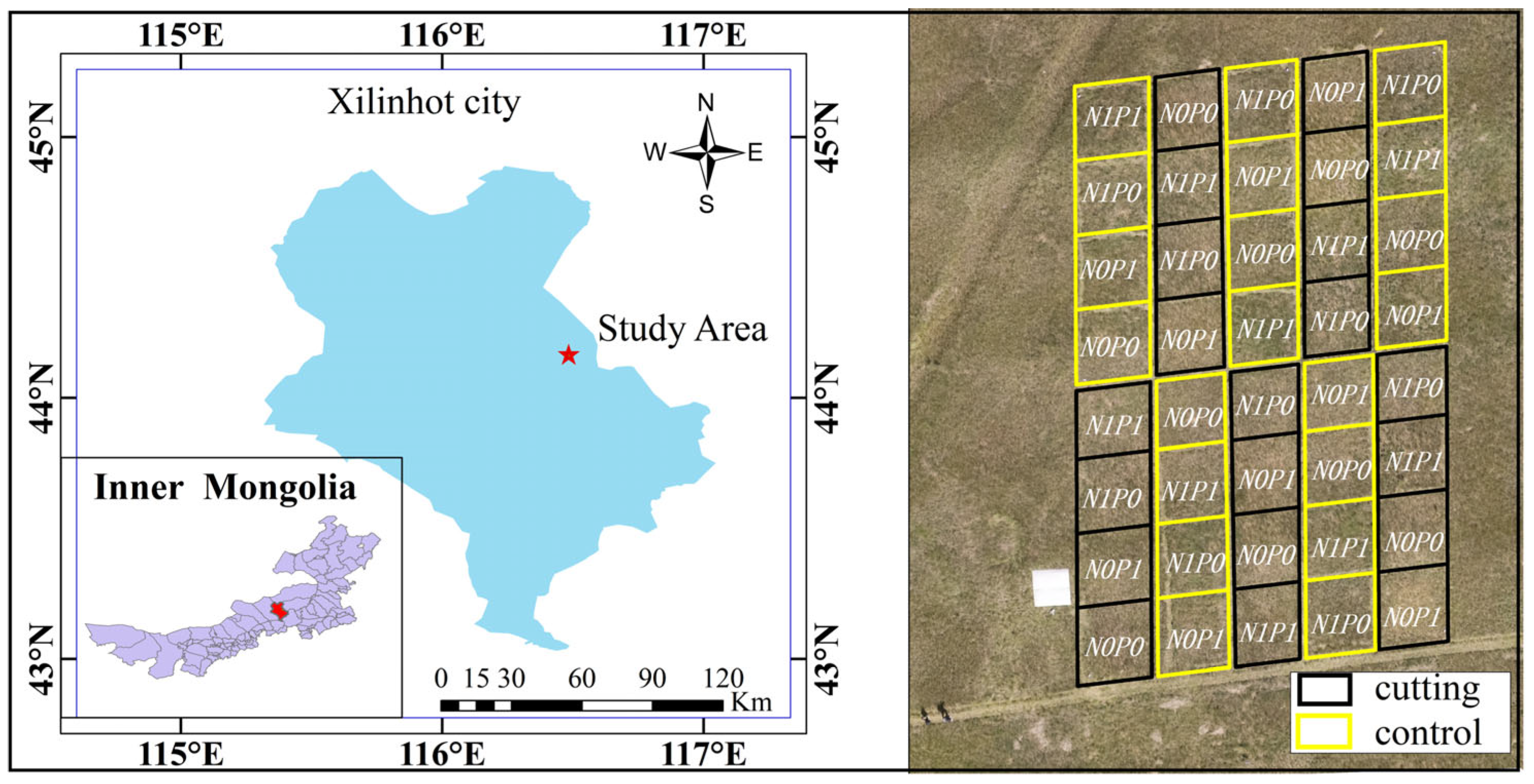
Figure 1. Overview of the study area and sample plot design.
Nitrogen 06 00070 g001
Figure 2. General flow of this study.
Nitrogen 06 00070 g002
Figure 3. Spectra of L. chinensis and C. squarrosa in their original form and after different transformations. (a) Original spectra. (b) FDS. (c) CR spectra. (d) CWT spectra at different scales.
Nitrogen 06 00070 g003
Figure 4. Relationship between L. chinensis LNC and spectral variables under different transformations. (a) Matrix of correlation coefficients between L. chinensis LNC and 22 VI variables. (b) Matrix of correlation coefficients between L. chinensis LNC and 19 hyperspectral feature variables. (c) Matrix of correlation coefficients between L. chinensis LNC and 15 CR variables. (d) Coefficient of determination R2 between L. chinensis LNC and 9 different wavelet power scales.* p < 0.05 and ** p < 0.01.
Nitrogen 06 00070 g004
Figure 5. Relationships between C. squarrosa LNC and spectral variables under different transformations. (a) Matrix of correlation coefficients between C. squarrosa LNC and 22 VI variables. (b) Matrix of correlation coefficients between C. squarrosa LNC and 19 hyperspectral feature variables. (c) Matrix of correlation coefficients between C. squarrosa LNC and 15 CR variables. (d) Coefficient of determination R2 between C. squarrosa LNC and 9 different wavelet power scales. * p < 0.05 and ** p < 0.01.
Nitrogen 06 00070 g005
Figure 6. Scatter plots of the measured values of L. chinensis and the predicted values of the inversion models constructed with the 4 sets of input variables. (a) LASSO-VI variable inversion model of L. chinensis. (b) LASSO-hyperspectral feature parameter inversion model of L. chinensis. (c) LASSO-CR variable inversion model of L. chinensis. (d) LASSO-wavelet power variable inversion model of L. chinensis.
Nitrogen 06 00070 g006
Figure 7. Scatter plots of the measured values of C. squarrosa and the predicted values of the inversion models constructed with the 4 sets of input variables. (a) LASSO-VI variable inversion model of C. squarrosa. (b) LASSO-hyperspectral feature variable inversion model of C. squarrosa. (c) LASSO-CR variable inversion model of C. squarrosa. (d) LASSO-wavelet power variable inversion model of C. squarrosa.
Nitrogen 06 00070 g007
Table 1. The formula for calculating VI and the sources of literature.
NameComputing FormulaReference
Two-band VI
Normalized difference VI (NDVI) ( R 800 R 670 ) / ( R 800 + R 670 ) [18]
Soil adjustment VI (SAVI) 1.5 × ( R 800 R 670 ) / ( R 800 + R 670 + 0.5 ) [19]
Normalized difference red edge index (NDRE) ( R 790 R 720 ) / ( R 790 + R 720 ) [20]
Optimized soil adjusted VI (OSAVI) 1.16 × ( R 800 R 670 ) / ( R 800 + R 670 + 0.16 ) [21]
Green normalized difference VI (GNDVI) ( R 750 R 550 ) / ( R 750 + R 550 ) [22]
Chlorophyll red-edge index (Clre) ( R 750 ) / ( R 720 ) 1 [23]
Chlorophyll greenness index (Clgreen) ( R 800 ) / ( R 560 ) 1 [23]
Plant biochemical index (PBI) ( R 810 ) / ( R 560 ) [24]
Plant pigment ratio (PPR) ( R 550 R 450 ) / ( R 550 + R 450 ) [24]
Two-band enhanced VI (EVI2) 2.5 × ( R 800 R 670 ) / ( R 800 + 2.4 × R 670 + 1 ) [25]
Greenness index (GI) ( R 554 ) / ( R 667 ) [26]
Red-edge normalized difference VI (NDVI705) ( R 750 R 705 ) / ( R 750 + R 705 ) [27]
Nitrogen reflectance index (NRI) ( R 560 R 670 ) / ( R 560 + R 670 ) [28]
Anthocyanin reflectance index (ARI) ( 1 / R 559 ) / ( 1 / R 721 ) [29]
Normalized difference infrared index (NDII) ( R 823 R 1649 ) / ( R 823 + R 1649 ) [30]
Three-band VI
Modified normalized difference index (mND705) ( R 750 R 705 ) / ( R 750 + R 705 2 × R 445 ) [31]
Modified scale VI (mSR705) ( R 750 R 445 ) / ( R 705 R 445 ) [31]
Meris terrestrial chlorophyll index (MTCI) ( R 750 R 710 ) / ( R 710 R 680 ) [32]
Transformed chlorophyll absorption ratio index (TCARI) 3 × R 700 R 670 0.2 × ( R 700 R 550 ) ( R 700 / R 670 ) [33]
Triangular VI (TVI) 0.5 × 120 R 800 R 550 200 × ( R 670 R 550 ) [34]
Spectral polygon VI (SPVI) 0.4 × 3.7 R 800 R 670 1.2 × ( R 530 R 670 ) [35]
Enhanced VI (EVI) 2.5 R 864 R 660 / ( R 864 + 6 × R 660 7.5 × R 487 + 1 ) [36]
Table 2. Hyperspectral feature parameters and extraction methods.
TypeNameDefinition and Calculation MethodReference
Spectral area and positional parametersDbMaximum value of the first-order derivative spectrum within 490–530 nm of the blue edge[37]
λbThe wavelength position corresponding to Db[37]
DyMaximum value of the first-order derivative spectrum within 560–640 nm at the yellow edge[37]
λyThe wavelength position corresponding to Dy[37]
DrMaximum value of the first-order derivative spectrum within 680–760 nm at the red edge[37]
λrThe wavelength position corresponding to Dr[37]
RgGreen peak reflectance, maximum reflectance in the wavelength range of 520–560 nm[37]
λgThe wavelength position corresponding to Rg[38]
RrRed valley reflectance, maximum reflectance in the wavelength range of 650–690 nm[38]
λaThe wavelength position corresponding to Rr[38]
SDbIntegration of FDS in the blue-edge wavelength range of 490–530 nm[38]
SDyIntegration of FDS in the yellow-edge wavelength range of 560–640 nm[38]
SDrIntegration of FDS in the red-edge wavelength range of 680–760 nm[38]
The ratio of spectral area to positional parametersVI1Ratio of green peak reflectance, Rg, to red valley reflectance, Rr[39]
VI2Normalized values of green peak reflectance, Rg, and red valley reflectance, Rr[39]
VI3Ratio of the area of the red side, SDr, to the area of the blue side, SDb[39]
VI4Ratio of the area of the red side, SDr, to the area of the yellow side, SDy[39]
VI5Normalized values for the area of the red edge, SDr, and the area of the blue edge, SDb[39]
VI6Normalized values for the area of the red edge, SDr, and the area of the yellow edge, SDy[39]
Table 3. Definition of CR parameters and extraction method.
NameDefinition
Maximum absorption depth, H1Maximum absorption value in the first absorption peak
Absorption band wavelength, P1Wavelength corresponding to the maximum absorption depth (H) in the first absorption peak
The total area of the absorption peak, A1Integration of the depth of the band within the start and end wavelengths in the first absorption peak
Left area of absorption peak, LAIntegral area of the left absorption peak in the first absorption peak
The right area of absorption peak, RAIntegral area of the right absorption peak in the first absorption peak
Symmetry, S1Ratio of left area (LA) to right area (RA) in the first absorption peak
Maximum absorption depth for area normalization, NMAD1Ratio of the maximum depth of absorption of the first absorption peak (H1) to the total area of the absorption peak (A1)
Maximum absorption depth, H2Maximum absorption value in the second absorption peak
Absorption band wavelength, P2Wavelength corresponding to the maximum absorption depth (H) in the second absorption peak
Total area of absorption peak, A2Integration of the depth of the band within the start and end wavelengths in the second absorption peak
Maximum absorption depth for area normalization, NMAD2Ratio of the maximum depth of absorption of the second absorption peak (H1) to the total area of the absorption peak (A1)
Maximum absorption depth, H3Maximum absorption value in the third absorption peak
Absorption band wavelength, P3Wavelength corresponding to the maximum absorption depth (H) in the third absorption peak
Total area of absorption peak, A3Integration of band depths within the start and end wavelengths in the third absorption peak
Maximum absorption depth for area normalization, NMAD3Ratio of the maximum depth of absorption of the third absorption peak (H1) to the total area of the absorption peak (A1)
Table 4. Statistical description of the LNC (%) of L. chinensis and C. squarrosa.
VegetationDataSample SizeMaxMinMeanSDCV
L. chinensisTotal763.461.582.510.4718.89
Training set633.461.632.510.4718.61
Test set133.41.582.490.5221.01
C. squarrosaTotal762.180.931.570.3321.26
Training set632.160.931.560.3320.92
Test set132.181.091.660.3621.54
Table 5. The LASSO screening results of VI variables, hyperspectral feature variables, and CR variables of the LNC of the two vegetations.
VegetationType of Spectral VariableNumber of VariablesVariable
L. chinensisVI variable2mND705, TCARI
Hyperspectral feature variable3λr, SDy, VI3
CR variable6P1, A1, RA, S1, P2, A2
Wavelet coefficient variable59Scale1: WF528, WF595, WF602, WF622, WF625, WF710;
Scale2: WF596, WF611, WF631, WF642, WF662, WF670, WF709, WF760, WF1096, WF1109, WF1759, WF2240;
Scale3: WF630, WF642, WF2222, WF2239, WF2251;
Scale4: WF594, WF611, WF759, WF851, WF1483, WF1544, WF1626, WF1690, WF2189, WF2238, WF2300, WF2319;
Scale5: WF772, WF1227, WF1692, WF2091, WF2144;
Scale6: WF350, WF631, WF1147, WF1298, WF1609, WF1800, WF2171, WF2254;
Scale7: WF579, WF724, WF1710, WF2337;
Scale8: WF386, WF1039, WF1149;
Scale9: WF773. WF1852, WF2269, WF2500;
C. squarrosaVI variable4mND705, PPR, ARI, NDII
Hyperspectral feature variable4 λ b ,   λ r, VI4, VI6
CR variable7P1, A1, RA, S1, P2, NMAD2, P3
Wavelet coefficient variable63Scale1: WF351, WF666, WF676, WF687, WF688, WF690;
Scale2: WF350, WF508, WF524, WF642, WF689, WF719, WF720, WF1137, WF1146, WF2302;
Scale3: WF522, WF642, WF1146, WF1168;
Scale4: WF368, WF680, WF954, WF1145, WF1540, WF2241, WF2361, WF2381;
Scale5: WF522, WF770, WF1311, WF1566, WF1692, WF1761, WF2127;
Scale6: WF363, WF514, WF631, WF905, WF964, WF1141, WF1259, WF1394, WF1489, WF1708, WF2166, WF2259, WF2486;
Scale7: WF579, WF727, WF1062, WF1380, WF2296;
Scale8: WF406, WF733, WF1084, WF1309, WF2118, WF2412;
Scale9: WF700, WF1329, WF2085, WF2482;
Table 6. Results of the leaf nitrogen content inversion model of L. chinensis with 4 sets of input variables.
Input VariableModelT-R2T-RMSET-MAEV-R2V-RMSEV-MAE
LASSO-VI variableXGBoost0.800.210.170.680.290.21
SVM0.860.180.140.690.280.19
ANN0.780.220.160.740.260.20
KNN0.830.190.150.650.300.20
LASSO-hyperspectral feature variableXGBoost0.870.170.130.710.280.21
SVM0.900.160.110.700.280.21
ANN0.790.210.160.710.270.22
KNN0.820.200.150.770.240.19
LASSO-CR parameterXGBoost0.860.180.150.620.330.29
SVM0.930.140.100.550.320.28
ANN0.880.170.140.740.260.20
KNN0.890.170.130.770.240.19
LASSO-wavelet coefficientXGBoost0.970.080.050.870.210.15
SVM0.980.020.030.920.180.13
ANN0.980.040.030.850.200.17
KNN0.950.110.080.880.190.13
Note: T is the test set (n = 63), and V is the validation set (n = 13).
Table 7. Results of the leaf nitrogen content inversion models of C. squarrosa with 4 sets of input variables.
Input VariableModelT-R2T-RMSET-MAEV-R2V-RMSEV-MAE
LASSO-VIvariableXGBoost0.560.290.230.720.300.22
SVM0.610.210.150.360.280.22
ANN0.570.220.180.570.230.18
KNN0.450.250.210.510.250.20
LASSO-hyperspectral feature variableXGBoost0.590.290.240.650.300.20
SVM0.740.170.120.330.280.26
ANN0.540.220.180.660.220.19
KNN0.610.210.170.650.230.21
LASSO-CR parameterXGBoost0.450.330.270.100.390.30
SVM0.780.160.110.380.270.22
ANN0.690.180.150.520.240.20
KNN0.570.220.180.200.310.23
LASSO-wavelet coefficientXGBoost0.880.170.130.290.420.22
SVM0.870.130.070.260.530.20
ANN0.980.030.020.720.180.14
KNN0.720.190.160.210.660.18
Note: T is the training set (n = 63), and V is the validation set (n = 13).
Disclaimer/Publisher’s Note: The statements, opinions and data contained in all publications are solely those of the individual author(s) and contributor(s) and not of MDPI and/or the editor(s). MDPI and/or the editor(s) disclaim responsibility for any injury to people or property resulting from any ideas, methods, instructions or products referred to in the content.