Systematic Comparison of Sensor Signals for Pump Operating Points Estimation Using Convolutional Neural Network ^†

Abstract

The head and flow rate of a pump characterize the pump performance, which help determine whether maintenance is needed. In the proposed method, instead of a traditional flowmeter and manometer, the operating points are identified using data collected from accelerometers and microphones. The dataset is created from a test rig consisting of a standard centrifugal water pump and measurement system. After implementing preprocessing techniques and Convolutional Neural Networks (CNNs), the trained models are obtained and evaluated. The influence of the sensor location and the performance of different signals or signal combinations are investigated. The proposed method achieves a mean relative error of 7.23% for flow rate and 2.37% for head with the best model. By employing two data augmentation techniques, performance is further improved, resulting in a mean relative error of 3.55% for flow rate and 1.35% for head with the sliding window technique.

1. Introduction

Nowadays, pumping units are installed in many plants for a wide variety of applications. Due to the long operating time, wear and tear such as erosion, abrasion and corrosion are inevitable. The monitoring of operating points and a subsequent evaluation of the condition of the pump may support the decision for required maintenance. Traditionally, flowmeter and manometers are used to determine the operating point of the pump. The installation of these sensors needs to be determined at the beginning of the pipe design—a later installation will be more complicated and troublesome. While an accelerometer and microphone are very flexible, an accelerometer is fixed on the desired surface magnetically, a microphone is fixed by a bracket. The type, position and number of sensors can be easily changed at any time. The idea is to use collected data from those flexible sensors to estimate the operating point of the pump. The next phase of the project aims to extend the method to explore the possibility of using the model trained on one pump to predict the operating state of another pump. In addition, the use of accelerometers and microphones will have the added benefit of being implemented for tasks such as fault identification, cavitation detection, etc., where the conclusions cannot be obtained directly from flow and pressure measurements.

In recent years, convolutional neural networks (CNNs) have attracted widespread attention and obtained huge success in various tasks, such as image recognition and nature language processing. Neural networks have the extraordinary ability of automatic feature extraction. More importantly, expert experience or background knowledge is not necessary for this learning process. Monitoring pump operating point intelligently with CNNs can improve the operation safety, and reduce unnecessary maintenance and personal cost.

Several researchers have applied this powerful tool into the field of hydraulic machinery. ALTobi et al. implemented a Multilayer Feedforward Perceptron Neural Network (MLP) and Support Vector Machine (SVM) to realize the fault condition classification with vibration signal [1]. The faults on the pump were created with a specifically designed test rig. The classification rate reached 99.5% and 98.8%. He et al. combined CNN and a long short-term memory (LSTM) network to conduct the classification of gradually changing faults, reaching an accuracy of 98.4% [2]. Tang et al. proposed a fault diagnosis method for axial piston pumps using a CNN model. The raw vibration signal is converted into images through continuous wavelet transformation [3]. The classification accuracy for five fault types on the test set achieved 96% in 10 trials. Zhao et al. developed an unsupervised self-learning method for the fault diagnosis of centrifugal pumps [4]. Stacked denoising autoencoder (SDA) is implemented to extract features from non-stationary vibration. Wu and Zhang use CNN to identify stall flow patterns in pump turbines [5]. The prediction of stall flow in blade channels achieved an accuracy of 100%, which outperforms existing methods. Look et al. built Auxiliary Classifier Generative Adversarial Networks to detect the occurrence of cavitation in hydraulic machinery, reaching an accuracy of 95.1% for a binary classification [6]. With modified objective function using additional I-divergence, the accuracy was further improved to 98.1%. Cavitation is a common phenomenon in hydraulic machinery, leading to damage of components and a loss of efficiency. Since visual inspection is in many cases not possible, acoustic emissions are used as an alternative to analyze the degree of cavitation erosion (Look et al., 2019) [7]. Harsch et al. implemented an anomaly detection neural network to estimate the cavitation erosion damage using acoustic emissions [8]. Sha et al. proposed a multi-task learning framework with a 1-D double hierarchical residual network [9]. Using an emitted acoustic signal, this network achieves cavitation detection and cavitation intensity recognition at the same time. Besides, the influence of the sampling rate is investigated. Harsch and Riedelbauch proposed a graph neural network model to directly predict the final steady state velocity and pressure fields [10]. The method works well for different systems and does not need a priori domain information. Inspired by those successful applications, the feasibility of the operating point estimation of pumps with CNN is investigated. Gaisser et al. introduced a general-purpose framework to analyze the acoustic emissions of various hydraulic machineries for cavitation detection [11]. The unique advantage of the system is its exclusive training with data from model turbines operated in laboratory settings, enabling it to be directly applied to different prototype turbines in hydro-power plants.

Inspired by the various successful applications of neural networks in the field of hydraulic machinery, we choose the prediction of operating point as an initial goal. Moreover, it is meaningful to compare the input signals in order to know which positions contain more valuable information related to the operating state. High-quality input signal is the basis for subsequent extension to more applications.

There are four main sections, including the introduction. In the second section, the dataset including the details of the test rig and measurement conditions are introduced. Additionally, the preprocessing of raw data, network structure and two data augmentation methods are presented. The third section presents the experiment setup of neural network training, evaluation metrics and the analysis of the results. The fourth section outlines the conclusion and the outlook for further research. This manuscript is an extended version of the ETC2023-160 meeting paper published in the Proceedings of the 15th European Turbomachinery Conference, Budapest, Hungary, 24–28 April 2023 [12].

2. Methods

2.1. Dataset

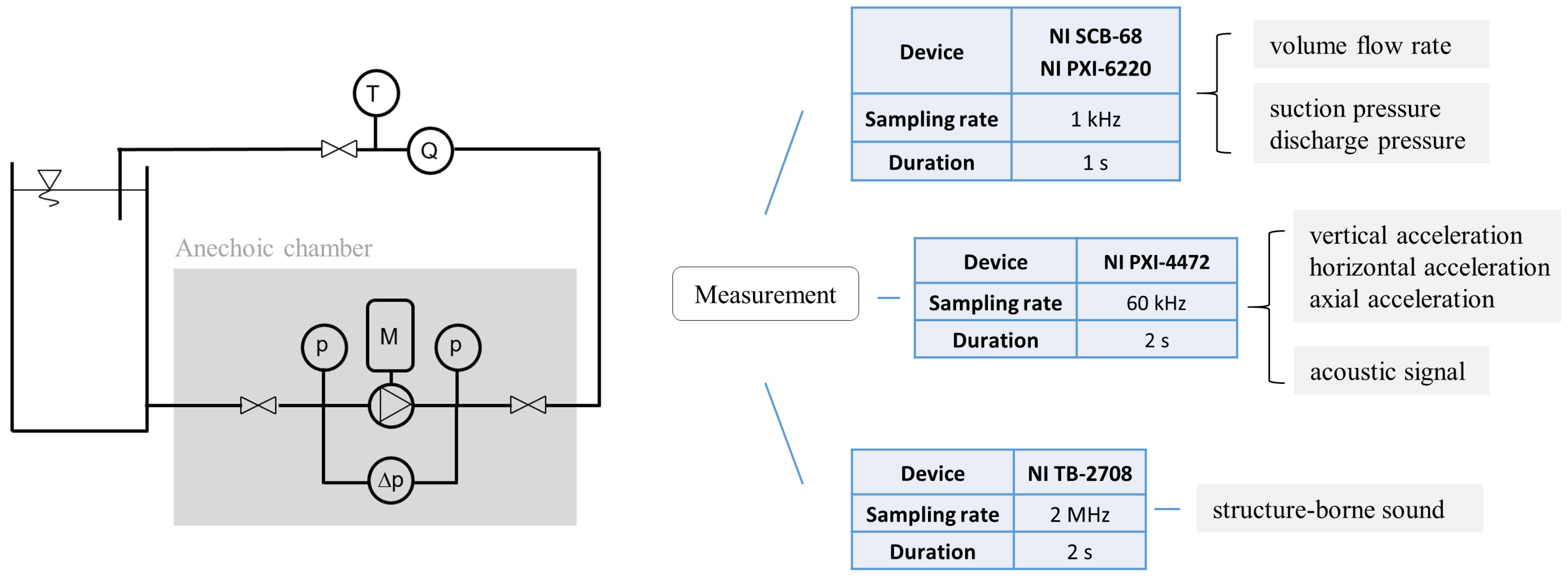
Data are collected on the test bench shown in Figure 1. The pump unit is located in an anechoic chamber, guaranteeing that the microphones only measure the sound of the pump unit. The base is isolated from the metallic grid at the bottom by a rubber pad. A thermometer, flowmeter and manometers are installed on the pipeline. To verify the feasibility of the method, a relatively pure signal obtained from a well-isolated environment is firstly used. In real industrial scenarios, there is inevitably some noise and the vibration brought from other facilities. How the signal with noise will affect the prediction result is to be analyzed and discussed in the next stage of the project.

In the experiments, standard water pumps feature a specific speed $n_q=15.6$ with an impeller diameter of 209 mm. The specific speed is defined as:

$$n_q=n\frac{\sqrt{Q}}{H^{\frac{3}{4}}},$$

(1)

where n is rotational speed (r/min), Q is flow rate (m³/s) at the point of best efficiency and H is head (m) at the point of best efficiency.

A frequency converter is used for speed regulation of the pump. Data are measured under six rotational speeds: 500, 950, 1160, 1500, 2100, 2400 r/min. When measuring individual speeds, the valve opening is step-by-step adjusted to ensure that the pump unit operates along its performance characteristics at different operating points. All measurements are carried out without the presence of cavitation. Flow rate and pressure at suction side and pressure side are collected. The head, a parameter not directly measurable, is calculated as follows:

$$H=\frac{p_p-p_s}{\rho g}+\frac{1}{2g}({(\frac{Q}{A_p})}^2-{(\frac{Q}{A_s})}^2)+h,$$

(2)

where $p_{p/s}$ is the static pressure at pressure side or suction side, $A_p$ and $A_s$ are corresponding pipe cross-section areas, h is the height difference between the pressure sensors on both sides. The measured flow rate and calculated head are fed into the neural network during the training process as the target value.

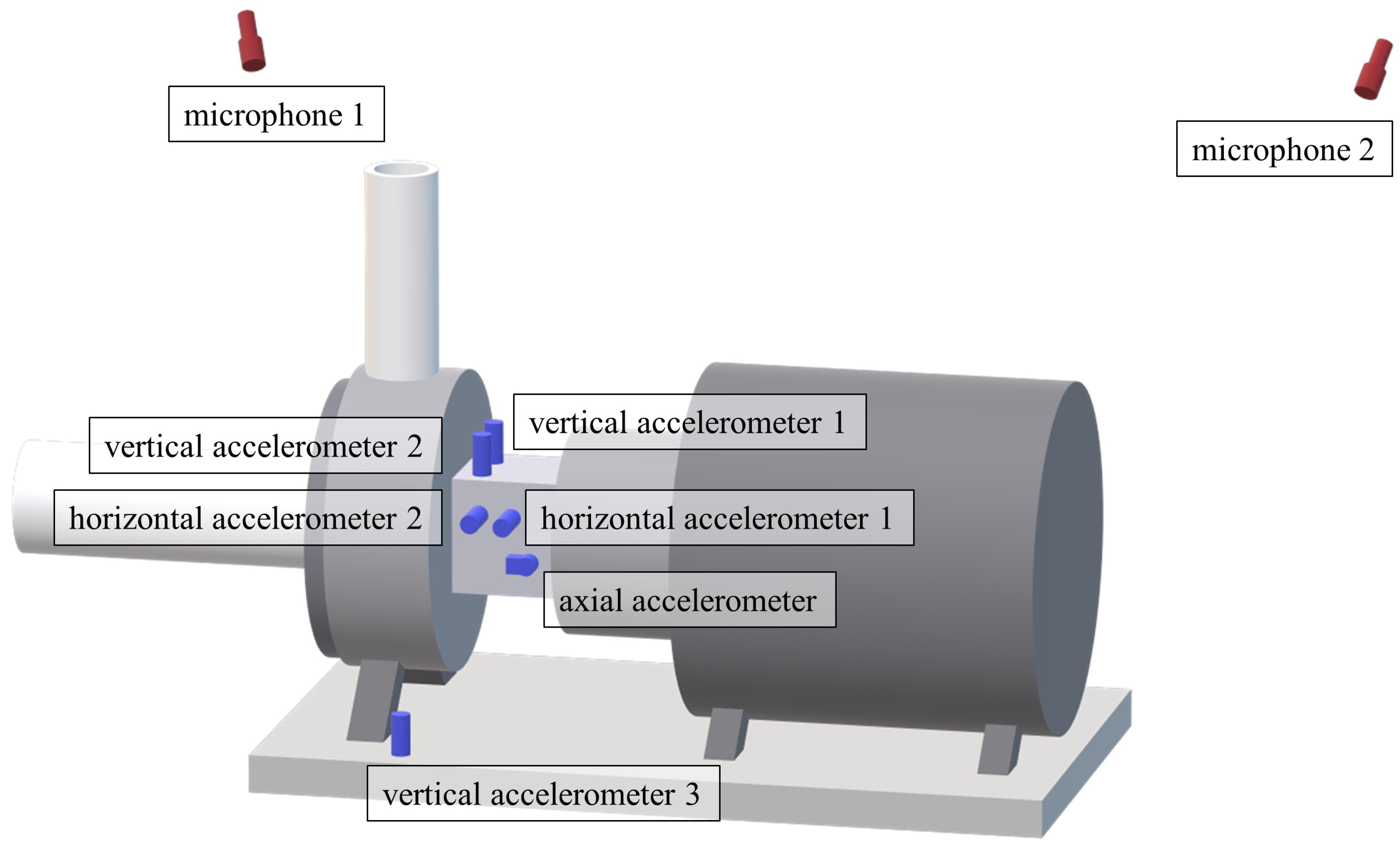
Six accelerometers (Type KS74C and KS80D) are magnetically fixed on the surface of the bearing house and base using a supplied holding magnet. The frequency range of the KS74C type is 0.13–16 kHz, and the frequency range of the KS80D type is 0.13–22 kHz. Vertical accelerometers measure the vibration parallel to the axis of the pressure pipe, while the axial accelerometer measures the vibration parallel to the axis of the suction pipe. The measurement locations and directions are chosen based on the standard ISO 10816-7:2009. Two microphones (Type MM210) with a frequency range from 3.5 Hz to 20 kHz are hung at both sides of the pump unit. The distance from microphone 1 to the pump is 1 m; the distance from microphone 2 to the motor is 0.3 m. These locations are chosen to ensure that the main sources of the microphones are the pump and the motor, respectively. Devices, sampling rate, duration of the measurement and the locations of the sensors are shown in Figure 1 and Figure 2.

2.2. Preprocessing

Instead of processing raw signals, including a huge amount of data points, convolutional neural networks are better suited and more adept at handling image inputs. Hence, the idea of preprocessing is to convert one-dimensional time signals into two-dimensional representations, Figure 3. The middle part of the raw signal is trimmed to a length of one second. After performing standardization, the data has a mean value of zero and a unit standard deviation. Standardization is a re-scale operation that means subtracting the mean and dividing by the standard deviation. Note that the values do not have a bounding range now.

As a powerful time frequency analysis method, Short Time Fourier transform is adopted to realize the transformation. The signal is divided into parts of equal length, and a Fourier transform of each segment is separately computed. Therefore, the spectrogram includes time and frequency information. Tukey windows of length 256 are implemented with a shape parameter of 0.25 and 50% overlap. Based on the results of pre-experiments, converting the linear frequency axis of the spectrogram into a logarithm axis, i.e., Log-Spectrogram, improves the performance of the network.

Although the duration of each signal is one second, the aspect ratio of the resulting spectrogram varies due to different choices of sampling rate and window length. To make it easier for possible subsequent multi-signal combinations and data augmentation, the spectrogram of signals collected from various devices is uniformly resized to 224 × 224. Before being fed into the neural network, the data are normalized into the range $[0, 1]$ and repeated three times in the first dimension.

2.3. Network Structure

To construct a typical CNN, there are three essential building elements in general: a convolutional layer, pooling layer and fully connected layer [13]. The convolutional layer consists of lots of filters, each of that being a group of parameters. During the training process, those parameters are trained to accomplish feature extraction. The pooling layer is used for dimension reduction; max pooling and average pooling are both commonly used non-linear functions. The max or the mean value of the specific region is calculated to represent this area. To realize the classification or regression tasks, the fully connected layer is usually implemented as the last part of the neural network. It builds connections between all neurons in the current layer and previous layer.

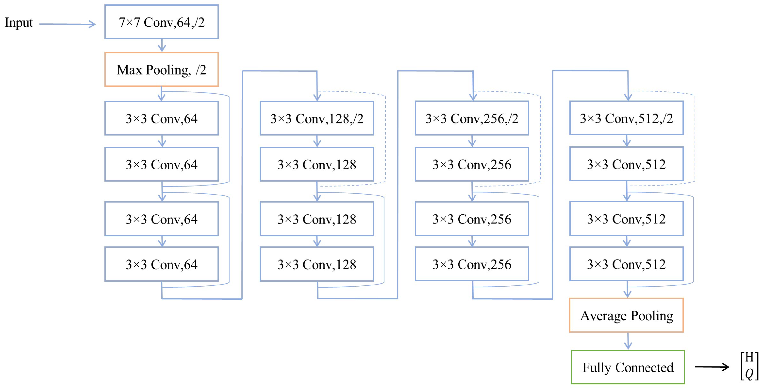
The residual nets (ResNets) are a special variation of CNN. He et al. proposed a framework with residual blocks to solve a degradation problem in deep neural networks [14], Figure 4. The first convolutional layer consists of 64 filters with the shape 3 × 3. The stride is 2, which shrinks the image to half its previous size. After that follows 8 residual convolutional blocks. The difference between the residual block and plain convolutional block is the “skip connection”, which means the input of the block is added to the output of the block. It is represented by the grey line located on the side. A dashed line means the size needs to be halved, because in the corresponding block, the stride for one layer is 2. A non-dashed line means keeping the original size. Different from the original network, the output dimension of the fully connected layer is modified to two. The final output of the network is a 2-dimensional vector, representing head and flow rate.

2.4. Data Augmentation

When training a network with a small dataset, overfitting is always a problem. That is, the network shows good performance on the train set, while on the test set, the result is significantly worse. Mismatch between dataset size and trainable parameter number lead the network to “memorize” the data instead of learning the features. To obtain a network with good generalization, a huge amount of data containing variations is necessary. However, receiving such large amounts of data is unrealistic due to the economic cost and time required. Hence, applying augmentation methods on the available train set with limited data is often essential.

• Sliding Window & Horizontal Flip

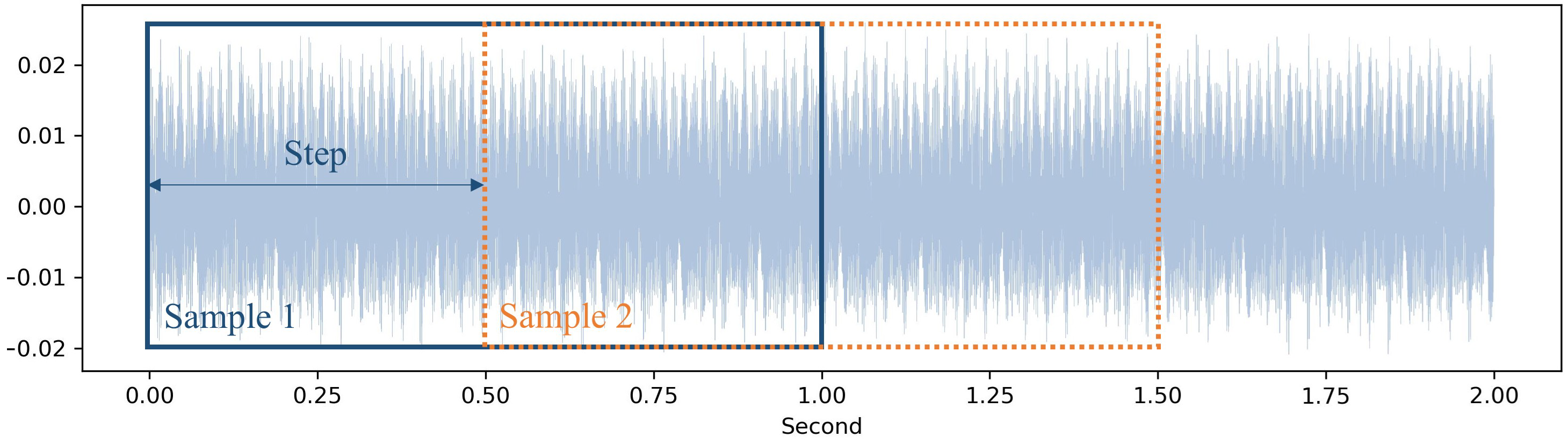
The sliding window method is an effective way to extend the dataset with factor $n_a$, Figure 5. The idea is: it is desired that the network extracts the time-independent features from different samples of one measurement. For instance, a two-second signal is continuously measured under a stable operating point. The choice of 0–1 s, 0.5–1.5 s or 1–2 s should not affect the result of estimation.

There is overlap between samples; the step to the next window is calculated as:

$$step=\frac{N_t-N_s}{n_a-1},$$

(3)

where $n_a$ is the extension factor, and $N_t$ and $N_s$ represent the number of data points in the total signal and the single sample, respectively.

Another method is horizontal flip: the input images are to be horizontally mirrored with a probability of 0.5. The decision of augmentation is made during the training process.

3. Verification and Result Discussion

3.1. Plausibility Analysis

In order to check the plausibility, a comparison of the measured vibration with standard ISO 10816 is conducted. ISO 10816 is a standard for evaluating vibration severity of machines by measurements on non-rotating parts. The pump has a nominal power lower than 15 kW, so it belongs to Class I (Small Machines).

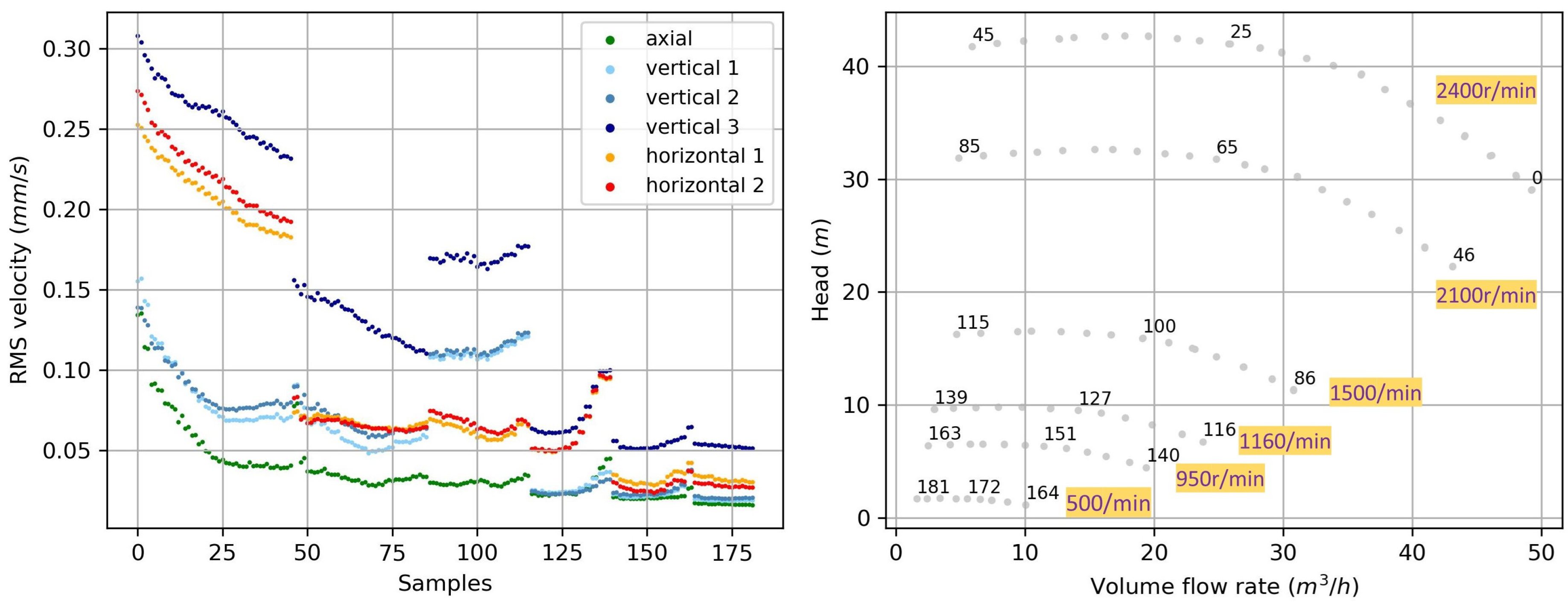
The acceleration is converted into velocity using numerical integration [15]. After implementing a highpass filter with a cutoff frequency of 5 Hz, the acceleration is cumulatively integrated using the composite trapezoidal rule. The Root Mean Square (RMS) velocity of each operating points is calculated, Figure 6 (left). For clarity, part of the sample numbers and rotational speeds are marked in the overview diagram (e.g., sample 0: top right point with 2400 r/min). The maximal RMS velocity of six sensors are listed in

Table 1. Maximal RMS velocity and velocity range limits in ISO 10816.

Max. RMS Velocity (mm/s)			Velocity Range Limits for Class I (mm/s)
axial	vertical 1/2/3	horizontal 1/2	good: <0.71 satisfactory: <1.80
0.14	0.16/0.14/0.31	0.25/0.27	unsatisfactory: <4.50 unacceptable: >4.50

. In comparison with the velocity range limits of standard ISO 10816, it is concluded that the pump works in good condition. Besides, a comparison between the measured operating points and the characteristic curves (Q-H curve) in the manual is performed. A good agreement further ensures that the pump works in normal status and that the measuring devices in the test rig is working properly.

3.2. Experimental Setup

The experiments are conducted on GeForce GTX 1080 Ti with CUDA version 11.4. The Adam optimizer with a learning rate of $5\times {10}^{-4}$ and weight decay of $8\times {10}^{-4}$ is used [16]. The adopted loss function is MSE loss, which measures the mean square error (squared L2 norm) between prediction $\widehat{y}$ and target y. It is described as:

$$l(x,y)=mean\left({\{l_1,...,l_i,...,l_N\}}^T\right),l_i={(y_i-\widehat{y_i})}^2,$$

(4)

where N is the batch size.

3.3. Baseline Experiments

For the baseline experiment, a single signal or a combination of three signals is fed into the network, and no data augmentation methods are implemented. For each input signal, the training process is repeated 20 times, and the final estimation of the operating point is calculated as the mean value over all repetitions. The dataset consists of 182 samples measured under different rotational speeds, and it is randomly split into train set (70%), validation set (15%) and test set (15%). The validation set is used to choose the model with the lowest loss during the training process, which avoids overfitting to a certain extent. To ensure a fair comparison, the split of dataset remains the same in all experiments using a specified random seed.

Table 2. Result of baseline experiment.

	Signals	MSE Loss	Mean Relative Error of Flow Rate/Head (%)
1	axial accelerometer	3.53	10.19/2.81
2	vertical accelerometer 1	3.45	11.61/3.68
3	vertical accelerometer 2	2.94	9.79/3.04
4	vertical accelerometer 3	1.69	7.23/2.37
5	horizontal accelerometer 1	3.38	9.33/3.49
6	horizontal accelerometer 2	3.00	9.53/2.17
7	microphone 1	2.48	10.29/3.22
8	microphone 2	2.43	10.47/3.87
9	1&4&6	2.42	7.55/1.81
10	4&6&8	1.76	7.46/2.26
11	4&7&8	1.83	7.32/3.09

shows the result of the baseline experiments. Besides the MSE loss, the mean relative error of the estimation for flow rate and head are also listed. Notice that some operating points lie near the zero point. For these points, although the absolute error is small, the relative error is large. To avoid affecting the representativeness of the results, those points ($h<0.1h_{max}$ or $Q<0.1Q_{max}$) are not counted in the statistics. The mean relative error is calculated as follows:

$$e_r=\frac{1}{N_T}\sum _{i=1}^{N_T}\left|\frac{y_i-\widehat{y_i}}{y_i}\right|,\widehat{y_i}=mean\left({\left\{\widehat{y_{i,1}},...,\widehat{y_{i,20}}\right\}}^T\right),$$

(5)

where $N_T$ is the number of samples in the test set after removing small values, $y_i$ is the target and $\widehat{y_i}$ is the mean of 20 estimations.

The signal “vertical accelerometer 3” located on the base of the pump unit shows the smallest MSE loss—almost half of the axial accelerometer. The mean relative error of “vertical accelerometer 3” also outperforms other input signals: 7.23% for flow rate and 2.37% for head. The signal collected from the base includes more useful information for the estimation of operating points. For all input signals, the mean relative error of head (around 3%) is always smaller than that of flow rate (around 10%).

The signal from the base is vulnerable to fixing methods and other pump units in the laboratory that may exist in the further research. An over-reliance on such signals may not provide a generalized and robust model. Hence, in addition to experiments with a single signal, three combinations are also tested to explore if the fusion of data from different sensors brings extra improvement of performance. The combination 1, 4 and 6 consists of signals from accelerometers in three directions, each of that showing the best results in single signal experiments. The combination 4, 6 and 8 includes signals from two accelerometers and microphone 2. The combination 4, 7 and 8 consists of signals from microphones on both sides and the accelerometer on the base.

During preprocessing, instead of repeating the first dimension of a single signal three times, three different signals are stacked to build the input matrix with shape (3, 224, 224). For experiment 9 and 10, although the MSE loss is not smaller than experiment 4, the mean relative error represents a similarly good performance as experiment 4. In total, the combination of single signals brings no significant improvement on the current result, but considering the susceptibility of single signal, two combinations (No. 9 and 10) provide a stable alternative of “vertical accelerometer 3” for future applications.

3.4. Data Augmentation

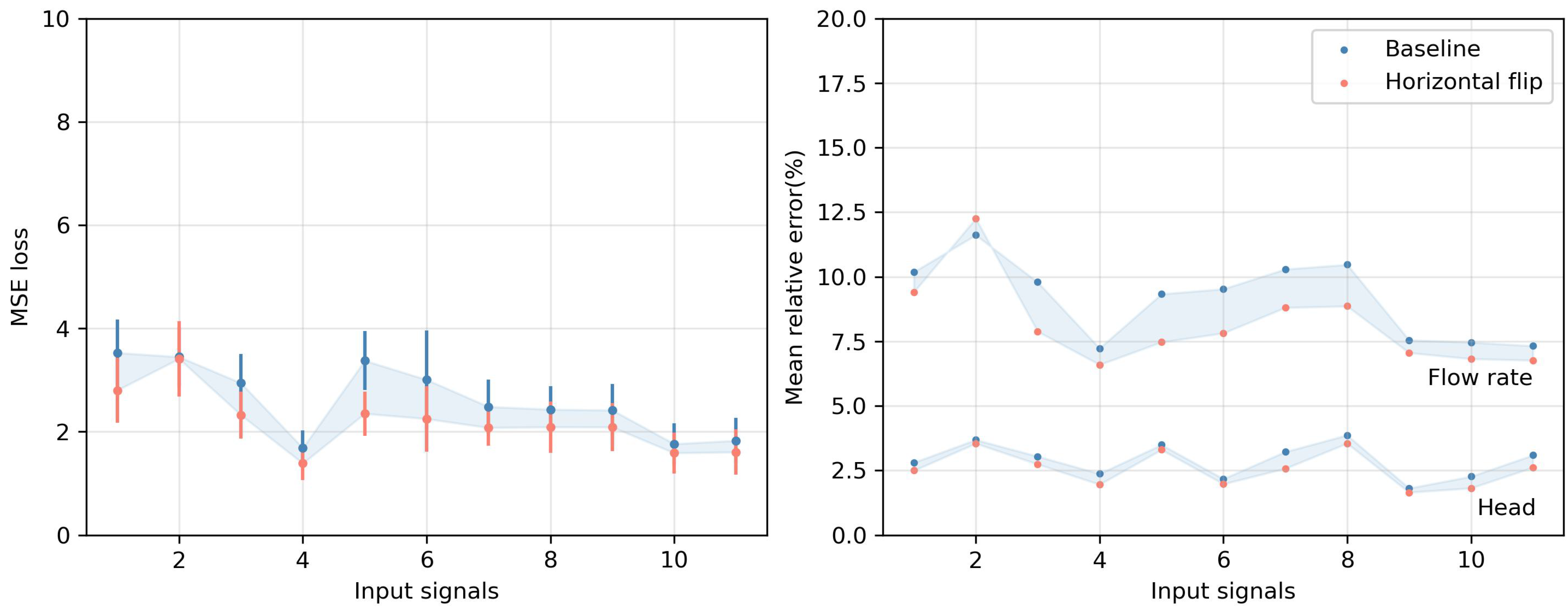
In applying the horizontal flip as an augmentation method, the comparison with the baseline experiment shows that the losses for all input signals are reduced, Figure 7. The left part shows the mean and the standard deviation of MSE loss among 20 repetitions. For input signal “vertical accelerometer 1” (No. 2), the decline of MSE loss is insignificant. The mean relative error of the flow rate dropped for almost all input signals.

It is observed that for input signal “vertical accelerometer 1”, the relative error of the flow rate rises from 11.6% to 12.3% after horizontal flip. It occurs because the reduction of loss, which is a metric of absolute distance between prediction and true value, does not always guarantee the reduction of the relative error. However, training of the network using a loss measuring relative distance provides no improvement. The possible reason is that the relative loss function makes the train process harder. The mean relative error for head in the baseline experiment is already very small—it decreases slightly.

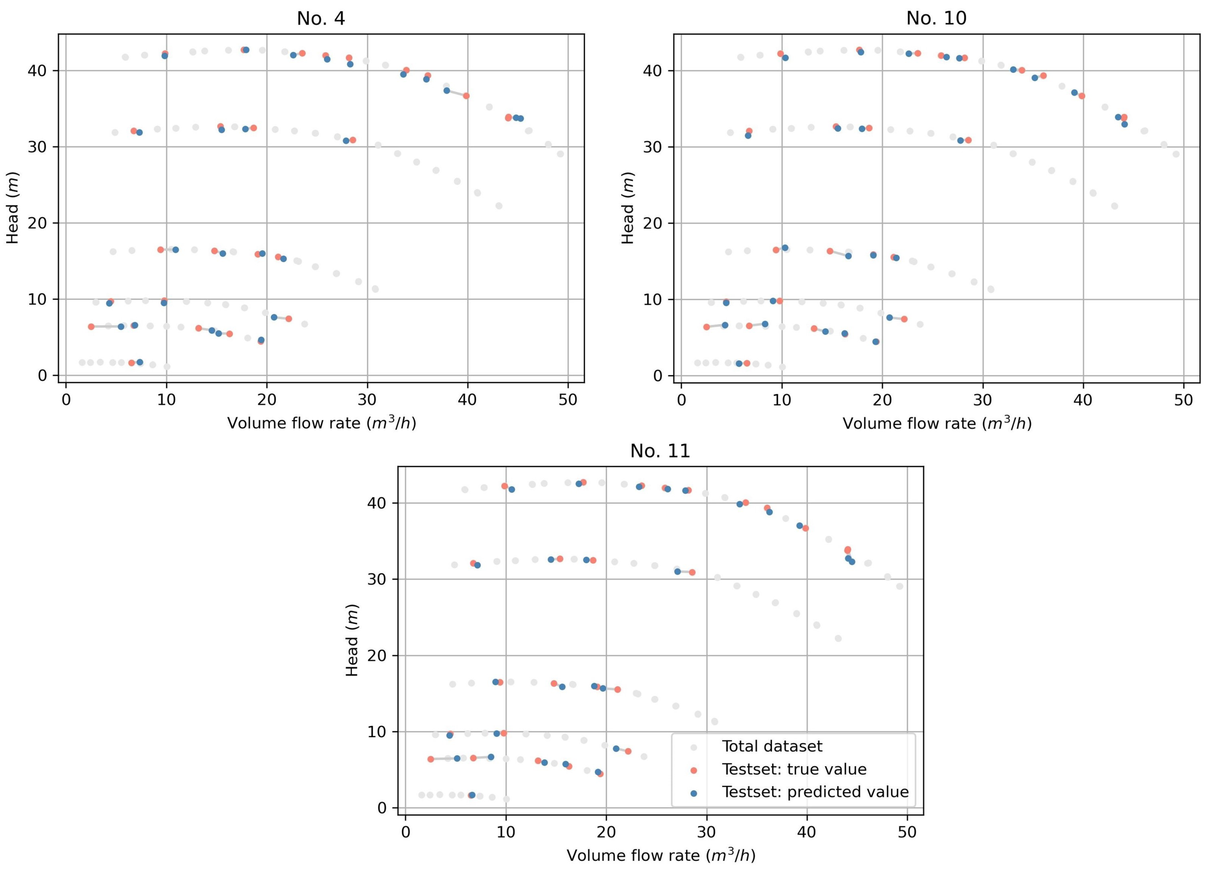
The result of applying a sliding window is presented in Figure 8. The size of the dataset is expanded with factor 3. For all single signals and signal combinations, the MSE losses and relative errors are significantly reduced. The standard deviation is smaller than baseline experiments. This augmentation method works pretty well in our application. The three best results are from experiments 4, 10 and 11, reaching a mean relative error of 3.55%/1.35%, 4.20%/1.36% and 4.37%/1.70% for flow rate and head, respectively. The predicted operating point (red) and true value (blue) of these best models are shown in Figure 9. For clarity, the operating points in the total dataset at six rotational speeds are plotted. The grey line between red and blue points indicates the distance of the true operating points and corresponding prediction.

4. Conclusions

Vibration and acoustic signals are collected from a test rig. A suitable preprocessing method for the raw time signal is chosen. The plausibility of the method is analyzed based on the vibration velocity limit listed in ISO 10816. For baseline experiments, the modified ResNet18 is trained using input signals from single sensors or a combination of different sensors with 20 repetitions. The estimation result of the vertical accelerometer located on the base outperforms other sensors, the MSE loss equals 1.69 and the mean relative error is 7.23% for flow rate and 2.37% for head. The result of the other two signal combinations also represents similar performance. Considering that a single signal from the base can easily be affected by the fixing method and the environment, the combination of signals probably has more potential for further research.

Applying a sliding window and horizontal flip as a data augmentation method, the result of estimation is further improved for all input signals. A sliding window with factor 3 shows significant reduction in MSE loss and relative error. The three best results from experiments 4, 10 and 11 reach a mean relative error of around 4% for flow rate and 1.5% for head. In the proposed plan for the next phase, it is intended to measure a bigger dataset with a longer time series. In doing so, a comparative analysis between the data augmentation and the bigger dataset will be carried out.

The proposed method indicates that the estimation of the operating point of the pump using vibration and sound with the help of CNNs is feasible within the relative error values obtained as results. The assessment whether the accuracy of the current prediction of the operation points is sufficient for predictive maintenance will require additional work. The current results were obtained in an anechoic chamber. Additionally, there is no defect on the machine and other elements connected to it. But in real life, degradation of machinery (blade erosion due to abrasive particles) and improper or delayed maintenance exist. These will lead to the change of characteristics, even if only in a limited way. Achieving a more robust estimation model for real-life applications still requires a lot of subsequent research.

For further research, the pump unit will be moved out of the anechoic room, and the influence of the noise from other facilities in the laboratory will be investigated. Besides, more sensors will be implemented such as structure-borne sensors. To obtain a more general model that performs well for different pumps, e.g., the same type with the same size, same type with different size, and even different types, it is valuable to collect various data and explore the transferability between pumps. In addition, the methodology that has been presented for the estimation of the operating point possesses the potential to be extended for the purpose of condition monitoring and fault diagnosis using acceleration and noise.