Article

Experimental and Numerical Analysis of a Compressor Stage under Flow Distortion

1
Univ. Lille, CNRS, ONERA, Arts et Métiers Institute of Technology, Centrale Lille, UMR 9014-LMFL-Laboratoire de Mécanique des Fluides de Lille -Kampé de Fériet, F-59000 Lille, France
2
Onera—The French Aerospace Lab. F-92190 Meudon, France
*
Author to whom correspondence should be addressed.
Int. J. Turbomach. Propuls. Power 2021, 6(4), 43; https://doi.org/10.3390/ijtpp6040043
Submission received: 30 September 2021 / Revised: 2 October 2021 / Accepted: 17 November 2021 / Published: 23 November 2021

Abstract

:
On many occasions, fan or compressor stages have to face azimuthal flow distortion at inlet, which affects their performance and stability. These flow distortions can be caused by external events or by some particular geometrical features. The aim of this work is to propose a joined numerical and experimental analysis of the flow behavior in a single axial compressor stage under flow distortion. The distortions are generated by different grids that are placed upstream to the rotor. Experimentally, the flow analysis is based on the measurements obtained by a series of unsteady pressure sensors flush-mounted at the casing of the machine rotor. URANS computations are conducted using the elsA software. The flow distortion is simulated by a drop of stagnation pressure ratio at the inlet boundary condition. The study is focusing first on the ability of a pressure drop, imposed as an inlet boundary condition in CFD, to reproduce accurately the effect of a flow distortion. The analysis is conducted using singular value decomposition (SVD) and dynamic mode decomposition (DMD). A special attention is then paid, on the experimental level, to the arising of rotating stall, from the onset of the instability up to completely developed stall cells.

1. Introduction

Inlet distortion is the situation in which the flow entering turbomachinery is nonuniform. This can occur in jet engines because the curvature of the intake induces secondary flows, or because the intake is close to the fuselage, so that the boundary layer is ingested. In principle, the boundary layer ingestion (BLI) has a potential benefit on fuel consumption for civil aircrafts [1]. It consists of reducing the drag using the aircraft engines, which are partially embedded at the back of the fuselage of the aircraft and ingest the boundary layer developed on the fuselage. Other situations in which distortion can occur relate to the operation of the engine in highly turbulent or in crosswind flows. A typical feature of a distorted flow is the co-existence of regions of lower and higher total pressure. Indeed, turbomachines are normally designed to work under a circumferentially uniform inflow, so that the rotating blades see the same angle of incidence and experience equal blade pressure profiles. However, in a circumferential distorted flow, the blades rotate in and out of the low pressure region and thus they will experience a cyclically varying incidence.
A simple model to describe the circumferential distortion was given by [2]. The response of the blades to a sinusoidal oscillation of the incidence angle consists of an oscillation of lift coefficient and, since the variations in pressure ratio are proportional to the variations in lift coefficient, the cyclic behavior of the lift coefficient induces a cyclic behavior of the pressure ratio in the compressor map. This cyclic behavior causes a degradation of the performances of the machine, which cannot sustain the same pressure ratio as in nondistorted operational regimes. Moreover, as far as the compressor stability is concerned, the distorted flow region causes a higher incidence, and thus operation closer to the stall limit. Stall margin is reduced and instabilities will be triggered for a higher flow coefficient.
From the early studies in the 1970s [3,4] up to more recent studies [5], the effect of inlet distortion on turbomachines has been tested mostly by means of screens [6] placed in front of the machine; the attention has been concentrated on the characterization of the steady state performance under inlet distortion, and on rotating stall mostly in terms of stall margin reduction. Two aspects appear to deserve further investigation.
The first relates to the characterization of the effect of screens to represent a distortion. A better understanding of the effect of the geometry of the screen on the flow is needed to improve the understanding of the effects of screen-generated inlet flow distortion. A second aspect is the lack of investigation of the detailed dynamics of stall inception under distortion [7].
To address the first topic, experimental and numerical signals in steady state and transient operation of an axial flow compressor were compared, both in the case of clean undistorted flow operation and distorted flow operation created by a screen placed in front of the machine. Experimental and numerical casing pressure signals were compared for a stable operating point close to nominal conditions. As far as the stable operation is concerned, instantaneous casing pressure measurements were analyzed using dynamic mode decomposition to extract the modal content of the signal and to highlight the effect of the screen.
As far as the detailed dynamics of the transient operation towards rotating stall are concerned, casing static pressure has been acquired with sensors distributed circumferentially and used to track the evolution of the perturbation during transient.

2. Experimental Setup

The experiments were performed on the low speed CME2 axial compressor operating at Arts et Métiers, Lille, France. Its main operating and geometrical parameters are listed in Table 1.
The test bench (Figure 1b,c) is equipped with 14 casing flash-mounted pressure sensors (Figure 2). Seven piezoresistive pressure transducers ENDEVCO 8510B are placed circumferentially at mid chord, while seven other piezoresistive pressure transducers ENDEVCO 8507C are mounted onto an instrumented window (Figure 1c) and form a line in the axial direction starting from 2 mm ahead of the leading edge of the blades and continuing up to the trailing edge. The 0° position is chosen at noon in Figure 1b, and positive angles are in the blades’ rotation direction. The sampling rate is 100 kS/s. The rated pressure of the transducers is 6.89 kPa, and the sensitivity after calibration varies between 23.1 and 29.8 mV/kPa. The error in % of the full scale is between 0.3 and 1.2.
The distortion is generated through distortion screens created from steel perforated plates installed one hydraulic diameter in front of the compressor. The plates are 2 mm thick with 3 mm diameter holes (d in Figure 1a) and 5 mm inter-hole distance (h in Figure 1a) and an equilateral triangle pattern (Figure 1a). The porosity, defined as perforated area divided by total area is f = π 2 3 ( d h ) 2 = 33 % . The plates were cut into angular sectors to mimic a circumferential distortion (Figure 1b). For the experiments, a sector of 60° has been installed between 270° and 330°; the estimated nondimensional pressure drop based on the velocity where the screen is placed (22 m/s) is 1.05.

3. Numerical Setup

Unsteady RANS computations are performed on this configuration with the ONERA compressible solver elsA [8] using a second-order in space Roe scheme, a first-order in time Backward Euler scheme and a scalar LUSSOR implicit method. The turbulent quantities are determined using the k-l two-equation model of [9]. The full annulus geometry is computed with the struts, rotor and stator rows, leading to a mesh of 122 million nodes as illustrated in Figure 3. The nodes in the strut, rotor and stator meshes are respectively 10, 70, 42 million. There are 88 and 121 nodes in the spanwise direction for the strut and stator components, respectively. In the rotor tip clearance, the number of spanwise nodes is 33. The geometry of the screen is not simulated; rather, the screen-induced distortion has been modelled by a total pressure drop directly applied at the inlet boundary condition. The inlet condition consists of of applying total pressure, total temperature, velocity direction and turbulence variables (turbulent rate of 2%); the outlet boundary condition is applied with a static pressure at the hub and a radial equilibrium condition, and it has been used for both simulations with and without the grid. There were 3600 iterations per rotor revolutions used for the computations, and 6 complete revolutions were simulated for both clean and distorted cases. As far as the time periodicity of the numerical simulations is concerned, the criterion used consists of a periodic repeatability of the instantaneous mass flow for two consecutive revolutions with discrepancies of less than 0.1%. Time averaging was performed on a full rotation of the rotor.
Two simulations were performed: a first one with a clean inlet flow, a second one with a pressure drop corresponding to the first screen used in the test. The two simulations without the grid and with the 60° grid converged toward a stable operating point, without rotating stall, at an average mass flow respectively of 4.853 kg/s and 4.848 kg/s respectively. Unsteady pressure was extracted from the calculations at the same fixed positions as the piezoresistive pressure transducers of the test bench.

4. Results

4.1. Stable Operation

A comparison was performed between the signals measured ahead of the rotor for the nondistorted and 60°-screen-distortion cases. The comparison was made using the Dynamic Mode Decomposition (DMD). The DMD was first proposed by [10], and it is a data-driven method that provides a way to decompose spatio–temporal measurements into a set of dynamic spatio–temporal modes derived from a local linearization of the system dynamics. The modes were limited to the postprocessing of the time-dependent pressure measurements as we did not combine multiple probes to include the spatial information in our DMD analysis.
The measurements of pressure in time were rearranged in a matrix H (Hankel matrix) by shifting them in time according to the number of modes we employed for reproducing each signal. Hence, the number of columns of H was equal to the number of modes that were used to approximate the signal (500 in the study); the number of rows corresponded to the number of time measurements considered in the postprocessed time window (5 s × 100 kS/s).
From the H matrix, two matrices X1 and X2 were created, X2 being the time shifted matrix, and X1 the matrix of the individual snapshots. The DMD computed the leading eigenmodes of the linear operator A that best advanced the data X1 to X2, i.e., X2N ≈ A X1N−1, where N denotes the time of the current snapshot. For N→∞, hence marching continuously in time, the corresponding linear system reads
d X d t = A X .
When subjected to initial condition X ( 0 ) , the equation has the solution:
x ( t ) = k = 1 N ψ k   exp ( ω k t ) b k
where ψ k and ω k are the eigenvectors and eigenvalues of the matrix A , while b k are the coordinates of x(0) in the eigenvector basis. Getting back to the analogous time-discrete system with time step Δ t , it yields
X 2 = A   X 1
with A = exp ( A   Δ t ) . Since the A matrix has generally a very large dimension, instead of computing directly the eigenvalues of A, we employed a rank-reduced representation of A. This rank-reduced representation of A was obtained using Singular Value Decomposition (SVD). The full algorithm employed in our study is explained in more details in [11].
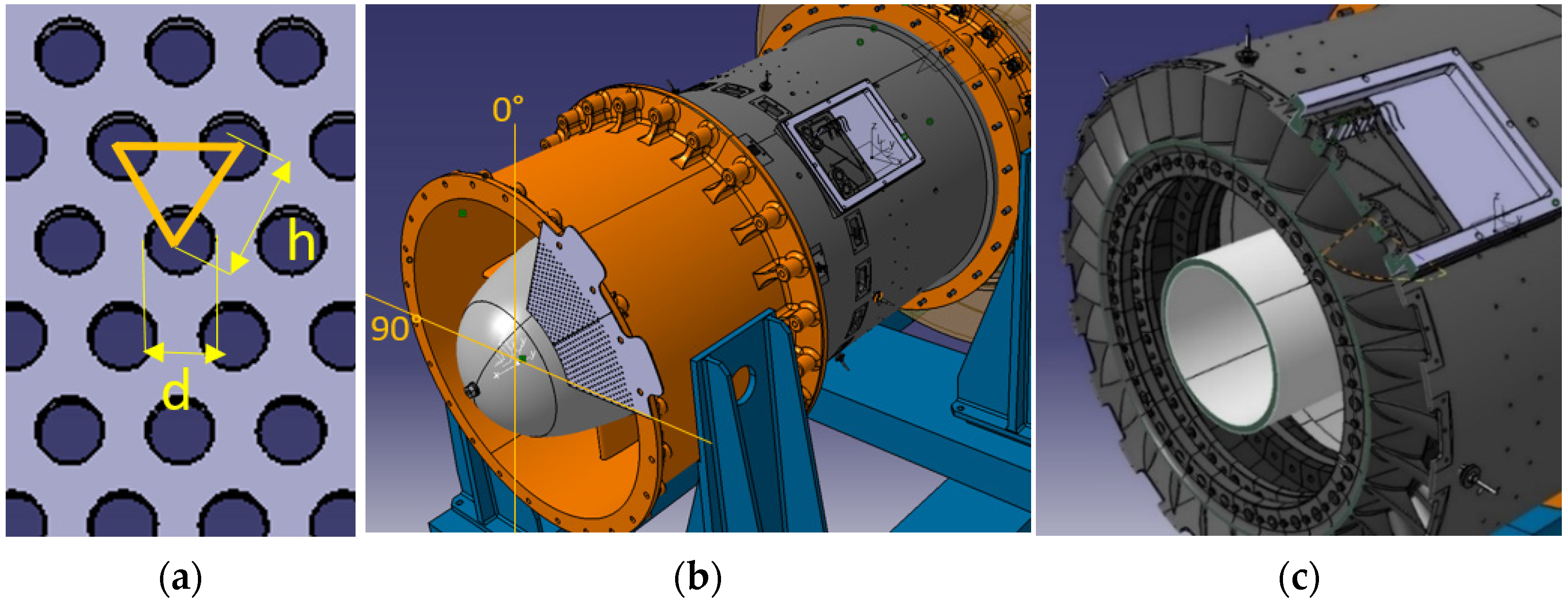
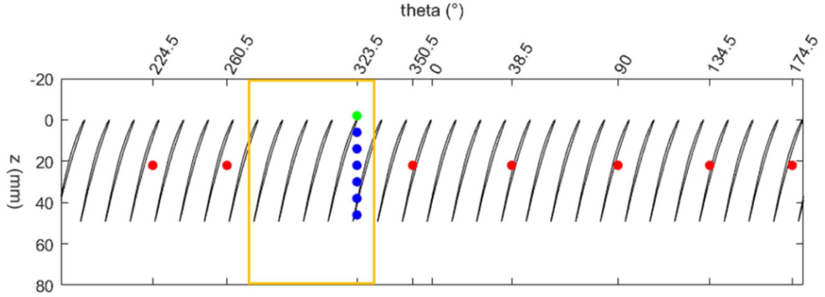
First, DMD was applied to the experimental signals. In the present experiments, two different mass flow rates were chosen and casing static pressure from the sensors placed at z = 2 mm (green in Figure 2) was recorded for 5 s, which was approximatively 265 rotor revolutions. The first mass flow rate was 5 kg/s and it corresponded to a flow coefficient ϕ of 0.506 close to design point.
The second mass flow rate we investigated was 4.2 kg/s and it corresponded to a ϕ of 0.425, i.e., the last stable configuration before the onset of rotating stall in CME2. 
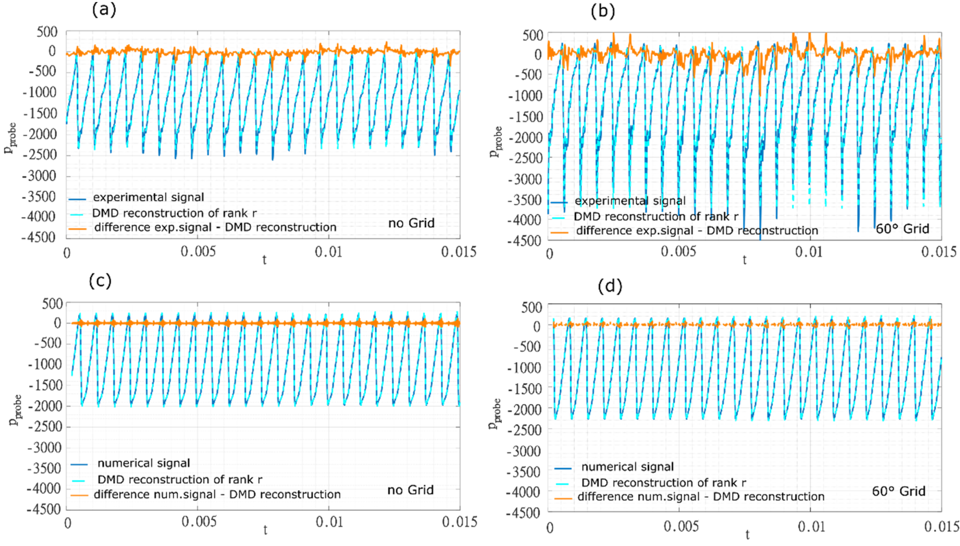
Figure 4a,b depicts the comparison between the DMD reconstruction and the raw signals experimentally obtained. On the same Figure, the error of the DMD reconstruction is plotted in orange. The DMD reconstruction is good, but it loses some accuracy when some nonperiodic peaks occur in the experimental signal at 5 kg/s, and it does not provide an accurate approximation of the grid distorted signal at a mass flow rate of 4.2 kg/s (not represented in Figure 4) because the signal was strongly nonperiodic.
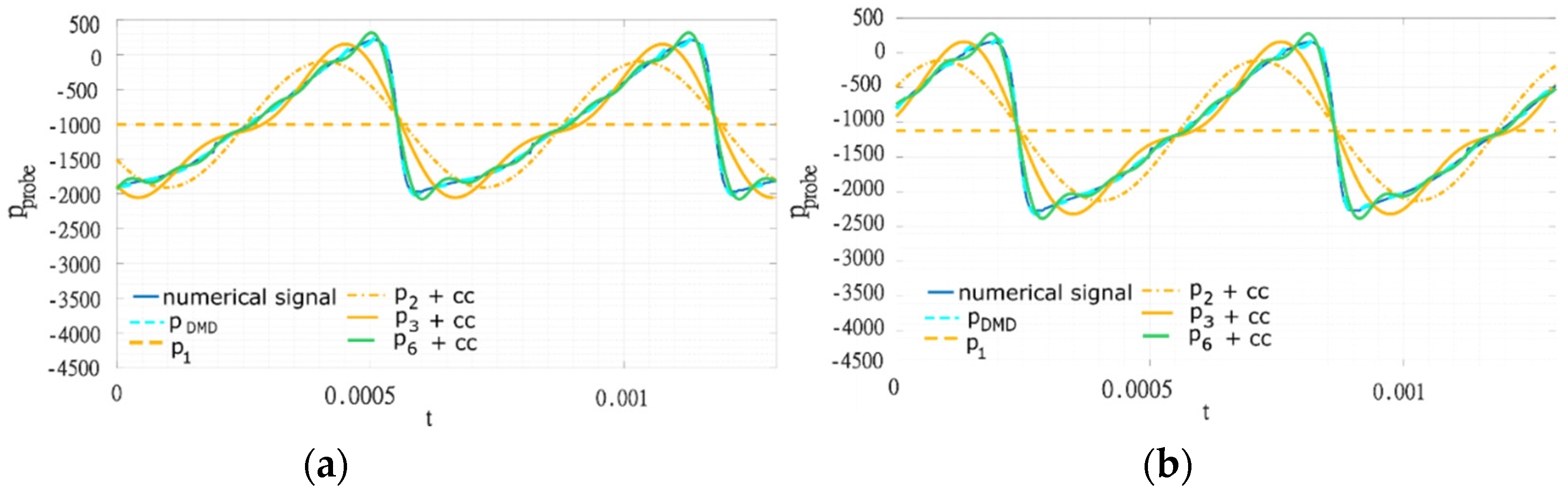
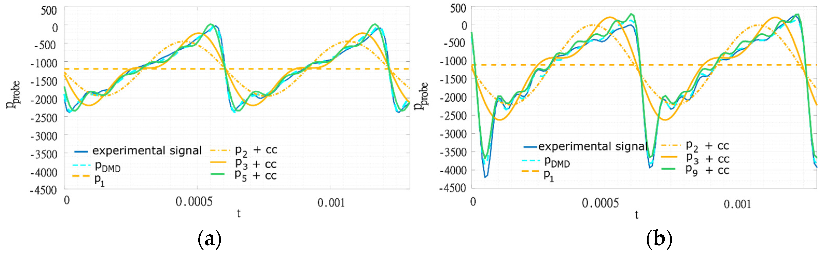
A partial DMD reconstruction is shown in Figure 5a,b, where pDMD indicates the reconstruction with 21 modes, p1 the first mode reconstruction (the linear least-squares fit of the signal), p2 the reconstruction up to the second order (linear least-squares fit plus the second mode with its complex conjugate), and so on. In Figure 5a,b, p5 and p9 respectively represent the DMD reconstruction with the minimum number of modes that have an error less or equal to 5% with respect to the DMD with 21 modes.
According to this criterion, the minimum number of DMD modes required to well reproduce the experimental signal was 11 for the nondistorted case at a mass flow rate of 5 kg/s. The required minimum number of modes grew to 19 when the grid was introduced. These additional modes can be partly explained by the presence of a low pressure peak in the signal, a trace of increased blade loading due to the locally reduced mass flow rate behind the grid. But we anticipate that this is not the only effect of the presence of the grid.
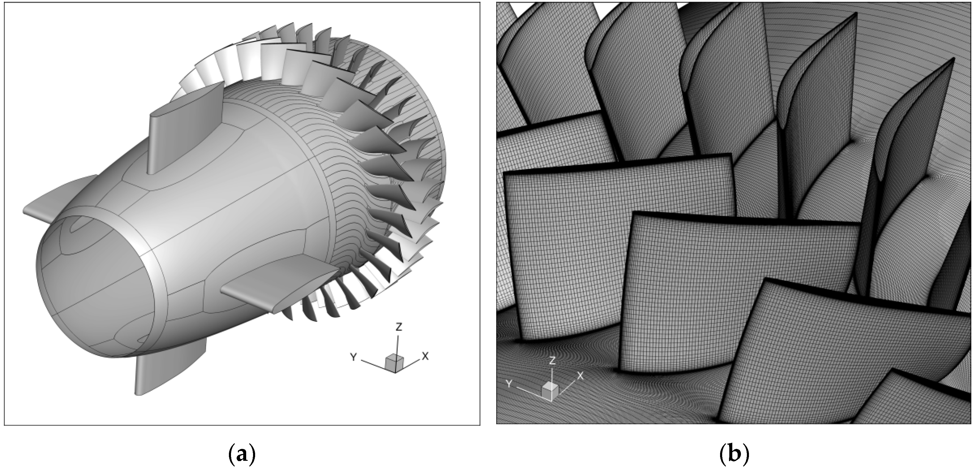
The DMD was then applied to numerical signals. The reconstruction (Figure 4c,d) was very good. For the numerical signals, the required number of DMD modes to well reproduce the signal was 13 no matter the presence of the grid (Figure 6a,b). Numerical simulations are thus losing some information compared to experiments.
The first qualitative difference between the experimental and numerical signals was the presence of a sharp pressure drop in the experimental signal. Such a feature was not captured by the numerical simulation. A second difference was the presence of high-frequency oscillations in the experimental signal (Figure 5b). Modes with 5 and 10 oscillations per blade channel emerged. Their amplitudes were respectively the 25% and 7.5% of the amplitude of the main harmonic. Such modes can be related to the jets created by the holes of the grid. The blade channel measures 57 mm and the distance between the holes is 5 mm so that there are 11 holes per blade channel. This feature already highlights the limitation of using a grid to reproduce a generic distortion since the grid geometry introduces in the flow some characteristic scales that are not existing in other types of distortion. Consistently, the comparison between Figure 5 and Figure 6 shows that an inlet total pressure drop is too simplistic for modeling a screen-generated distortion.
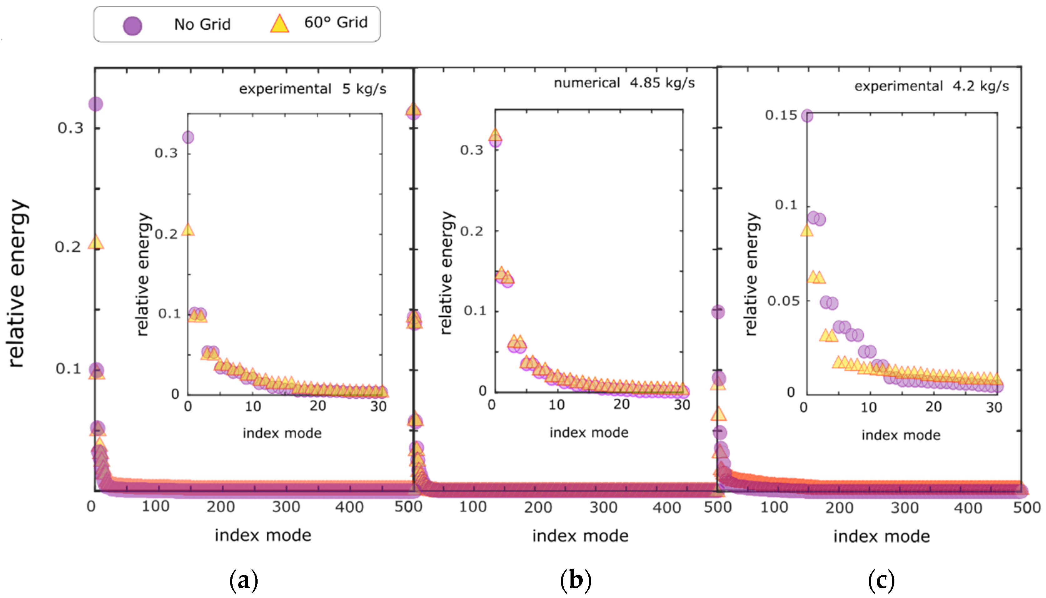
In Figure 7, the eigenvalues obtained from applying SVD to the experimental signals are represented for the two mass flow rates investigated experimentally, with and without the presence of the 60° grid. The SVD eigenvalues are also represented for the numerical signals with and without the grid. The eigenvalues are normalized on the value of their total sum such that they represent the relative energy content of the various SVD modes. In the numerical signals (Figure 7b), the presence of the grid did not change the relative energy content of the modes. Moreover, in the experimental signals (Figure 7a,c) there were significant differences. We stress that the distribution of energy was different depending on the mass flow rate, even for nondistorted experimental flow. The first mode of the SVD (violet in Figure 7) had a relative energy of 32% at 5 kg/s, that decreased to 15% at 4.2 kg/s.
Thus, as the stall limit is approached, signals were less periodic and the energy was redistributed from low frequencies to higher frequencies corresponding to higher index eigenvalues. The presence of the 60° screen had a similar effect on the redistribution of the energy of the SVD modes, i.e., part of the low-modes energy of the configuration without the grid was transferred to higher modes for the system with the grid. In fact, with the grid (orange in Figure 7), the relative energy of low index modes was lower than without the grid (violet in Figure 7), while the relative energy of high index modes with the grid was higher than without the grid.
The tendency was reproduced for both 5 kg/s and 4.2 kg/s. We speculate that a part of the energy redistribution was caused by the additional presence of the modes introduced by the local geometry of the grid.

4.2. Stall Inception

As shown in the previous section, the numerical simulations well captured the leading-order effect measured in the experimental signals for distorted configurations. We anticipate, however, that the grid-geometry-induced features observed in the experimental pressure measurements play a major role in the onset and decay of rotating instabilities. Since the numerical perturbation was modeled as a pressure drop, such a physical phenomenon cannot be studied with our computational simulations. Hence, in the following, only experimental measurements are presented.
As far as the stall inception process is concerned, the case without distortion screen and the case with the 60° distortion screen upstream of the instrumented window were compared. The throttling valve was closed progressively, starting from the last stable point to induce rotating stall. It has been observed, in previous works [12,
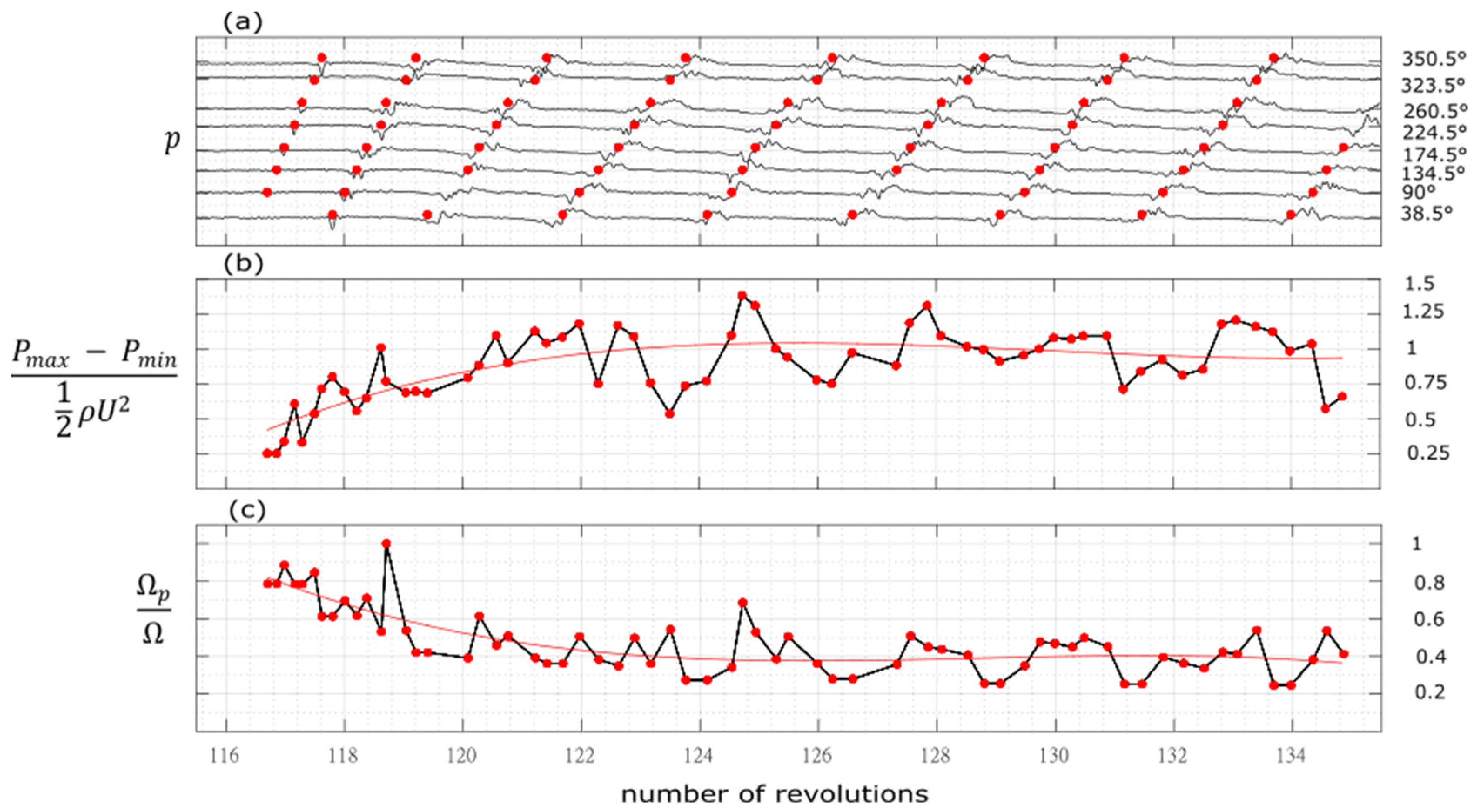
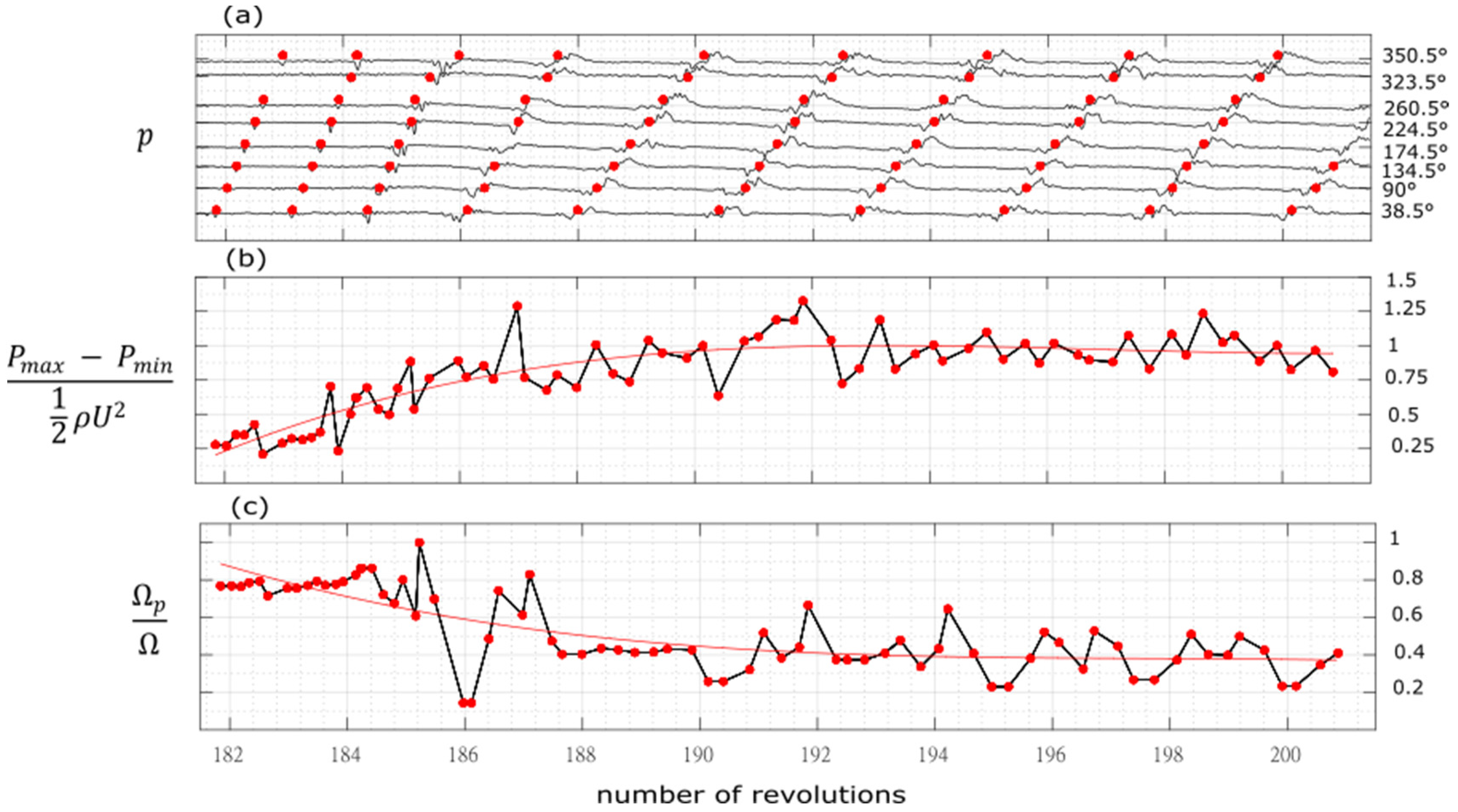
13] that the perturbation arising in CME2 is always of spike type. A typical transition to stall is represented in Figure 8. The signals were filtered (cut frequency 800 Hz) to eliminate the blade passing frequency (1600 Hz). The tracking of the perturbation development was done by using cross correlation between each signal and a reference piece-wise signal composed of a typical spike, a stall cell and a transition between the two. The peaks of the correlation represent the time position of the perturbation for each sensors (red dots in Figure 8).
They were then used to derive the perturbation speed (Figure 8c). The peak-to-peak amplitude of the perturbation is also reported (Figure 8b). The main differences concern the starting point of the perturbation and the development of the perturbation during the first revolutions. The first difference is the stalling mass flow rate observed experimentally: 4.15 kg/s without grid and 4.23 kg/s with the 60° grid.
In the undistorted case, the spike usually starts in the region between 90° and 135°.
Such a feature has a very high reproducibility, most likely because the tip clearance in that region decreases and reaches the minimum value due to the imperfect circularity of the casing as already observed [13]. The perturbation then develops rapidly (in about 5 rotor revolutions) in amplitude, while its speed decreases from about 90% to 40% of the rotor speed.
In the distorted case, however (Figure 9), the perturbation arises just after the grid (around 30°). The explanation can be attributed to the fact that the region of highest incidence was located at the exit of the distorted region (in the direction of rotation) [14]. This is due to the pressure gradients created by the interaction of the low-pressure distorted stream and the undistorted one: these gradients created an upstream flow redistribution, so that the incidence at the entrance of the distorted region was reduced and the incidence at the exit was increased. In 
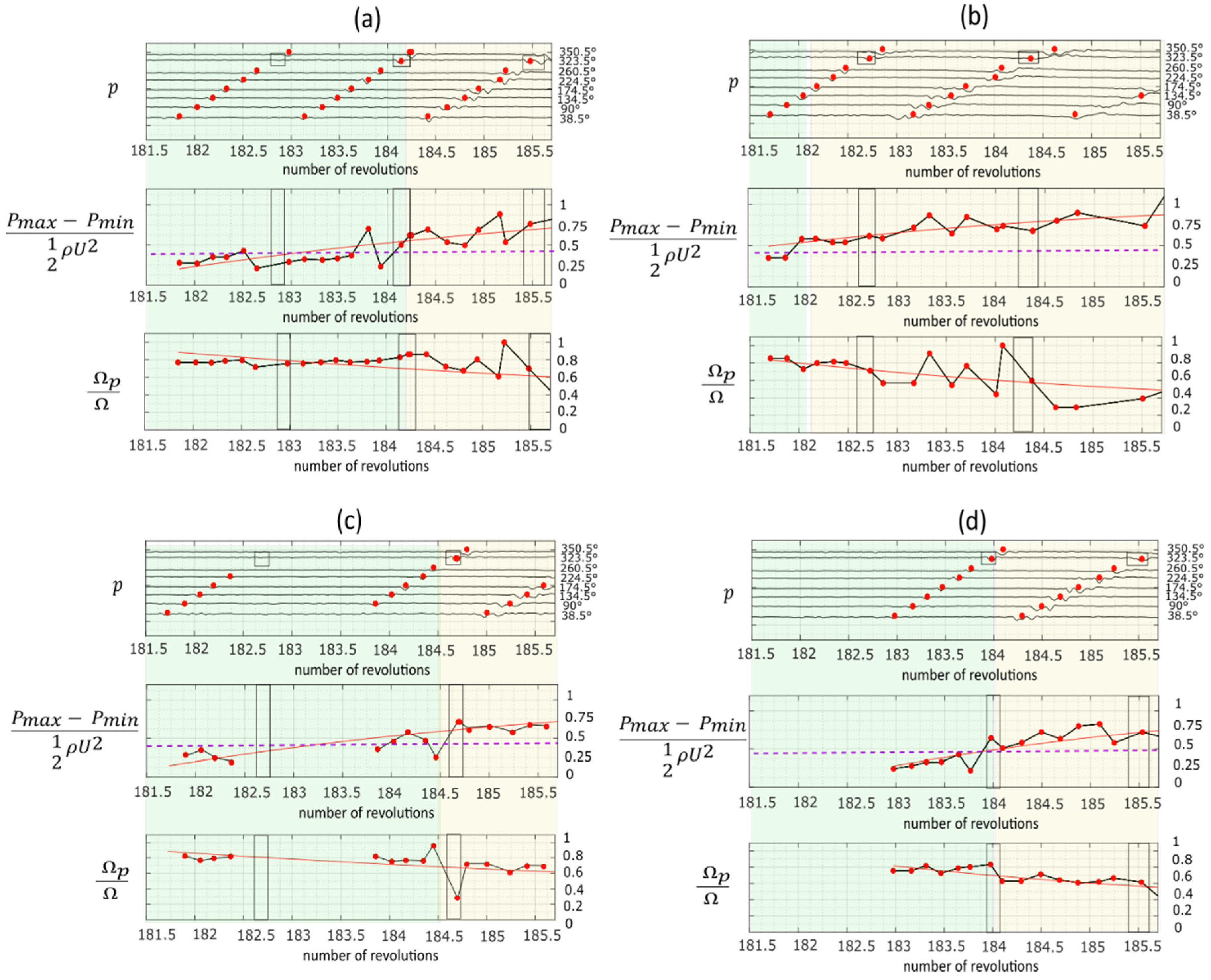
Figure 10, four repetitions of stall transient with the 60° grid are reported. The four transients were obtained throttling the compressor at a constant throttle speed, starting from the same mass flow rate corresponding to the last stable point of its characteristic curve. In the two cases in Figure 10a,c, after a period of growth, the perturbation vanished just before entering in the distorted region (represented with a black rectangle), which is exactly in the region of reduced incidence argument just discussed. The disappearance of the spike, however, was not always reproducible. It can occur multiple times before rotating stall, or it can also never occur (two cases in Figure 10b,d). The results reported in Figure 10 suggest that a threshold value in the perturbation amplitude at the beginning of the distorted region exists, above which the perturbation continues to grow. This threshold value is about 0.425 of the dynamic pressure based on the blade tip speed. There is thus a clear competition between the stabilizing effects of the low-incidence region existing at the distortion inlet and the proper dynamic of the instability.
Moreover, this threshold value also marks two different stages of the development of instability (Figure 10): a first stage characterized by amplitudes lower than the threshold and constant rotational speed of the perturbation, and a second stage characterized by amplitudes higher than the threshold and decreasing speed of the perturbation.
This reflects the fact that when the perturbation started, nonlinear effects were weak, and were responsible for the saturation that limited the intensification of the perturbation, but the process of intensification of the perturbation did not affect the speed of the perturbation. Instead, as soon as the perturbation reached a high enough amplitude, nonlinear effects became significant and led to a saturation of the intensification process, as well as to a remarkable slowdown of the convective velocity due to the enhanced inertia of the established perturbation.
Apart from the initial stages of the perturbation, the experiments showed that the development into rotating stall is very similar, independently of the presence of the grid. The developed rotating stall cell has a speed corresponding to 40% of the rotational speed of the rotor, while its pressure amplitude is equal to the dynamic pressure based on the blade speed.

5. Conclusions

Unsteady casing pressure measurements were performed on an axial flow compressor, under clean flow and circumferential distorted flow, at two mass flow rates in the stable part of the compressor characteristics and at a varying mass flow rate, obtained throttling the valve from the last stable point to induce rotating stall. The analysis through DMD showed that the effect of the grid was to introduce new modes in the signal (both in the case of a real perforated plate and in the case of a simulated uniform low total pressure region). The modes introduced in the experimental signal have multiple oscillations per blade channel, reasonably due to the geometry of the holes of the grid, which are not simulated in the numerical case. Moreover, the grid induces a redistribution of energy from low frequency modes to higher frequency modes.
Some variability in time of the onset of the spike perturbation was found, even if a correlation was confirmed between the spike occurrence and the location of the grid. Moreover, the spike dynamics seems to be determined by a critical pressure amplitude criterion.

Author Contributions

A.B.: experimental work, formal analysis, writing manuscript; B.G.: numerical work; P.J.: validation; O.R.: validation; F.R.: formal analysis, validation; R.B.: numerical work, validation, project administration, funding; A.D.: validation, supervision, project administration, funding. All authors have read and agreed to the published version of the manuscript.

Funding

The APC was founded by Euroturbo.

Institutional Review Board Statement

Not applicable.

Informed Consent Statement

Not applicable.

Data Availability Statement

The data will be available provided the consent of all the authors.

Acknowledgments

The work is supported by DGAC (the French Agency for Civil Aviation) through the SUBLIME research program.

Conflicts of Interest

The authors declare no conflict of interest.

Nomenclature

Roman t Time [s]
bInitial amplitude of DMD modes U = Ω r Blade velocity [m/s]
d hole diameter of the grid [m] v Axial velocity [m/s]
DMDDynamic Mode Decomposition
f Porosity of the grid [-]Greek
h grid inter-hole distance [m]σReal part of ω
p Static pressure [Pa] ϕ = v / U Flow coefficient [-]
pDMDDMD reconstructionψEigenvectors of DMD
r Compressor mean radius [m]ωGrowth rate of DMD modes
s Diagonal matrix of the SVD Ω Compressor Angular velocity [rad/s]
SVDSingular Value Decomposition Ω p Perturbation angular velocity [rad/s]

References

  1. Plas, A.P.; Sargeant, M.A.; Madani, V.; Crichton, D.; Greitzer, E.M.; Hynes, T.P.; Hall, C.A. Performance of a Boundary Layer Ingesting (BLI) Propulsion System. In Proceedings of the 45th AIAA Aerospace Sciences Meetings and Exhibit, Reno, NV, USA, 8–11 January 2007; p. 450. [Google Scholar]
  2. Melick, H.C. Analysis of Inlet Flow Distortion and Turbulence Effects on Compressor Stability; NASA Technical Report No. 2-57110/3R-3071; NASA: Washington, DC, USA, 1973.
  3. Reid, A.P. The Response of Axial Flow Compressors to Intake Flow Distortion; American Society of Mechanical Engineers: Newyork, NY, USA, 1969; Volume 79832. [Google Scholar] [CrossRef] [Green Version]
  4. Calogeras, J.E.; Mehalic, C.M.; Burstadt, P.L. Experimental Investigation of the Effect of Screen-Induced Total Pressure Distortion on Turbojet Stall Margin; NASA TM X-2239; NASA: Washington, DC, USA, 1971.
  5. Gunn, E.J.; Tooze, S.E.; Colin, Y. An experimental study of loss sources in a fan operating with continuous inlet stagnation pressure distortion. J. Turbomach. 2013, 135, 051002. [Google Scholar] [CrossRef]
  6. Davis, M.; Hale, A.; Beale, D. An argument for enhancement of the current inlet distortion ground test practice for aircraft gas turbine engines. J. Turbomach. 2002, 124, 235–241. [Google Scholar] [CrossRef]
  7. Perovic, D.; Hall, C.A.; Gunn, E.J. Stall Inception in a Boundary Layer Ingesting Fan. In Proceedings of the ASME Turbo Expo 2015, Montréal, QC, Canada, 15–19 June 2015. [Google Scholar] [CrossRef]
  8. Cambier, L.; Heib, S.; Plot, S. The Onera elsA CFD software: Input from research and feedback from industry. Mech. Ind. 2013, 14, 159–174. [Google Scholar] [CrossRef] [Green Version]
  9. Smith, B.R. A near wall model for the k-l two equation turbulence model. In Proceedings of the 25th Fluid Dynamics Conference, Colorado Springs, CO, USA, 20–23 June 1994; p. 2386. [Google Scholar] [CrossRef]
  10. Schmid, P.J. Dynamic mode decomposition of numerical and experimental data. J. Fluid Mech. 2010, 656, 5–28. [Google Scholar] [CrossRef] [Green Version]
  11. Kutz, J.N.; Brunton, S.L.; Brunton, B.W.; Proctor, J.L. Dynamic Mode Decomposition; Society for Industrial and Applied Mathematics: Philadelphia, PA, USA, 2016. [Google Scholar]
  12. Veglió, M.; Dazin, A.; Bois, G.; Roussette, O. Unsteady Pressure Measurements of Spike Type Inception in Axial Compressor: Time Frequency Analysis and Averaging Procedure. In Proceedings of the 11th European Conference of Turbomachinery, Madrid, Spain, 23–27 March 2015. [Google Scholar]
  13. Margalida, G.; Joseph, P.; Roussette, O.; Dazin, A. Comparison and sensibility analysis of warning parameters for rotating stall detection in an axial compressor. Int. J. Turbomach. Propuls. Power. 2020, 5, 16. [Google Scholar] [CrossRef]
  14. Lesser, A.; Niehius, R. Transonic Axial Compressor with Total Pressure Inlet Flow Field Distortions. In ASME Turbo Expo 2014: Turbine Technical Conference and Exposition; American Society of Mechanical Engineers Digital Collection: New York, NY, USA, 2014. [Google Scholar] [CrossRef]
Figure 1. (a) CAD representation of the equilateral triangular pattern of the grid holes; (b,c) CAD representation of the CME2 compressor showing grid position with respect to instrumented window.
Ijtpp 06 00043 g001
Figure 2. Scheme representing rotor blades and pressure probe locations highlighted in red (mid chord circumferential positions) and blue (axial position from z = −2 mm to z = 50 mm); probe used for DMD (green), wake of the grid (yellow).
Ijtpp 06 00043 g002
Figure 3. (a) CFD domain; (b) grid views.
Ijtpp 06 00043 g003
Figure 4. (a,b) Comparison between raw signal (blue) and DMD reconstruction (light blue) for the case of 5 kg/s; (c,d) comparison between raw numerical signal (blue) and DMD reconstruction (light blue) for the case of 4.85 kg/s. Difference between raw signal and DMD reconstruction plotted in orange.
Ijtpp 06 00043 g004
Figure 5. Partial DMD reconstruction; p1: least-squares fit, pi + cc: DMD modes plus complex conjugate (cc) up to i th order. (a) 11 modes 5 kg/s without grid; (b) 19 modes 5 kg/s with 60° grid.
Ijtpp 06 00043 g005
Figure 6. Partial DMD reconstruction; p1: least-squares fit, pi + cc: DMD modes plus complex conjugate (cc) up to i th order; (a) 13 modes 4.85 kg/s without grid, (b) 13 modes 4.85 kg/s with 60° grid.
Ijtpp 06 00043 g006
Figure 7. Relative energy in the modes calculated from SVD. Experimental signals. (a) 5 kg/s; (c) 4.2 kg/s; numerical signal (b) 4.85 kg/s.
Ijtpp 06 00043 g007
Figure 8. Stall transient with no grid; on the x axis the number of revolutions, on the y axis: (a) angular position of the signal, (b) non-dimensional pressure amplitude, (c) non-dimensional perturbation speed.
Ijtpp 06 00043 g008
Figure 9. Stall transient with 60° grid; on the x axis the number of revolutions, on the y axis: (a) angular position of the signal, (b) non-dimensional pressure amplitude, (c) non-dimensional perturbation speed.
Ijtpp 06 00043 g009
Figure 10. Four (ad) repetitions of rotating stall transient with 60° grid. Black rectangles: position of the 60° grid. Dashed line in the bottom panel: threshold for spike development; red continuous line: polynomial fit, which appears also in Figure 8 and Figure 9. Green background: part of the signal below threshold; yellow background: part of the signal above the threshold.
Ijtpp 06 00043 g010
Table 1. Compressor parameters.
Rotational speed3200 rpm
Design mass flow rate at 3200 rpm5.3kg/s
Design total to static pressure ratio at 1.03
Rotor blade number30
Stator blade number40
Casing diameter550mm
Rotor tip chord84mm
Rotor tip stagger angle54°
Rotor tip gap0.5mm
Number of structural struts4
Publisher’s Note: MDPI stays neutral with regard to jurisdictional claims in published maps and institutional affiliations.

