Abstract
Coastal convection is often organized into multiple mesoscale systems that propagate in either direction across the coastline (i.e., landward and oceanward). These systems interact non-trivially with synoptic and intraseasonal disturbances such as convectively coupled waves and the Madden–Julian oscillation. Despite numerous theoretical and observational efforts to understand coastal convection, global climate models still fail to represent it adequately, mainly because of limitations in spatial resolution and shortcomings in the underlying cumulus parameterization schemes. Here, we use a simplified climate model of intermediate complexity to simulate coastal convection under the influence of the diurnal cycle of solar heating. Convection is parameterized via a stochastic multicloud model (SMCM), which mimics the subgrid dynamics of organized convection due to interactions (through the environment) between the cloud types that characterize organized tropical convection. Numerical results demonstrate that the model is able to capture the key modes of coastal convection variability, such as the diurnal cycle of convection and the accompanying sea and land breeze reversals, the slowly propagating mesoscale convective systems that move from land to ocean and vice-versa, and numerous moisture-coupled gravity wave modes. The physical features of the simulated modes, such as their propagation speeds, the timing of rainfall peaks, the penetration of the sea and land breezes, and how they are affected by the latitudinal variation in the Coriolis force, are generally consistent with existing theoretical and observational studies.
1. Introduction
Coastal convection is largely driven by mesoscale land–sea interactions such as the diurnally varying sea and land breeze phenomena, which are still poorly represented in global climate models (GCMs) and Earth system models (ESMs) because of limitations in computing power and shortcomings in the underlying physical parameterizations [1,2,3,4]. Numerous studies on the diurnal cycle in tropical cloudiness and precipitation have been conducted during the past decades for different regions of the world. The scope of these studies ranges from surface observations of rainfall [5] and area coverage by convective clouds [6] to radar and satellite observations [7,8], and others. Recently, the Cloud Archive User Service (CLAUS) project was created by the European Union to construct an archive of global window brightness temperatures for the period 1983–present. This dataset provides a good measure of the tropical variability in cloudiness and can be used to analyze the diurnal cycle of convection [9]. Many common features associated with the diurnal cycle of convection are observed in most of these studies. For instance, convection typically forms over land during the day and propagates landward with a precipitation peak that tends to happen in the late afternoon to early evening. In the evening, convection forms over the ocean near the coast and propagates toward the deep sea with a precipitation peak that tends to occur in the late night to early morning [9,10,11], although some studies exhibit a peak in precipitation in the afternoon [12].
The diurnal cycle of convection results from the diurnal cycle of solar heating. The latter acts as an engine for sea and land breezes and it has been known for centuries. In a book published in 1860, Buchan writes the following: “The land is heated to a much greater degree than the sea during the day, by which air resting on it being also heated, ascends, and the cooler air of the sea breeze flows in to supply its place. However, during the night the temperature of the land and the air above it falls below that of the sea, and the air thus becoming heavier and denser flows over the sea as a land breeze” [13]. There are even older references to the sea/land breeze phenomenon such as Halley (1686) [14] and Dampier (1697) [15]. In modern times, a considerable number of studies have provided diverse observations on the sea/land breeze characteristic wind, temperature, and humidity fields in different areas of the world [16,17], and others. Some studies have investigated the horizontal penetration of the breeze flows. For example, Clarke (1955) observed an inland penetration of the sea breeze up to 500 km in northern Australia [18], while Kurita et al. (1985) measured a 200 km span for the sea breeze in Japan [19].
Numerous attempts have been made to model the sea/land breeze using linear theory that includes the Coriolis effect, starting with the works of Haurwitz (1947) [20] and Schmidt (1947) [21]. However, Defant (1951) [22] was the first study to formulate theories on the horizontal scale of the sea breeze. Walsh (1974) [23] then established a difference in behavior of the solution depending on the value of the parameter (here, f is the Coriolis parameter and is the diurnal frequency) and suggested an analogy between the Rossby radius of deformation and the horizontal extent of the sea breeze. Sun and Orlanski (1981) [24] complemented this theory by arguing that in the tropics (with ), the basic response to the diurnal cycle is found to be in the form of internal inertia–gravity waves. Rotunno (1983) [25] went further in this direction and suggested that the sea breeze circulation is characterized by two separate regimes depending on whether the ratio is smaller or larger than unity. When (in the tropics regime), the response of the atmosphere is hyperbolic and is essentially represented by internal inertia–gravity waves that propagate along two ray paths on both sides of the coast and are confined within an wide neighborhood of the coast. Here, h is the vertical extent of dry convection, typically the atmospheric boundary layer (ABL) height of 1–2 km, and N is the Brunt–Vaïsälä frequency. When (in the extratropics regime), the response is elliptical and the horizontal scale of the ellipse is .
For a long time, the land breeze was considered to be the main driver of nocturnal offshore coastal convection. That is, offshore rainfall propagation could be fully explained by the low-level convergence caused by the land breeze phenomenon [26,27], and others. However, the extent of that influence has been questioned by subsequent studies. Relying on different arguments, including the offshore rainfall propagation velocities, some studies suggest that nocturnal offshore rainfall migration is actually driven by gravity waves, either forced by the coastal terrain or by the latent heat released by convection over land [28], and others. Other studies agree with both arguments and propose that the offshore rainfall propagation can be driven by both processes, with their relative importance depending on the distance from the coast [29]. In particular, the land breeze would have more influence on convective rainfall migration near the coast, but farther offshore gravity waves would be the main driver.
Even assuming a satisfactory theoretical understanding of land and sea breeze dynamics, it is still complicated to include them in GCMs and ESMs. Their spatial scale is generally too small compared to the GCM grid resolution of roughly a hundred kilometers. Thus, sea/land breeze processes are not fully resolved and are rather included as an average effect on the model through a deterministic parameterization [30,31]. However, these parameterizations cannot represent the complexity of the coastal land–sea interactions and result in inaccuracies in the representation of atmospheric moist convection. Nonetheless, the diurnal cycle of convection and offshore rainfall migration have been routinely studied and typically well simulated using high-resolution regional models [32,33].
To address the particularity of coastal convection parametrization, Bergemann et al. [34] extended the stochastic multicloud model (SMCM) of [35] to include the sea breeze and thermal contrast effects on the initiation and maintenance of coastal precipitation. The SMCM was introduced as a refinement of the deterministic multicloud model of [36] in order to represent the missing subgrid variability due to organized convection in GCMs and ESMs and has been successful in representing organized convective systems in both simplified and comprehensive climate models. For example, the SMCM was implemented in the state-of-the-art German model ECHAM6 [37] and NCEP’s Climate Forecasting System CFSv2 [38] to improve the simulation of the Madden–Julian oscillation and other modes of tropical variability. In terms of simplified climate models of reduced complexity, Waite and Khouider [39] coupled the deterministic multicloud model to a bulk boundary layer dynamical model and observed improved linear growth and propagation properties of convectively coupled gravity waves. The same model was successfully used in [40,41] to study the diurnal variability in tropical precipitation both for ocean and continental regimes.
We wish to study the SMCM’s performance in the context of coastal convection in light of theoretical and observational results such as those mentioned above. We use the original SMCM as it was adopted by De La Chevrotiere et al. [42], who based it on the Waite and Khouider [39] boundary layer coupled multicloud model, in order to build a zonally symmetric model for the monsoon Hadley circulation. The same model framework was used in [43] to propose a mechanistic theory for the northward propagation of monsoon intraseasonal oscillations. The result is a version of an SMCM-based intermediate climate model with a full dynamical boundary layer coupling that can be used to study coastal convection. One of the main advantages for including a dynamical boundary layer is to be able to represent separately the latent and sensible heat fluxes at the surface and to represent the effect of boundary layer (dry and moist) convection and the associated effects of turbulent entrainment and detrainment mixing. The model is systematically forced by the diurnal solar cycle, and aims at resolving the sea and land breezes and associated modes of variability for a coastal domain. A particular focus when assessing the SMCM for coastal convection is the modulation of convection by the Coriolis effect and its impact on the penetration of the sea/land breeze in the presence of a diurnal solar forcing over land in comparison with Rotunno’s theory [25].
For example, it is found here that the model’s response to the diurnal cycle of solar heating in the context of coastal convection is essentially trimodal. In addition to the diurnal mode that governs the land and sea breeze reversal, the model produces a multitude of slowly propagating mesoscale systems that carry convection across the coastline as well as fast propagating moisture-coupled gravity waves. As such, the model response suggests that both the sea and land breezes and inertia–gravity waves contribute to the response. Moreover, when the Coriolis parameter is varied, the diurnal part of the model’s response undergoes a regime change from a wave-like hyperbolic at low latitudes to more of an elliptic-like flow pattern at higher latitudes, consistent with Rotunno’s theory. The model also captures the timing of sea breeze and land breeze initiation and peak times at higher latitudes as observed in nature, but fails to capture them near the equator. As such, despite a few shortcomings that merit further investigations, the proposed model constitutes an interesting tool to study coastal convection.
The article is organized as follows. Section 2 presents the zonally symmetric SMCM developed in [42] and details how it is adopted here for the diurnal cycle effects on coastal convection. Section 3 describes the simulation data and outlines the methodology of the analysis. The main findings are reported in Section 4, while some concluding remarks are reported in Section 5.
2. The Numerical Model
The dynamical core of the numerical model used for this study is based on the zonally symmetric primitive equations with a coarse vertical resolution, reduced to the barotropic mode and the first two baroclinic modes of vertical structure coupled to a bulk boundary layer model. The effects of clouds and organized convection are parameterized via an SMCM that aims at representing the convective life cycle, which involves three main cloud types that interact with each other and with their environment.
2.1. The Stochastic Multicloud Model (SMCM) Parameterization
The SMCM is based on the observed multiple cloud structure of organized convection in the tropics [44]. It uses a stochastic process to represent the occurrence of different convective cloud types within a microscopic grid box. The early version of the SMCM that is adopted here carries three cloud types: cumulus congestus, deep convective, and stratiform (Figure 1b), which are known to play a main role in the production of tropical rain [44,45]. In this version of the SMCM, shallow non-precipitating cumulus, that are also abundant in the tropics, are assumed to form a passive background [36], but an extension of the SMCM to four cloud types that includes shallow cumulus has been introduced and used in [46,47].
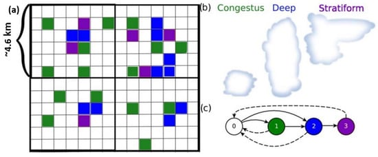
Figure 1.
(a) A graphic representation of the continuous-time Markov process on a microscopic lattice. The heavy grid lines represent a climate model gridbox and the colors represent varying states of the microscopic process. (b) Cartoon of the the cloud types associated with the cloudy microscopic states. (c) The transitions that are possible between the four states 0 to 3. Reproduced from [34] with permission.
The SMCM overlays a fine lattice on top of the computational grid box and associates a Markov process to each lattice site, i, deemed a microscopic cell (Figure 1a). Each process can, thus, take four different values according to whether the microscopic cell is occupied by a certain cloud type or not: (0) clear sky, (1) congestus, (2) deep, and (3) stratiform. In the case where the local interactions are ignored, these Markov processes are statistically independent and identically distributed. The transition probabilities from one state to another (Figure 1c) are obtained in terms of the infinitesimal (generator’s) transition rates , which depend on the following large-scale atmospheric variables or predictors.
- Convective available potential energy (CAPE): ;
- CAPE integrated over the lower troposphere: ;
- mid-troposphere dryness: , where is the equivalent potential temperature in the mid-troposphere and is a parameter whose value is given in Table 1.
 Table 1. Multicloud and atmospheric boundary layer (ABL) model parameters [42].
and are reference values for CAPE and dryness, respectively, whose specific values are given in Table 1.
The transition rates are based on intuitive rules according to observations of cloud dynamics in the tropics:
- A clear site turns into a congestus site with high probability if low-level CAPE is positive and the middle troposphere is dry;
- A congestus or clear sky turns into a deep convective site with high probability if CAPE is positive and the middle troposphere is moist;
- A deep convective site turns into a stratiform site with high probability;
- All three cloud types decay naturally to clear sky at some fixed rate;
- All other transitions are assumed to have negligible probability.
For brevity, the transition rates’ formulae, as introduced and used in [35], are listed in Table 2, where is an Arrhenius-type activation function: , if , and otherwise.
Table 2.
Transition rates are functions of the large-scale variables CAPE (C), low-level CAPE , and mid-troposphere dryness D, via the activation function defined in the text. The transition timescales are obtained from cloud simulation data based on a Bayesian inference technique [35].
The SMCM yields the cloud area fractions in each GCM grid box for each cloud type, , , and , that are given by the formulae:
where is the indicator function, which takes the value one if and zero otherwise. The cloud area coverage is used to control the strength and onset of convection, namely, by modulating the heating rates , , and associated with the corresponding cloud type (Figure 2). The precise formulae on how the cloud area fractions affect the heating rates are reported in Table 5.
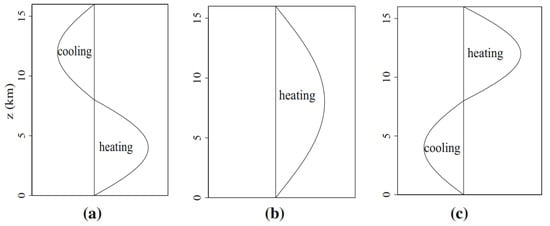
Figure 2.
Vertical profiles of heating and cooling associated with the three cloud types of the SMCM: (a) congestus, (b) deep convective, (c) stratiform. Reproduced from [42] with permission.
Because the processes are independent (as local interactions are neglected), the cloud area fractions form a multi-dimensional set of birth (clear sky site becoming cloudy), death (cloudy site becoming clear sky), and immigration (the fact that a given cloud type can transition to another type) processes. In this case, the birth, death, and immigration rates at any given time t are expressed (in closed form) in terms of the transition rates and the cloud area fractions at time t [35]. This is not the case when local interactions occur between microscopic sites, but acceptable approximations can be obtained under a mixing assumption [49]. Thus, when coupling the SMCM to a convective parameterization, the simulation of the full 2D microscopic lattice model is not necessary. Instead, only the (multiple population) birth and death processes for the cloud area fractions need to be evolved in time, over each climate model horizontal grid box, together with the large-scale climate model. This is achieved using Gillespie’s exact algorithm, and as such the whole stochastic cloud model adds a virtually negligible computational overhead to the parent model (e.g., [35,50]).
The following settings are chosen for the SMCM in the present study:
- lattice sites for each macroscopic/model gridbox;
- macroscopic grid box dimension = 4.59 km.
Accordingly, each microscopic/cloud site covers roughly an area of 150 m × 150 m. This is very high resolution in terms of representing multicloud dynamics, but nonetheless, the results obtained here do not seem to suffer from using the fine configuration. Although the fine model resolution is motivated by numerical stability and accuracy, it would be interesting to test the sensitivity to N in the future. For example, at the nearly 5 km resolution, a microscopic lattice as coarse as is physically conceivable.
2.2. The Simplified 2D Coastal Model
The dynamical core is based on the zonally symmetric Boussinesq and hydrostatic primitive equations on an f-plane. The main dynamical variables are the velocity (the zonal, meridional and vertical components, respectively), pressure p, and potential temperature . The two spatial dimensions, represented by y and z, are the meridional and vertical coordinates and time is denoted by the variable t. We assume a perfectly linear coastline that runs parallel to the equator. For convenience, the vertical coordinate is taken at the top of the ABL and the vertical scale is taken to be , where is the tropospheric height. The governing equations, in non-dimensional units, are [42]:
The forcing terms , , , and represent the sources and sinks of zonal and meridional momentum and potential temperature. In particular, includes heating and cooling resulting from convective and radiative processes. The term is the reference Coriolis parameter, which we assume fixed at some arbitrary latitude and which will be systematically varied as one of the main model parameters to study the dependence of coastal convection on f. The scaling factors used to adimensionalize the equations are summarized in Table 3 and rigid-lid boundary conditions on the vertical velocity are imposed at the top of the troposphere () and Earth’s surface () such that:
Table 3.
Troposphere model parameters and scaling factors [42].
Here, represents the ratio between the (fixed) boundary layer height and .
In addition to a linear coastline, we neglect the effects of orography. We also assume a homogeneous background with a constant stratification and an exponentially decaying moisture (water vapor) profile [36]. The equations of motion above are supplemented by a parameterization of deep convection that provides latent heating based on three prescribed heating profiles (Figure 2). The first is a half sine profile associated with deep convection and is set to heat the entire troposphere due to latent heat release from condensation associated with strong updrafts in cumulonimbus clouds. The second and third, associated, respectively, with congestus and stratiform clouds, are both full sine profiles that take opposite signs. Stratiform clouds heat the upper troposphere due to depositional growth within the stratiform anvils that lag the cumulonimbus and cool the lower troposphere due to the evaporation of stratiform rain below the cloud base, while congestus clouds warm the lower troposphere due to condensational latent heat release occurring within the congestus clouds and cool the upper troposphere due to longwave radiative cooling in clear air above the congestus and evaporation of detrained cloudy air at the top of the congestus cloud; see Figure 2. As a result, the deep convection heating profile forces the first baroclinic mode of vertical structure, while the congestus and stratiform heating and cooling profiles force the second baroclinic mode. This observation sets a lower bound on the vertical resolution of the model dynamics. Moreover, a constant and zonally uniform longwave radiative cooling is assumed. The ABL that lies below the trade wind inversion is assumed to be well mixed and non-stratified and to have a fixed thickness of 500 m.
Based on the assumed latent heating and cooling profiles, the first step for the numerical resolution of this model consists of projecting and truncating the free troposphere dynamics onto the barotropic and the first two baroclinic modes of vertical structure. The ABL dynamics are represented by a bulk (barotropic) system obtained from vertically averaging the primitive equations over the extent of the mixed boundary layer. More precisely, we set:
Here, and , for and , are the corresponding Galerkin truncation basis functions associated with the first and second baroclinic modes of vertical structure and for corresponds to the barotropic mode. The choice of the modes is linked with the heating profiles associated with organized convection in the sense that the first and second baroclinic modes are the modes that are directly forced by the latent heating, as already mentioned, while the barotropic mode appears to be the mode that responds directly to boundary layer convergence and surface pressure perturbations.
When the Equations (2)–(6) are projected onto the vertical structure modes above, we obtain three one-dimensional systems of PDEs that represent the barotropic and the first and second baroclinic mode dynamics, which are coupled to each other through the parameterized heating and cooling terms, projected advection nonlinearities, and boundary layer feedbacks. These equations are coupled to the bulk ABL equations through the convection parameterization and through the continuity of pressure and vertical velocity at the top of the ABL, which acts as an interface between the boundary layer and the free tropospheric flows. The details of the procedure are found in [39], and the resulting set of equations are reported in Table 4. In particular, we note that as a consequence of the ABL coupling, the vertical velocity at the top of the boundary layer is not zero and it induces a non-zero divergence of the barotropic component as can be seen in Table 4. The coupling via the continuity of pressure is reflected in the expressions of the barotropic and boundary layer pressures and near the top and bottom of that table, respectively. All forcing terms that appear on the right-hand side of the prognostic equations in Table 4, such as and that represent the radiative, convective, and turbulent mixing terms, are parameterized based on various physical assumptions and their expressions are given in Table 5. The interested reader is referred to [39,42] for further details.
Table 4.
Model equations. and are the meridional boundary layer transport operator and the barotropic transport operator, respectively. See [36,39,42].
Table 5.
Closure equations for convective and turbulent mixing forcing terms [42]. The primes indicate deviations from the radiative convective equilibrium (RCE) solution.
In Table 5 and elsewhere in the paper, for a scalar variable , we define , where the subscript t refers to values taken at the top of the ABL and b indicates bulk ABL values, while m corresponds to the middle of the troposphere. It is also worth noting that the first and second baroclinic components of pressure and vertical velocity flow from the projections of the hydrostatic balance and continuity equations.
To numerically solve the system of 13 1D equations in Table 4, a time-splitting method is employed [42]. The system is split into a conservative part, a hyperbolic part, and a nilpotent part that are each solved with their own appropriate numerical scheme for a better accuracy in key physical characteristics [51]. This scheme allows both numerical stability and accurate representation of key physical properties such as energy conservation and wave propagation characteristics [42]. A thorough description of the numerical method including its validation (with second-order convergence) is found in [42].
2.3. Model Setup
In order to simulate the dynamics of coastal convection as it interacts with the diurnal cycle of solar radiation, we consider a zonally symmetric coastal domain for which the coastline runs parallel to the equator and the land mass is located north of the coastline. The coastline latitude defines the center of the computational domain and it is used to set the reference Corioilis parameter . The model’s (meridional) resolution is set to grid points, which amounts to a mesh size km. The time step is set to s, which is a good compromise between obeying the Courant–Friedrichs–Lewy (CFL) condition for numerical stability and keeping a good accuracy and efficiency of the numerical simulation. The equations of motion are complemented with Dirichlet boundary conditions. The initial conditions are chosen to represent radiative convective equilibrium (RCE). RCE is defined as a space and time homogeneous solution of the coupled model equations. The details of the procedure used to construct a physical RCE solution for the SMCM model can be found in [39,52,53].
As already mentioned, one of the main goals is to assess the model’s ability to simulate features of coastal convection and see how these features change when the Coriolis parameter is changed systematically, especially in light of Rotunno’s theory [25] (see Introduction section), even though Rotunno’s theory is based on a linear model relying solely on dry boundary layer dynamics. As the Coriolis effect depends on the reference latitude , this task is tantamount to studying the evolution of coastal convection features for different values of the parameter . For this purpose, we run the model with the following values:
We note that is Rotunno’s critical latitude, where his theory breaks down. Simulations were run for each one of these latitudes for a long time period, exceeding 100 days, to reach a statistical steady state.
A key element of the model set up is that we impose a diurnal solar forcing over the land domain. In our code, the radiative forcing is included in the (discrete) gradients and , where and are RCE values and and are the variables through which we impose the diurnal forcing. The RCE values associated with the ocean part of the domain were determined in a previous study [42], but the ones associated with the land RCE are not known. We decided to impose the ocean RCE values both over the land and ocean domain and to run a first simulation of 100 days to reach a statistical RCE over the inhomogeneous domain. The model is then run for an extra 40 days and the corresponding simulation results are used in the analysis presented herein.
The ocean RCE values used as initial conditions are:
The main difference between the land and ocean parts of the model reside in the way the surface (latent and sensible heat) fluxes are imposed during the numerical simulations. For the ocean, we use only a constant surface forcing, which is consistent with its large thermal inertia. This is also consistent with Rotunno’s study [25]. To mimic the solar radiative forcing over the land part of the domain, we impose an additional surface forcing that follows a half-sine profile with time (Figure 3a) and that, for numerical stability, decays exponentially with latitude away from the coastline (Figure 3b,c). Namely, we set:
where is the distance from the coastline, from which the radiative solar forcing begins to fade, and is set to km. The latitude corresponds to the northern limit of the domain, where the additional forcing is set to zero. Moreover,
and
where , h, and with n being a whole number. The amplitudes and of the half-sine solar forcing are parameters that depend on the Bowen ratio.
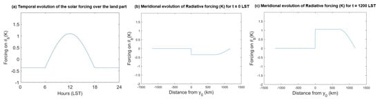
Figure 3.
Radiative forcing on : (a) temporal evolution over 24 h and spatial evolution at (b) 00:00 LST and (c) 12:00 LST, with y < 0: ocean, y > 0: land.
We introduce the parameters and that represent the normalized amplitudes of and , respectively. We have the relation , where is the Bowen ratio. Based on commonly observed values of diurnal sea surface temperature fluctuations in the tropics and subtropics, we impose K, which yields K, consistent with a Bowen ratio value of , corresponding to a relatively moist land such as a tropical forest, as indicated in Table 1. Since the effects of sensible and latent heat input from the surface on the atmospheric dynamics are very distinct (the first acting directly and primarily within the ABL and controlling dry convection, while the second is conditioned by the phase change of water and acts above the ABL), sensitivity analysis to is not considered in this study, though the results are not expected to be highly sensitive to as long as the latter stays relatively small.
3. Data and Methodology
3.1. The Raw Data
The time series of the root mean square (RMS) corresponding to the first 100 days of the simulation with the Coriolis parameter corresponding to the latitude are presented in Figure 4 for a few representative variables, namely, and .
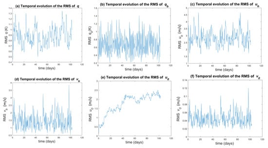
Figure 4.
100-day evolution of the root mean square (RMS) of: (a) q, (b) , (c) , (d) , (e) , and (f) for a coastline at latitude °.
After a transient period of roughly 10 days, all the variables except reach their statistical steady state around which they oscillate. The variable takes around 60 days to reach its statistical steady state.
The simulation is relaunched and rerun for another 40 days, starting from the solution at 100 days as the initial condition. The Hovmöller diagrams of selected variables are displayed in Figure 5 for these 40 days. We recall that land is and the ocean corresponds to . In the heating rates , , and plots, for example, various propagation patterns are visible. However, slower modes tend to occur over land and faster modes tend to occur over the ocean. The direction of propagation is both landward and oceanward. The moisture variables also appear to have slow and fast streaks propagating in both directions. The presence of different and entangled propagation patterns with different speeds of propagation makes the analysis complex and no general conclusion can be made at this point. To more easily distinguish and individually analyze these patterns and what they represent physically, we use a spectral or Fourier transformation on the variables y and t in the next sections.
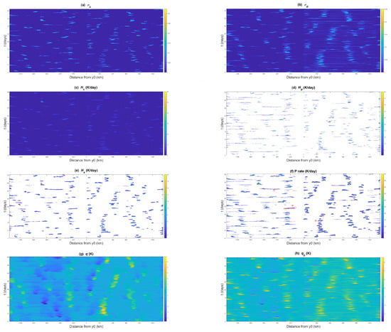
Figure 5.
40-day Hovmöller diagrams: (a) , (b) ,, (c) , (d) , (e) , (f) precipitation, (g) q, and (h) for a coastline at latitude °. Examples of slow mode and gravity wave signals are depicted in (d), denoted with letters Sl and G, respectively. The line labeled St denotes a nearly standing slow mode that modulates the diurnal mode. The diurnal mode is evidenced by the precipitation events embedded within the nearly standing slow mode, occurring every day from day 4 to day 12. There are exactly 9 within the first 9 days of the slow mode signal.
As depicted on the precipitation contours in Figure 5f, three modes of variability seem to dominate our simulations: the diurnal mode, which is the direct response to the diurnal solar forcing; slowly propagating mesoscale rain bands that can cross the coastline in either direction and have life spans of two days or more; and fast propagating gravity waves. Examples of the gravity wave and slow modes are marked in Figure 5f by oblique line segments labeled by the letters G and Sl, respectively. The slopes of these lines define the average propagation speed of these wave-like signals and are roughly 30 ms and 4 ms for the gravity wave (G) and slow (Sl) modes, respectively. The line labeled with St denotes a nearly standing slow mode that modulates the diurnal cycle. The presence of exactly 9 precipitation peaks within the first 9 days of the marked nearly standing slow mode event is evidence of the diurnal mode. The same modes are also visible on the contours of all the other thermodynamical variables depicted in Figure 5 and in particular those of the cloud area fractions and and moisture q and . Although not shown here, the same is valid for and the flow velocity variables as well as pressure and temperature.
The modes of variability are, thus, grouped hereafter into three categories: the diurnal mode, the slow modes, and the gravity wave modes. The slow modes typically have frequencies less than 1 cycle per day (cpd), while the gravity wave modes have frequencies larger than 1 cpd. It is worth noting that orographic effects are neglected in the present model, so all the gravity wave signals are solely driven by the differential heating between the land and ocean parts of the domain or by convective heating events.
3.2. Spectral Analysis
In order to single out and individually analyze the three modes of variability identified above, we will use the Fourier transform. For each given mode, we choose a variable that will serve as a reference for the filtering process, typically the one that appears to carry the strongest spectral signal. For the diurnal and gravity wave modes, is chosen as the reference, as these modes appear to be dominated by fluid dynamics (namely the sea and land breeze for the diurnal mode and divergence for the gravity wave modes), while for the slow mode we choose precipitation P as the reference variable.
To separate the part of the flow that is associated with the diurnal mode, for example, we created a filter that we apply to each one of the 24 variables in the spectral domain. That filter is created using the spectral field as a reference. It consists of a matrix of the same dimension as the field, whose coefficients are null except for a rectangle centered around the peak of interest corresponding to the diurnal mode, namely, a box composed of four-by-four pixels in the spectral domain, centered around the point with wavenumber and frequency cpd. Once the variable is filtered, the next step is to transform it back into the time and space domain with an inverse Fourier transform.
To filter the gravity wave, we use the same process on the field with the same type of filter as the previous one, but with a rectangle of 1-coefficients around the peak of interest at frequency (cycles per day) and wavenumber . In our model, the 1st and 2nd baroclinic modes, with respective reference gravity wave speeds ms and ms [50], are nonlinearly coupled through advective nonlinearities, the barotropic mode, boundary layer dynamics, and latent heating. This coupling results in a modulation of all the gravity wave speeds generated in the model by both the 1st and 2nd baroclinic wave speeds. As such, the gravity waves in our system, which are typically coupled to both the moist thermodynamics and those four dynamical modes, can have wave speeds ranging anywhere between zero and 50 ms and higher. In our study, we only select one gravity wave to exhibit the typical behavior of these waves. To be able to determine a general behavior for the gravity waves of this model we would need to study all of them, but we deemed it more interesting to focus more attention on the diurnal mode, which carries the majority of the sea and land breeze effects.
For the analysis of the slow modes, a single (slow) mode propagating oceanward is selected. It corresponds to a spectral peak centered around the point in the spectral domain plot (not shown). It is worth noting at this point that a more efficient and systematic way to estimate the average propagation speed of a wave-like signal using the spectral diagram is to simply divide the frequency by the wavenumber of the corresponding spectral peak.
4. The Physical Features of the Main Modes of Variability in Coastal Convection
Our analysis below revealed that the diurnal mode is strongly modulated by slowly moving MCSs and heavily affected by the Coriolis force. The latter effect makes the dynamical fields of the diurnal mode switch from hyperbolic wave-like morphology at low latitudes to elliptic patterns at higher latitudes, roughly above 30 degrees, consistent with Rotunno’s linear theory [25]. In particular, the morphology of and interaction between dynamics, moist thermodynamics, and cloud fields are investigated in detail.
Not surprisingly, the diurnal cycle is found to be the fundamental mode of variability that controls the back and forth switching between the sea and land breeze characterizing the surface winds across the coastline and associated return flow aloft, leading to upward motion and convective activity over land (ocean) during sea breeze (land breeze) periods, consistent with observations in many respects [54]. The details, however, are sensitive to the Coriolis force as the dynamical response switches between hyperbolic and elliptic behavior. The comparison of the onset of sea and land breeze to existing observations are mixed between being somewhat off in the deep tropics to showing a higher degree of consistency at higher latitudes [29,54,55,56,57,58,59]. Although it follows more or less of a similar pattern as a function of the Coriolis force, the extent of the penetration distance of the sea and land breeze is found to be more consistent with observations in our nonlinear and highly more complex and more realistic model than in Rotunno’s linear theory [9,25,29,60,61]. Moreover, the results demonstrate that the diurnal mode alone does not by itself represent the whole complexity of coastal convection. Instead, high-frequency modes, consisting mainly of fast-moving gravity waves and slower-frequency modes, reminiscent of mesoscale convective systems, contribute significantly to the variability in coastal convection, and all three provide comparable amounts of precipitation [62,63].
4.1. The Diurnal Mode
Slow Modulation and Transition from Hyperbolic to Elliptic Behavior
The top row of Figure 6 plots the time evolution of the (filtered) diurnal mode for mid-level moisture q, boundary layer moisture , and deep convective heating during the last 40-day simulation at 10° latitude near the coastline (). The diurnal oscillations appear on top of much slower oscillations, which act as large-scale envelopes that modulate the diurnal mode. The period of these envelopes ranges from 10 to 40 days and seems to vary depending on the latitude of the coastline (results not shown).
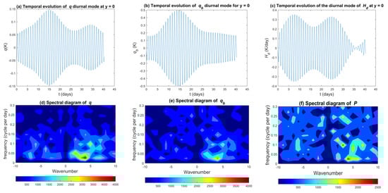
Figure 6.
Top: Temporal evolution of the diurnal mode of (a) mid-tropospheric moisture q, (b) ABL moisture , and (c) deep convective heating . Bottom: spectral diagrams of (d) q, (e) , (f) surface precipitation P for a coastline latitude of °, focusing on low-frequency modes highlighting the existence of nearly standing slow modes that tend to modulate the diurnal mode.
The bottom row of Figure 6 displays spectral diagrams of mid-tropospheric and boundary layer moisture q and , and of surface precipitation P. For q, two peaks are noticeable at and . These peaks correspond to modes with periods of 14 and 20 days, respectively, which match the modulation periods of the diurnal modes reported earlier and favors the hypothesis of a modulation by nearly standing slow modes. The same peaks are also visible in and P. Although interesting, we defer the discussion of the nearly standing slow modes for a future study to focus more on the dynamical and morphological structure of the diurnal mode and try to draw attention to the similarities between our simulations and previous observational and theoretical studies. We are particularly interested in the variation in these features when the coastline latitude (or equivalently the Coriolis parameter) is varied and how our results compare to Rotunno’s theory [25].
Figure 7 shows the (daily) composite Hovmöller diagrams of the diurnal mode for the meridional velocity in the ABL averaged over the 40 days of the simulation and for several coastline latitudes, ranging from 0 to 40°. Positive values represent southerly winds (i.e., from ocean to land) and negative values represent northerly winds (i.e., from land to ocean). For tropical latitudes (°), the contours consist of angled streaks, suggesting that the sea breeze propagates in a wave-like pattern along two ray paths that are extending from both sides of the coastline, while at higher latitudes the contours display nearly elliptical patterns. This is consistent with the theoretical results of [25] discussed in the Introduction section. In particular, Rotunno’s theory predicted that for , the model equations governing the diurnal sea and land breeze response are hyperbolic and the solution is given by a superposition of inertia–gravity waves propagating away from the coastline.
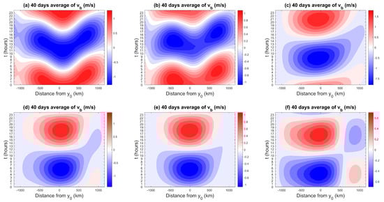
Figure 7.
Composite daily Hovmöller diagrams of the diurnal mode of v at z = 336 m for coastline latitudes at (a) 0°, (b) 10°, (c) 25°, (d) 30°, (e) 35°, and (f) 40°.
Nonetheless, there are some noticeable differences between the purely linear and dry solution of Rotunno and the present simulations. In the purely linear theory, the wave dispersion formula is given by , with and the horizontal and vertical wavenumbers, respectively. As noted in [64], energy propagates along ray paths, following the group velocity according to the equations: , where A is a constant. So, in the -plane, wave energy propagates along ray paths of constant slope. For , making , and energy is propagating southward, whereas for , and energy is propagating northward. There are, thus, two ray paths intercepting each other at the coastline . However, the ray paths in Figure 7 do not intercept exactly over the coastline but over a latitude a bit shifted to the north of the coastline. This qualitative mismatch between the linear theory and the present simulations may be due to the fact that our model is highly nonlinear. Unfortunately, observational data in this respect are lacking to be able to decide which behavior is more physical.
As the latitude becomes closer to the threshold latitude °, the ray paths flatten (e.g., Figure 7c). At 30° and above, the ray paths disappear and the sea/land breeze flow is no longer propagating as a wave but just moves between the land and ocean domains. Based on Rotunno’s theory [25], in the mid-latitudes (), the linear model equations are no longer hyperbolic but become elliptic when the ° threshold is crossed, and the sea breeze flow response no longer follows a ray path but instead exhibits an elliptical flow pattern that flows landward in the lower atmosphere and back to the ocean in a return flow aloft. This is consistent with the time–latitude contours in Figure 7d–f that do not suggest wave propagation. However, many fine details emerge from our simulation that are different from basic ray paths versus elliptic flow patterns. In Figure 7f with , for instance, instead of one simple pattern consisting of oscillating northerlies and southerlies as in Figure 7c–e, we have a quadrupole v structure suggesting divergence/convergence occurring near the middle of the land domain. This amounts to a reinforcement and perhaps a further southward shifting of the upward motion over land during the sea breeze phase when the Coriolis force is increased, which is explored further in the next section.
4.2. Dynamical and Thermodynamical Structure of the Diurnal Mode
In Figure 8 and Figure 9, we plot time-averaged contours in the meridional–vertical () plane for the three velocity components, temperature, latent heating, and pressure for the cases and , respectively. We also plot the mean mid-tropospheric moisture as a function of y on top of the heating contours, while the velocity arrows are overlaid on top of the remaining panels. For the case °, Figure 8b shows the sea breeze peaking in the lower troposphere, with maximum speeds of 1.2 ms. In the upper troposphere, there is a weaker return flow. The equivalent figure for the land breeze (not shown) has similar maximum speeds even though observations indicate that the land breeze is often weaker than the sea breeze [54]. The effect of the Coriolis force is visible in Figure 8a, where the zonal velocity is positive in the lower part of the free troposphere, which is the sign of an eastward flow, consistent with the Northern Hemisphere location. Because 10° is still close to the equator, the intensity of the Coriolis force is low, hence the weak wind deviation as u reaches values of only up to ms, which is much smaller than the maximum v value. The vertical velocity in Figure 8c is 100 times weaker than the maximum horizontal wind speeds and displays an antisymmetric pattern with respect to the coastline. On the land side, there is weak downward motion close to the coast followed by significantly stronger and deeper upward motion farther inland. The opposite pattern is seen on the ocean side. The combined action of v and w creates two small counterclockwise flows on each side of the coastline that are surrounded by a bigger counterclockwise flow centered at the land/ocean interface.
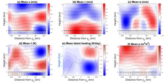
Figure 8.
40-day average vertical cross sections of (a) u, (b) v, (c) w, (d) , (e) latent heating and the free tropospheric moisture perturbation (dark line), and (f) p at sea breeze peak time, 02:00 LST for °. The arrows depicts the flow pattern.
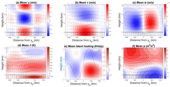
Figure 9.
40-day average vertical cross sections of (a) u, (b) v, (c) w, (d) , (e) latent heating and the free tropospheric moisture perturbation (dark line), and (f) p at sea breeze peak time, 18:00 LST for °. The arrows depicts the flow pattern.
Figure 8e shows strong heating aloft and strong cooling at lower levels over land, indicating persistent stratiform heating. The mid-troposphere (vertically averaged over the free troposphere—above the ABL; see [39]) moisture peaking in the middle of the land domain is consistent with the evaporation of stratiform rain represented by the term in the downdraft mass flux (See Table 5), though a thorough moisture budget analysis is needed in order to quantify the relative contribution of this term compared to other processes such as low-level convergence and mesoscale downdrafts. The lack of convection over the ocean means that the weaker, but persistent, longwave radiative cooling becomes dominant throughout the troposphere. The reverse heating field during the land breeze (not shown) is a strong congestus signature over land (i.e., cooling aloft and heating at lower levels; see Figure 2) and a weak deep convective signature over the ocean (i.e., heating throughout the troposphere with a mid-tropospheric maximum). In this situation, convection over the land is forced by enhanced surface heating but limited in vertical extent by the descending motion associated with the land breeze circulation, while deeper convection over the ocean is supported by the low-level convergence and ascending motion.
In the sea breeze phase, the pressure field (Figure 8f) exhibits upper-tropospheric positive anomalies, whereas the lower troposphere has weaker negative anomalies throughout the ocean domain and extending to up to 500 km inland. Above this penetration level (near 500 km), the pressure field displays positive anomalies in the mid-troposphere and negative anomalies aloft and below. This pressure pattern is consistent with the structure of the zonal velocity in this region of the domain, where it exhibits a double jet shear with westerly winds in the mid-troposphere and easterly winds in the lower and upper troposphere. In addition to complying with the hydrostatic balance relation, the perturbation of the potential temperature distribution over land in Figure 8d shows negative in the ABL because of the negative solar forcing imposed at 02:00 LST. In the lower free troposphere, the anomaly is positive and becomes negative in the upper troposphere. The structure is reversed over the ocean. This means that warm air is raising from the lower troposphere and cold air is sinking from above, consistent with a convective flow.
Figure 9 shows the same variables at the time of the maximum sea breeze magnitude for when the coastline is set at °. Except for the major geometrical differences in the flow patterns, with wave-like tilted meridional wind patterns at 10° and more elliptical patterns at 35°, reminiscent of Rotunno’s theory, many similar physical features can be discerned between the latitudes. Figure 8b and Figure 9b show consist landward flow in the lower troposphere as a continuation of the sea breeze in the ABL that penetrates to roughly 5 km high, followed by a similar return flow in the upper troposphere. Furthermore, the sea breeze (v in the ABL) intensities reach comparable maxima of up to 1.2 ms and slightly higher. Consistently, the free tropospheric v values also exhibit comparable ranges of intensities varying between ms for the landward flow in the lower troposphere and ms for the return flow in the upper troposphere. Nonetheless, the geometry of the two flows is fundamentally different, as already mentioned. Importantly, the v contours in Figure 8b present tilted structures in the free troposphere, the landward (positive) flow exhibiting a pair of maximum values located on either side of the coastline () and a minima triplet of the return flow (negative v), one of which is located near the coastline. The v contours in Figure 9b on the other hand present exactly one maximum and one minimum. The first being located at the ABL–lower troposphere interface, and the second at three-quarters of the height of the troposphere.
Moreover, the Coriolis force effect appears to be stronger at 35° as the zonal velocity values in Figure 9a reach maxima/minima of ms, while in Figure 8a, the zonal velocity values do not exceed ±0.25 ms. This is despite the fact that the corresponding meridional flows (the sole momentum source for the zonal velocity, through the Coriolis effect) have comparable values. However, consistent with the geometrical differences in the corresponding v flows, the u flows also have some considerable differences. While the contours in Figure 8a present a strong asymmetry with respect to the coastline, the ones in Figure 9a have a nearly symmetric structure, with one major double jet shear centered at the coastline, consistent with the v flow patterns in Figure 9b.
Not surprisingly, the vertical velocity contours in Figure 8c and Figure 9c have the same overall upward motion over land and downward motion over the ocean. The air that is brought to the land by the sea breeze rises to the higher troposphere and then moves oceanward via the return flow. Due to the geometrical differences, mentioned several times now, at 35, the combined action of v and w creates one large counterclockwise flow spanning the entire depth of the troposphere centered over the interface between the land and the ocean, which is fundamentally different from the equivalent flow pattern at 10, which consists of multiple cells.
Fundamentally different from the case, the latent heating contours in Figure 9e suggest that over land, where the convection takes place, there is a mix of congestus and deep convective clouds because of the larger mid-tropospheric heating compared to the relatively smaller upper-tropospheric cooling. Recall that at 10, the heating field over land is dominated by upper-level heating and lower-level cooling, which is the complete opposite of Figure 9e. Over the ocean, there is a bottom-heavy cooling and weak upper-tropospheric heating, a signature of stratiform rain systems, that tend to overcome the imposed uniform radiative cooling there, which is somewhat similar to what we have observed in the 10 case.
Anomalies of at 35 are positive in the lower troposphere and ABL, across both the ocean and land domains, and become slightly negative in the upper troposphere over land (Figure 9d). The pattern is consistent with the latent heating structure over land, but less so over ocean. Figure 9f shows stronger low-level negative pressure anomalies compared to the tropical case but similar high-pressure anomalies in the upper troposphere. These patterns are also fundamentally different from what is displayed in Figure 8d,f.
4.2.1. Sea and Land Breeze Initiation and Peak Times, and Physical Mechanisms of the Diurnal Mode
Using Hovmöller diagrams, such as the ones in Figure 7, for the meridional velocity (not shown), it is possible to determine when the sea and land breezes begin and when they reach their greatest strength. Figure 10 shows the average starting time and the average time of peak magnitude of both the land and sea breezes at the land–ocean interface, averaged over the last 40 days of the simulations, for different latitudes. At the equator (°), the model’s average sea breeze starting time is 17:00 LST near the coastline. This early evening start time is obviously unphysical since sea breezes are observed to begin much earlier in the day in the tropics, as it is the land breeze that begins setting up as the sun sets. However, this large time offset was also observed in Rotunno’s model [25]. This mismatch could be, therefore, associated with the idealized boundary layer setting that produces an overly long lag between when the sun rises or sets and the response of the land temperature. Some tuning is perhaps required in order to obtain the right timing of the sea breeze onset. It is also possible—though not clear how—zonally propagating waves and synoptic-scale dynamics, which are not represented in the zonally symmetric setting, may play a role in determining the sea/land breeze onset near the equator. Moreover, for a coastline located at °, the modeled tropical sea/land breezes in Figure 7 have maximum speeds of ms, which are smaller than the values of 3 ms found in [29] using ERA5 data off the west coast of Sumatra (°), but the two speeds remain comparable. It is, thus, perhaps fair to say that models with zonally symmetric and/or idealized/bulk boundary layer dynamics fail in capturing the correct timing of the sea and land breeze near the equator, even though the reason is still unclear!
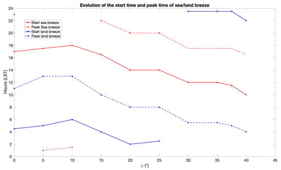
Figure 10.
Evolution of the start and peak times of the sea and land breezes for different coastline latitudes.
As the latitude increases, the sea breeze starting time increases slightly to 18:00 LST near ° and then decreases monotonically to about 10:00 LST at ° (Figure 10), which is more consistent with physical expectations. The same behavior is observed for the starting time of the land breeze, which begins around 4:30 LST when ° (again, unphysical and maybe an artifact of the modeling framework; typical land breezes begin in the early evening as mentioned previously), is 6:00 LST near °, and drops monotonically to 22:00 LST at °. It is not clear at this point whether this systematic regression with latitude/Coriolis parameter of the sea and land breeze onset time is observed in nature, as various environmental conditions, especially synoptic wind and ocean dynamics, seem to affect this timing [55,56].
Nonetheless, for °, the model’s sea breeze starting time near the coastline of roughly 14:00 LST is in agreement with observations of a sea breeze near the coastline of Abu Dhabi (roughly ° N) starting some time between 13:00 and 14:00 LST [57]. A similar onset time, near 14:00 LST, was reported at Perth, Australia (∼32° S) [58], while [59] reported a sea breeze onset time around 09:30 LST for the Korean coastal region of Boseong (° N). The latter may be due to topographical effects associated with the proximity of the Goheung-eup Peninsula on the ocean side of the coastline.
The overall regressing tendency is singular and can be partly explained by the Coriolis effect that is null at the equator and increases as the latitude increases. Indeed, the meridional and zonal velocities in the ABL ( and ) are linked by two equations (the and equations in Table 4) in a way that each of the variables modulates the evolution of the other through a term that depends on the Coriolis parameter . This is a well-documented phenomenon through which the Coriolis force affects the sea and land breezes by redirecting the surface winds to blow at an angle with respect to the coastline [65]. This also may explain why the zonal symmetry framework can be a problem for obtaining an accurate account of the sea and land breeze evolution at (near) the equator where the Coriolis force is zero, to the point that the true evolution of the zonal flow is (almost) completely absent.
Figure 11a–c allow a closer examination of the coupled evolution of and , as well as the pressure perturbation in the ABL, for different latitudes. At the equator, the Coriolis force is null, so has no forcing and stays null at all times, so is only modulated by the term. Away from the equator, we can see that is preceding and that the de-phasing is evolving with the latitude. The de-phasing between and seems to stay constant no matter the latitude. Figure 11d represents the evolution of the de-phasing between and with latitude. The de-phasing increases rapidly when the latitude becomes greater than ° as the Coriolis force becomes more intense. This de-phasing stabilizes at ° until °, where it starts to slowly decrease. While this de-phasing is driven in large part by the Coriolis force, the fact that it is not monotonically changing with latitude suggests that it may also depend on feedback factors such as boundary layer coupling with free tropospheric dynamics, which is in turn directly coupled with convection and boundary layer friction through the terms and ( and ) in the () equation.
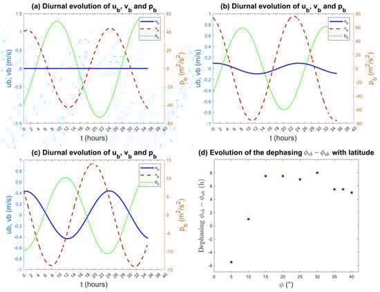
Figure 11.
Evolution of the diurnal modes of , , and during 36 h for the coastline latitudes (a) 0°, (b) 10°, and (c) = 35°, and (d) evolution of the de-phasing with the latitude.
As observed in other studies [9,60], the diurnal mode also seems to be driving the off shore migration and in-land penetration of coastal deep convection and the associated precipitation. In Figure 12a–e, Hovmöller diagrams of the diurnal precipitation anomalies are plotted for different coastline latitudes. If we focus on the coastal area and put aside the far ends of the domain that are more directly influenced by the artificial boundary conditions, for high enough latitudes (), the main behavior of the diurnal precipitation anomalies seems to suggest a pattern that is consistent with an early morning initiation stage over the ocean, a mature stage, where precipitation first peaks over the ocean around 09:00 LST, and then a landward propagation followed by a secondary peak over land itself in the late afternoon to early evening. For 0° (Figure 12a) and 5° (not shown), the precipitation initiates over the land and ocean simultaneously, and propagates oceanward in both cases with a phase speed of ms over land and ms over the ocean, with a weaker intensity for precipitation over the ocean. For the latitudes 10° to 30°, the precipitation also initiates over both the ocean and land and propagates both landward and oceanward with phase speeds around ms. These speeds are roughly in agreement with various datasets of offshore rainfall migration speeds for the global tropics, that have been found to range from 3 to 20 ms [29]. For 35° to 40°, the precipitation propagates landward only, with a phase speed of roughly ms.
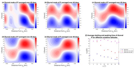
Figure 12.
40-day composite Hovmöller diagrams of the diurnal mode of precipitation for a coastline at (a) 0°, (b) 10°, (c) = 25° and (d) = 35°, and (e) = 37.5°, and (f) average starting/peaking time of the precipitation over land and ocean for all the studied coastline latitudes.
Figure 12f shows the starting time of the precipitation as well as the time of peak precipitation magnitude over the land and ocean domains for all the studied coastline latitudes. For virtually all latitudes, precipitation is initiated over the ocean during the night or early morning (between midnight and 08:00 LST). This is in agreement with [34], who reported that in the maritime continent (i.e., the Indian Ocean/Western Pacific warm pool region), rain is concentrated over the oceans between 21:00 LST and 09:00 LST. For coastline latitudes below 20°, albeit away from the coastline, the precipitation peaks in the afternoon from 14:00 LST to 19:00 LST over the ocean, which differs from observations of oceanic precipitation that show peaks in the early morning [34]. For latitudes above 20°, the precipitation peak over the ocean varies between early to late morning hours (4:00 LST to 11:00 LST). The precipitation peak over land occurs during the late afternoon/evening (17:00 LST to 20:00 LST) for all the simulated latitudes, which is in agreement with the land-side coastal regime observed in [66], that is characterized by precipitation peaking at 18:00 to 00:00 LST. However, for 0° (Figure 12a) and 5° (not shown), which would be classified as a seaside coastal regime according to [66], the evening peak time over land differs from observations that show precipitation peaking at 03:00 to 12:00 LST.
4.2.2. Sea and Land Breeze Penetration
Another important feature of the sea/land breeze is its flow penetration landward and oceanward. The penetration of the sea (land) breeze is defined as the distance between the coastline and the breeze front over land (the ocean). To define the sea and land breeze front position with precision, we use the low-level convergence method (e.g., [29]), which in the present setting associates the sea/land breeze penetration front with the first point of maximum divergence/convergence in the ocean/land closest to the coastline. Figure 13a–e show the Hovmöller diagrams of the ABL convergence () for different latitude cases. Consistent with the wind patterns in Figure 7, the near-surface convergence patterns also undergo a transition between wavy-like patterns for latitudes below the 30° critical threshold to elliptical patterns beyond this value. It is also worth mentioning that the most significant regions of convergence and divergence in Figure 13a–e are somewhat correlated with the corresponding positive and negative precipitation anomalies in Figure 12. However, unlike certain models, such as those based on a moisture convergence closure, positive convergence is not always associated with positive precipitation anomalies. A good example is given by the case , which shows a strong convergence–divergence dipole over the ocean in Figure 13a, but the associated precipitation patterns in Figure 12a are very weak and appear to be negatively correlated.
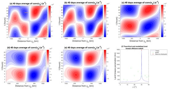
Figure 13.
Hovmöller diagram of the meridional convergence of for a coastline of latitude (a) 0°, (b) 10°, (c) = 25°, (d) = 30°, and (e) 35° during 24 h, and (f) comparison between the land breeze penetration predicted by Rotunno’s theory and the modeled one. The land breeze penetration for the coastline at 30° is marked by a red star because it is not predicted by Rotunno’s theory. The line segment in (a) connects the shoreline with the first point of maximum convergence over the ocean and marks the distance of the land breeze penetration.
At °, the convergence contours show streaks propagating offshore at a speed of roughly ms (Figure 13a). This is about three times larger than the propagation speed of the convergence at 975 hPa reported by [29] near the west coast of Sumatra, who estimated convergence propagation speeds from ERA5 that ranged from 5 to 6 ms depending on the season. However, given that many factors are not accounted for in the model that can influence the land breeze propagation speed (especially at and near the equator as has been already stressed), the modeled values are encouraging as they are near the same order of magnitude.
Figure 13f compares the modeled land breeze offshore extent, measured by the distance of the first point of maximum convergence from the coastline, to Rotunno’s theory as a function of latitude. For small latitudes (below 15°), the behavior of the modeled land breeze penetration stays almost constant around 200 km. From 15° to 25°, the offshore extent mainly increases monotonically as expected by Rotunno’s theory, except for the surprisingly high value of 800 km at 15°. It is hard to tell what is happening in this case and further investigations are warranted. From 30° to 40°, the land breeze penetration seems to stabilize around 400 km or slightly decreases as in Rotunno’s theory, but the number of sampling points (simulation cases) is too small to warrant a definitive conclusion.
It is also worth mentioning that the penetration distances (based on the convergence method) predicted by our model are larger than the values predicted by Rotunno’s theory. The land breeze offshore extent varies between 60 km and 130 km in the linear theory while our model produces values between 165 km and 800 km (Figure 13f). Rotunno’s model is in many respects more idealized compared to the model used in this study, which makes the difference between the model and the theory unsurprising. For example, Rotunno’s model is linear and deals only with boundary layer dynamics. Our model is nonlinear and is fully coupled to the upper free troposphere dynamics and to moist physics. Further investigation is needed in order to understand what causes these and other discrepancies. However, some of the values predicted by our model are consistent with observations of land breeze penetration. For example, [61] reported that mean offshore land breeze penetration is around 300 km at 30, similar to our model, although they found that penetration decreases to about 100 km above 40. Moreover, our model’s land breeze penetration for the 0° to 10° latitudes are also consistent with [61], who found that the influence of land extends several hundred kilometers from the shore in the tropics.
4.3. Fast and Slow Modes
In this section, we briefly examine some of the most salient physical features of the (moist) gravity wave and slow modes of coastal convection identified from the coastal SMCM simulations. We only focus on one characteristic gravity wave mode and one characteristic slow mode to ease the comparison between the different latitude cases. We selected the gravity wave with frequency cpd and wavenumber that is propagating oceanward in each latitude case. Figure 14 shows the Hovmöller diagrams of the gravity wave mode precipitation anomalies for different coastline latitudes. Precipitation initiates over the land part of the domain during the night (00:00 LST on average) and in the middle of the day (12:00 LST) and then propagates offshore. The propagation sometimes seems to be split into two phases, with two different speeds of propagation over land and the ocean (Figure 14c) or with a discontinuity between the propagation over land and the ocean (Figure 14b).
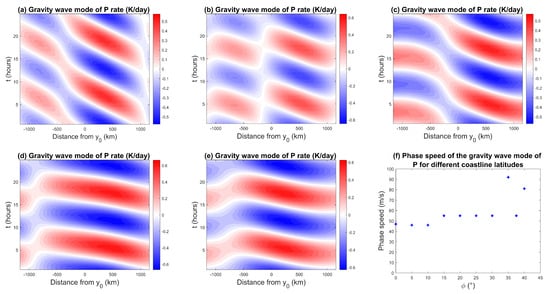
Figure 14.
Hovmöller diagram of precipitation for the gravity wave mode for a coastline at (a) 0°, (b) 10°, (c) 25°, (d) 35°, and (e) 40°, and (f) evolution of gravity wave speed by coastline latitudes.
The rainfall propagation speed plotted in Figure 14f stays relatively constant with latitude at about 50 ms, except for surprisingly high values up to ms for the 35° and 40° cases. In theory, because the gravity waves generated in the model are modulated by both the first and second baroclinic modes, we expect phase speeds that are between ms and ms [50]. However, due to convective coupling we observe higher values. This behavior is somewhat unexpected and perhaps unphysical and, thus, merits further investigation in the future. Though it is worthwhile mentioning that excessively large phase speeds of (linear unstable) moist gravity waves have been observed in models for convectively coupled waves [67]. The moisture in the free troposphere is also carried by gravity waves, and Hovmöller diagrams of the moisture perturbation (not shown) indicate generally similar patterns and propagation speeds as the precipitation.
Observations have shown that coastal and diurnally forced precipitation events are also driven by slower modes of propagation associated with mesoscale convective systems (MCSs) [62,63]. MCSs are the largest of the convective storms, often containing large stratiform rain regions in addition to the prerequisite organized deep convection, and are responsible for a large part of the precipitation observed in the tropics [45]. Figure 15 shows the Hovmöller diagram of the precipitation associated with the oceanward propagating slow mode of period 5 days for different latitudes. The offshore rainfall propagation speeds are plotted in Figure 15f. The phase speeds average 2.8 ms in the tropics and reach 3.85 ms for °. These values are slightly underestimated but remain on the same order of magnitude when compared to migration speeds of 5 ms observed for MCSs in the maritime continent for a coastline of latitude −6° [62].
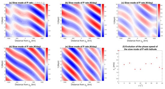
Figure 15.
Hovmöller diagram of precipitation for the slow mode for a coastline at (a) 0°, (b) 10°, (c) 25°, (d) 35°, and (e) 40°, and (f) evolution of precipitation phase speed by coastline latitude.
Relative Precipitation Contributions
As we saw previously, different modes of variability drive the precipitation over our coastal domain. It is of paramount importance, both for theoretical understanding and for forecasting purposes, to be able to establish the relative contributions of each one of these modes to the total precipitation in coastal areas. For that purpose, we filter the precipitation data to separately study these modes. For simplicity, we divide the spectral domain into fast modes, slow modes, and the diurnal mode categories, where frequencies above 1 cpd are grouped in the fast mode category and frequencies below 1 cpd are grouped in the slow mode category. Examples of slow, diurnal, and fast mode precipitation events are highlighted in Figure 5.
The precipitation time series are filtered using a spectral cut-off filter to separate the diurnal, fast, and slow modes of precipitation according to the definition above. Although not shown, the raw spectral power plot shows that the most powerful peaks in the spectrum are among the slow modes of variability. The second most powerful peak is associated with the diurnal mode and the weakest peaks correspond to the fast gravity wave modes. Although, the slow and fast modes exhibit multiple spectral peaks, while the diurnal mode has only one relatively narrow blob concentrated near the spectral point and cpd.
The left column of Figure 16 displays the first 10 days of the simulation of the precipitation generated by each one of the filtered groups summed over the latitude at three coastline latitudes, while the right column displays the spatial RMS of the precipitation for each mode. Despite the differences in the spectral power peaks, the diurnal, slow, and fast modes produce precipitation of similar intensities (Figure 16a,c,e). Even though the fast mode’s peak intensities appear to be weaker when taken separately in the raw spectra (not shown), there are so many of them that their summed contribution becomes comparable to the intensity of all the slow modes together and the diurnal mode alone.
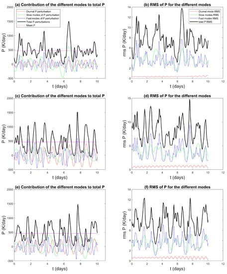
Figure 16.
10-day time series of the precipitation and precipitation RMS decomposed by mode for (a,b) , (c,d) , and (e,f) .
The RMS time series in Figure 16b,d, and f indicate that the variability in the gravity modes is the largest and that in the diurnal mode is the smallest. This suggests that the diurnal mode is very predictable, as expected, while the slow and fast modes display relatively stronger variability making their behavior somewhat stochastic. We note that the RMS of the total precipitation seems to be more often closer to the RMS of the fast mode precipitation (Figure 16b,d,f), thus the predictability of coastal convection could be mostly affected by gravity wave dynamics that may be significantly contributing to the high-frequency precipitation signals, as in Figure 14, which are often poorly represented in climate and weather prediction models.
As shown in Section 4.1, the diurnal mode is modulated by the slow modes, and thus, its amplitude varies with time. The stronger its amplitude, the stronger its relative influence on the total precipitation will be. In Figure 16c, we see an example of such modulation. The amplitude of the diurnal precipitation is small at the beginning of the 10 days and increases with time to become of the same order as the amplitude of the fast and slow modes.
Furthermore, a technical point worth noting is related to the sampling of the fast modes. Because the time interval between successive model outputs is approximately 1 h, the sampling of the fast modes turns out to be an issue. The fastest of these modes evolves very quickly and would require smaller time steps to represent them accurately. This under-sampling generates large positive and negative peaks in the temporal evolution of the fast modes of precipitation. These peaks degrade the accuracy of the total sum calculated and can also cause negative values for the total precipitation (which are not physical). To solve this issue, a smoothing function was applied to the precipitation fast modes to lessen these peaks and provide more realistic time series of the precipitation associated with the fast modes, as shown in Figure 16.
5. Conclusion
In this paper, we used a zonally symmetric model to simulate coastal convection over a simplified coastal domain consisting of a land part and an ocean part separated by a coastline that runs parallel to the equator and is located at a fixed latitude. The model was originally developed for the zonally symmetric dynamics of the monsoon and Hadley circulations [42]. In particular, the model couples a primitive equations model for the free troposphere, coarsely resolved in the vertical, to a bulk dynamical boundary layer, and uses the stochastic multicloud model of [35] for the parametrization of convection. A diurnal solar forcing was imposed over the land part of the model domain and the dynamical response of the atmospheric flow to this forcing is assessed and analyzed in the context of the model. We particularly focus on the capability of this coupled model to represent the sea and land breeze circulation patterns and their effect on coastal precipitation. Numerical simulations were conducted for coastlines located at different latitudes, ranging from 0 to 40°, to compare the results to known theoretical and observational studies.
An important outstanding question is related to whether the land breeze alone causes the nocturnal offshore migration of coastal convection (e.g., [26,27]). Consistent with more recent studies that suggest that gravity waves forced by the land–sea coastal contrast or localized latent heating can cause nocturnal offshore propagating convection (e.g., [28]), our model results suggest that the coastal atmospheric moist convective response to the diurnal forcing is multimodal, including both sub- and super-daily propagating wave-like disturbances, as well as a diurnal mode that is mainly associated with the land and sea breeze switching. The model output was filtered to separate the modes of variability in the model response, which were classified into slow modes with frequencies below 1 cpd, the diurnal mode, and fast modes with frequencies larger than 1 cpd. Both the slow and fast modes appear in the form of propagating signals of wind, temperature, moisture, and precipitation. The slow modes are reminiscent of MCSs that are observed to dominate coastal rainfall variability on timescales of approximately two days, while the fast modes are believed to be associated with convectively coupled gravity waves that occur naturally in the model’s internal dynamics.
The isolation of the diurnal mode has revealed some interesting features, beyond the main fact that the land and sea breeze flows are diurnal phenomena generated in response to the diurnal solar forcing. Consistent with the work of Rotunno [25], for latitudes less than °, the land and sea breezes appear as propagating waves along two ray paths running along both sides of the coastline. For latitudes greater than °, the land and sea breezes do not propagate as waves but instead display flow patterns that displace air between the ocean and the land in almost elliptical trajectories.
We note that unlike Rotunno’s model, which is purely dry and restricted to the boundary layer, the circulation patterns in our model occur through the extent of the tropospheric depth. In addition, the point of intersection of the ray paths in the hyperbolic regime (°) is centered at the coast in Rotunno’s theory but appears to be shifted towards the land domain in our model. Moreover, while the onshore penetration distance of the land breeze appears to increase with the latitude of the shoreline for ° and then decrease with latitude above this value in both Rotunno’s theory and our model, there are major discrepancies in the actual values of these distances. The values produced by our model range from 165 to 800 km, versus 60 to 130 km predicted by Rotunno’s theory. However, Rotunno’s theory is based on a very idealized model that does not represent the complexity of all the processes involved in the real-life diurnal cycle. The model we used for our study has a higher complexity, therefore, it is expected to be closer to reality. Indeed, the values predicted by our model seem to be in better agreement with observations [61].
The wind speeds of both the land and sea breezes in our model reach values up to 1.2 ms, consistent with land breeze speeds reported in observations from the maritime continent [29]. The land and sea breeze starting time was also analyzed and was found to move earlier as increased. Although not fully understood, this regressing behavior is consistent with observations [55,56,57,58,59] and may be linked to the effect of the Coriolis force as its intensity changes with latitude. In the tropics, the Coriolis effect is weaker and its effect in generating a zonal flow and shifting the wind is marginal. For the higher latitudes, the Coriolis effect is much stronger and the eastward deviation of the sea/land breeze is more visible in the zonal wind field. However, regardless of latitude, the combined action of the vertical and horizontal velocities generates a large, domain-wide clockwise or counterclockwise rotating flow depending on the nature of the breeze. While the model predicts unphysical sea and land breeze timings near the equator, it seems to exhibit better skill in the subtropics as the timing values were found to be more consistent with known observational works [57,58,59]. The diurnal precipitation exhibits several propagation patterns that also depend on the latitude. Precipitation is initiated in the morning over the ocean and then propagates either oceanward, landward, or both oceanward and landward depending on the coastline latitude.
A gravity wave mode of frequency was also isolated and analyzed. For all the latitudes studied, precipitation starts over the land during the night (00:00 LST on average) and during the day (12:00 LST on average) and propagates towards the ocean with average speeds of 58 ms. Moisture is also carried by the gravity wave and propagates oceanward with average speeds of 51 ms. A slow mode of frequency was further isolated. Precipitation associated with the slow mode propagated oceanward with speeds up to 3.85 ms for the latitudes studied, which is consistent with the phase speed of 5 ms measured for MCSs in the maritime continent [62]. Thus, the idea that the offshore propagation of coastal rainfall can be sustained by both fast-moving gravity waves as well as slowly propagating mesoscale systems is supported by our results.
Finally, it is worthwhile mentioning that while the model used here depends on a large number of uncertain parameters due to the nature of the convective parameterization employed, the results presented are overall robust to small changes in some of the key parameters such as and , which appear to control moisture exchange between the ABL and the free troposphere and the dependence of deep convection on the mid-troposphere temperature and boundary layer (results not shown).
Author Contributions
B.K. guided the conceptualization of the project in consultation with C.S. A.D. conducted the numerical simulations and analysis of the results under the supervision of B.K. A.D. wrote the first draft of the paper while B.K. and C.S. helped in proofreading and providing feedback and advice. All authors have read and agreed to the published version of the manuscript.
Funding
This article is based on the Master’s thesis of A.D. which was conducted at the University of Victoria thanks to the generous support of Mathematics of Information Technology and Complex Systems (MITACS) and Pacific Institute for the Mathematical Sciences (PIMS) mobility program. Part of the discussions were also facilitated by support from PIMS for C.S.’s visit to the University of Victoria as a PIMS distinguished visitor. The research of B.K. is supported by a Discovery grant from the Natural Sciences and Engineering Research Council of Canada.
Data Availability Statement
No other data is used in this study. The fortran code can be obtained from the authors upon request.
Conflicts of Interest
The authors declare no conflict of interest.
References
- Tao, C.; Xie, S.; Tang, S.; Lee, J.; Ma, H.Y.; Zhang, C.; Lin, W. Diurnal cycle of precipitation over global monsoon systems in CMIP6 simulations. Clim. Dyn. 2022, 60, 3947–3968. [Google Scholar] [CrossRef]
- Xie, S.; Wang, Y.C.; Lin, W.; Ma, H.Y.; Tang, Q.; Tang, S.; Zheng, X.; Golaz, J.C.; Zhang, G.J.; Zhang, M. Improved Diurnal Cycle of Precipitation in E3SM With a Revised Convective Triggering Function. J. Adv. Model. Earth Syst. 2019, 11, 2290–2310. [Google Scholar] [CrossRef]
- Tang, S.; Xie, S.; Guo, Z.; Hong, S.Y.; Khouider, B.; Klocke, D.; Köhler, M.; Koo, M.S.; Krishna, P.M.; Larson, V.E.; et al. Long-term single-column model intercomparison of diurnal cycle of precipitation over midlatitude and tropical land. Q. J. R. Meteorol. Soc. 2021, 148, 641–669. [Google Scholar] [CrossRef]
- Bergemann, M.; Jakob, C.; Lane, T.P. Global Detection and Analysis of Coastline-Associated Rainfall Using an Objective Pattern Recognition Technique. J. Clim. 2015, 28, 7225–7236. [Google Scholar] [CrossRef]
- Gray, W.M.; Jacobson, R.W., Jr. Diurnal variation of deep cumulus convection. Mon. Weather. Rev. 1977, 105, 1171–1188. [Google Scholar] [CrossRef]
- Albright, M.D.; Recker, E.E.; Reed, R.J.; Dang, R. The diurnal variation of deep convection and inferred precipitation in the central tropical Pacific during January–February 1979. Mon. Weather. Rev. 1985, 113, 1663–1680. [Google Scholar] [CrossRef]
- Sui, C.; Lau, K.; Takayabu, Y.; Short, D. Diurnal variations in tropical oceanic cumulus convection during TOGA COARE. J. Atmos. Sci. 1997, 54, 639–655. [Google Scholar] [CrossRef]
- Garreaud, R.; Wallace, J.M. The diurnal march of convective cloudiness over the Americas. Mon. Weather. Rev. 1997, 125, 3157–3171. [Google Scholar] [CrossRef]
- Yang, G.Y.; Slingo, J. The diurnal cycle in the tropics. Mon. Weather. Rev. 2001, 129, 784–801. [Google Scholar] [CrossRef]
- Mapes, B.E.; Warner, T.T.; Xu, M. Diurnal Patterns of Rainfall in Northwestern South America. Part III: Diurnal Gravity Waves and Nocturnal Convection Offshore. Mon. Weather. Rev. 2003, 131, 830–844. [Google Scholar] [CrossRef]
- Yepes, J.; Mejía, J.F.; Mapes, B.; Poveda, G. Gravity Waves and Other Mechanisms Modulating the Diurnal Precipitation over One of the Rainiest Spots on Earth: Observations and Simulations in 2016. Mon. Weather. Rev. 2020, 148, 3933–3950. [Google Scholar] [CrossRef]
- Shin, K.S.; North, G.R.; Ahn, Y.S.; Arkin, P.A. Time scales and variability of area-averaged tropical oceanic rainfall. Mon. Weather. Rev. 1990, 118, 1507–1516. [Google Scholar] [CrossRef]
- Buchan, A. A Handy Book of Meteorology; Kessinger Pub Co: Whitefish, MT, USA, 1860. [Google Scholar]
- Halley, E. An historical account of the trade winds, and monsoons, observable in the seas between and near the Tropicks, with an attempt to assign the physical cause of the said winds. Philos. Trans. R. Soc. Lond. 1753, 16, 153–168. [Google Scholar] [CrossRef]
- Dampier, W. The Islands Galapagos (1697). In The Essential Naturalist: Timeless Readings in Natural History; University of Chicago: Chicago, IL, USA, 2011; p. 113. [Google Scholar]
- Dorman, C.E. Winds between San Diego and San Clemente Island. J. Geophys. Res. Ocean. 1982, 87, 9636–9646. [Google Scholar] [CrossRef]
- Simpson, J.E. Sea Breeze and Local Winds; Cambridge University Press: Cambridge, UK, 1994. [Google Scholar]
- Clarke, R. Some observations and comments on the seabreeze. Aust. Meteorol. Mag. 1955, 11, 47–68. [Google Scholar]
- Kurita, H.; Sasaki, K.; Muroga, H.; Ueda, H.; Wakamatsu, S. Long-range transport of air pollution under light gradient wind conditions. J. Appl. Meteorol. Climatol. 1985, 24, 425–434. [Google Scholar] [CrossRef]
- Haurwitz, B. Comments on the sea-breeze circulation. J. Atmos. Sci. 1947, 4, 1–8. [Google Scholar] [CrossRef]
- Schmidt, F. An elementary theory of the land-and sea-breeze circulation. J. Atmos. Sci. 1947, 4, 9–20. [Google Scholar] [CrossRef]
- Defant, F. Local winds. In Compendium of meteorology; Springer: Berlin/Heidelberg, Germany, 1951; pp. 655–672. [Google Scholar]
- Walsh, J.E. Sea breeze theory and applications. J. Atmos. Sci. 1974, 31, 2012–2026. [Google Scholar] [CrossRef]
- Sun, W.Y.; Orlanski, I. Large mesoscale convection and sea breeze circulation. Part I: Linear stability analysis. J. Atmos. Sci. 1981, 38, 1675–1693. [Google Scholar] [CrossRef]
- Rotunno, R. On the linear theory of the land and sea breeze. J. Atmos. Sci. 1983, 40, 1999–2009. [Google Scholar] [CrossRef]
- Ohsawa, T.; Ueda, H.; Hayashi, T.; Watanabe, A.; Matsumoto, J. Diurnal variations of convective activity and rainfall in tropical Asia. J. Meteorol. Soc. Jpn. Ser. II 2001, 79, 333–352. [Google Scholar] [CrossRef]
- Biasutti, M. Forced Sahel rainfall trends in the CMIP5 archive. J. Geophys. Res. Atmos. 2013, 118, 1613–1623. [Google Scholar] [CrossRef]
- Yokoi, S.; Mori, S.; Syamsudin, F.; Haryoko, U.; Geng, B. Environmental conditions for nighttime offshore migration of precipitation area as revealed by in situ observation off Sumatra Island. Mon. Weather. Rev. 2019, 147, 3391–3407. [Google Scholar] [CrossRef]
- Bai, H.; Deranadyan, G.; Schumacher, C.; Funk, A.; Epifanio, C.; Ali, A.; Endarwin.; Radjab, F.; Adriyanto, R.; Nurhayati, N.; et al. Formation of nocturnal offshore rainfall near the west coast of Sumatra: Land breeze or gravity wave? Mon. Weather. Rev. 2021, 149, 715–731. [Google Scholar] [CrossRef]
- Gregory, D.; Rowntree, P. A mass flux convection scheme with representation of cloud ensemble characteristics and stability-dependent closure. Mon. Weather. Rev. 1990, 118, 1483–1506. [Google Scholar] [CrossRef]
- Tiedtke, M. Representation of clouds in large-scale models. Mon. Weather. Rev. 1993, 121, 3040–3061. [Google Scholar] [CrossRef]
- Warner, T.T.; Mapes, B.E.; Xu, M. Diurnal patterns of rainfall in northwestern South America. Part II: Model simulations. Mon. Weather. Rev. 2003, 131, 813–829. [Google Scholar] [CrossRef]
- Vincent, C.L.; Lane, T.P. Evolution of the diurnal precipitation cycle with the passage of a Madden–Julian oscillation event through the Maritime Continent. Mon. Weather. Rev. 2016, 144, 1983–2005. [Google Scholar] [CrossRef]
- Bergemann, M.; Khouider, B.; Jakob, C. Coastal tropical convection in a stochastic modeling framework. J. Adv. Model. Earth Syst. 2017, 9, 2561–2582. [Google Scholar] [CrossRef]
- Khouider, B.; Biello, J.; Majda, A.J. A stochastic multicloud model for tropical convection. Commun. Math. Sci. 2010, 8, 187–216. [Google Scholar]
- Khouider, B.; Majda, A.J. A simple multicloud parameterization for convectively coupled tropical waves. Part I: Linear analysis. J. Atmos. Sci. 2006, 63, 1308–1323. [Google Scholar] [CrossRef]
- Peters, K.; Crueger, T.; Jakob, C.; Möbis, B. Improved MJO-simulation in ECHAM 6.3 by coupling a S tochastic M ulticloud M odel to the convection scheme. J. Adv. Model. Earth Syst. 2017, 9, 193–219. [Google Scholar] [CrossRef]
- Goswami, B.; Khouider, B.; Phani, R.; Mukhopadhyay, P.; Majda, A. Implementation and calibration of a stochastic multicloud convective parameterization in the ncep c limate f orecast s ystem (cfsv2). J. Adv. Model. Earth Syst. 2017, 9, 1721–1739. [Google Scholar] [CrossRef]
- Waite, M.L.; Khouider, B. Boundary layer dynamics in a simple model for convectively coupled gravity waves. J. Atmos. Sci. 2009, 66, 2780–2795. [Google Scholar] [CrossRef]
- Frenkel, Y.; Khouider, B.; Majda, A.J. Simple multicloud models for the diurnal cycle of tropical precipitation. Part I: Formulation and the case of the tropical oceans. J. Atmos. Sci. 2011, 68, 2169–2190. [Google Scholar] [CrossRef]
- Frenkel, Y.; Khouider, B.; Majda, A.J. Simple Multicloud Models for the Diurnal Cycle of Tropical Precipitation. Part II: The Continental Regime. J. Atmos. Sci. 2011, 68, 2192–2207. [Google Scholar] [CrossRef]
- De La Chevrotière, M.; Khouider, B. A zonally symmetric model for the monsoon-Hadley circulation with stochastic convective forcing. Theor. Comput. Fluid Dyn. 2017, 31, 89–110. [Google Scholar] [CrossRef]
- Yang, Q.; Khouider, B.; Majda, A.J.; De La Chevrotière, M. Northward propagation, initiation, and termination of boreal summer intraseasonal oscillations in a zonally symmetric model. J. Atmos. Sci. 2019, 76, 639–668. [Google Scholar] [CrossRef]
- Johnson, R.H.; Rickenbach, T.M.; Rutledge, S.A.; Ciesielski, P.E.; Schubert, W.H. Trimodal characteristics of tropical convection. J. Clim. 1999, 12, 2397–2418. [Google Scholar] [CrossRef]
- Houze, R.A., Jr. Mesoscale convective systems. Rev. Geophys. 2004, 42, 4. [Google Scholar] [CrossRef]
- Roy, K.; Mukhopadhyay, P.; Krishna, R.P.M.; Khouider, B.; Goswami, B.B.; Pandithurai, G. Evaluation of mean state in NCEP Climate Forecast System (version 2) simulation using a Stochastic Multicloud Model calibrated with Indian RADAR data. J. Adv. Earth Sys. Model. 2022, 8, e2020EA001455. [Google Scholar]
- Khouider, B.; Goswami, B.B.; Krishna, P.M.; Majda, A.J. A shallow-deep unified stochastic mass flux cumulus parameterization in the single column Community Climate Model. J. Adv. Modeling Earth Syst. 2022. submitted. [Google Scholar] [CrossRef]
- Da Rocha, H.R.; Goulden, M.L.; Miller, S.D.; Menton, M.C.; Pinto, L.D.; de Freitas, H.C.; e Silva Figueira, A.M. Seasonality of water and heat fluxes over a tropical forest in eastern Amazonia. Ecol. Appl. 2004, 14, 22–32. [Google Scholar] [CrossRef]
- Khouider, B. A coarse grained stochastic multi-type particle interacting model for tropical convection: Nearest neighbour interactions. Comm. Math. Sci. 2014, 12, 1379–1407. [Google Scholar] [CrossRef]
- Khouider, B. Models for Tropical Climate Dynamics: Waves, Clouds, and Precipitation; Springer: Berlin/Heidelberg, Germany, 2019; Volume 3. [Google Scholar]
- Strang, G. On the construction and comparison of difference schemes. Siam J. Numer. Anal. 1968, 5, 506–517. [Google Scholar] [CrossRef]
- De La Chevrotière, M. Stochastic and Numerical Models for Tropical Convection and Hadley–Monsoon Dynamics. Ph.D. Thesis, University of Victoria, Victoria, BC, Canada, 2015. [Google Scholar]
- Khouider, B.; Majda, A.J. Multicloud convective parametrizations with crude vertical structure. Theor. Comput. Fluid Dyn. 2006, 20, 351–375. [Google Scholar] [CrossRef]
- Mahrer, Y.; Pielke, R.A. The effects of topography on sea and land breezes in a two-dimensional numerical model. Mon. Weather. Rev. 1977, 105, 1151–1162. [Google Scholar] [CrossRef]
- Rafiq, S.; Pattiaratchi, C.; Janeković, I. Dynamics of the Land–Sea Breeze System and the Surface Current Response in South-West Australia. J. Mar. Sci. Eng. 2020, 9, 931. [Google Scholar] [CrossRef]
- Miller, S.; Keim, B.; Talbot, R.; Mao, H. Sea breeze: Structure, forecasting, and impacts. Rev. Geophys. 2003, 41, 3. [Google Scholar] [CrossRef]
- Eager, R.E.; Raman, S.; Wootten, A.; Westphal, D.L.; Reid, J.S.; Al Mandoos, A. A climatological study of the sea and land breezes in the Arabian Gulf region. J. Geophys. Res. Atmos. 2008, 113, D15. [Google Scholar] [CrossRef]
- Hounam, C. The sea breeze at Perth. Weather. Dev. Res. Bull. 1945, 3, 20–55. [Google Scholar]
- Lim, H.J.; Lee, Y.H. Characteristics of Sea Breezes at Coastal Area in Boseong. Atmosphere 2019, 29, 41–51. [Google Scholar] [CrossRef]
- Mori, S.; Jun-Ichi, H.; Tauhid, Y.I.; Yamanaka, M.D.; Okamoto, N.; Murata, F.; Sakurai, N.; Hashiguchi, H.; Sribimawati, T. Diurnal land–sea rainfall peak migration over Sumatera Island, Indonesian Maritime Continent, observed by TRMM satellite and intensive rawinsonde soundings. Mon. Weather. Rev. 2004, 132, 2021–2039. [Google Scholar] [CrossRef]
- Gille, S.T.; Llewellyn Smith, S.G.; Statom, N.M. Global observations of the land breeze. Geophys. Res. Lett. 2005, 32, L05605. [Google Scholar] [CrossRef]
- Katsumata, M.; Mori, S.; Hamada, J.I.; Hattori, M.; Syamsudin, F.; Yamanaka, M.D. Diurnal cycle over a coastal area of the Maritime Continent as derived by special networked soundings over Jakarta during HARIMAU2010. Prog. Earth Planet. Sci. 2018, 5, 64. [Google Scholar] [CrossRef]
- Houze, R.A.; Geotis, S.G.; Marks, F.D.; West, A.K. Winter Monsoon Convection in the Vicinity of North Borneo. Part I: Structure and Time Variation of the Clouds and Precipitation. Mon. Weather. Rev. 1981, 109, 1595–1614. [Google Scholar] [CrossRef]
- Eckart, C. Hydrodynamics of Oceans and Atmospheres; Elsevier: Amsterdam, The Netherlands, 2015. [Google Scholar]
- Neumann, J. The Coriolis Force in Relation to the Sea and Land Breezes–A Historical Note. Bull. Am. Meteorol. Soc. 1984, 65, 24–26. [Google Scholar] [CrossRef]
- Kikuchi, K.; Wang, B. Diurnal precipitation regimes in the global tropics. J. Clim. 2008, 21, 2680–2696. [Google Scholar] [CrossRef]
- Majda, A.; Shefter, M. Waves and instabilities for model tropical convective parametrizations. J. Atmos. Sci 2001, 58, 896–914. [Google Scholar] [CrossRef]
Disclaimer/Publisher’s Note: The statements, opinions and data contained in all publications are solely those of the individual author(s) and contributor(s) and not of MDPI and/or the editor(s). MDPI and/or the editor(s) disclaim responsibility for any injury to people or property resulting from any ideas, methods, instructions or products referred to in the content. |
© 2023 by the authors. Licensee MDPI, Basel, Switzerland. This article is an open access article distributed under the terms and conditions of the Creative Commons Attribution (CC BY) license (https://creativecommons.org/licenses/by/4.0/).