Article

Towards Structured Gaze Data Classification: The Gaze Data Clustering Taxonomy (GCT)

by
Yahdi Siradj
1,2,
Kiki Maulana Adhinugraha
1 and
Eric Pardede
1,*
1
Department of Computer Science and Information Technology, School of Engineering and Mathematical Sciences, Melbourne Campus, La Trobe University, Melbourne, VIC 3086, Australia
2
Department of Multimedia Engineering, School of Applied Sciences, Telkom University, Bandung 40257, Indonesia
*
Author to whom correspondence should be addressed.
Multimodal Technol. Interact. 2025, 9(5), 42; https://doi.org/10.3390/mti9050042
Submission received: 27 March 2025 / Revised: 26 April 2025 / Accepted: 29 April 2025 / Published: 3 May 2025

Abstract

:
Gaze data analysis plays a crucial role in understanding human visual attention and behaviour. However, raw gaze data is often noisy and lacks inherent structure, making interpretation challenging. Therefore, preprocessing techniques such as classification are essential to extract meaningful patterns and improve the reliability of gaze-based analysis. This study introduces the Gaze Data Clustering Taxonomy (GCT), a novel approach that categorises gaze data into structured clusters to improve its reliability and interpretability. GCT classifies gaze data based on cluster count, target presence, and spatial–temporal relationships, allowing for more precise gaze-to-target association. We utilise several machine learning techniques, such as k-NN, k-Means, and DBScan, to apply the taxonomy to a Random Saccade Task dataset, demonstrating its effectiveness in gaze classification. Our findings highlight how clustering provides a structured approach to gaze data preprocessing by distinguishing meaningful patterns from unreliable data.

1. Introduction

Gaze data offers valuable insights into human attention and interaction. Yet, its raw form is often difficult to interpret due to noise [1], variability [2], and the lack of inherent structure [3]. Typically, when a person looks at an object or a point of interest, gaze data tends to cluster within a specific area, forming fixations that indicate visual attention. However, such patterns do not consistently emerge.
Various factors can cause gaze data to deviate from a person’s visual target. Blinks [4] and rapid eye movements [5] can obscure meaningful patterns, making it difficult to distinguish between fixations, saccades, and irrelevant gaze points. Additionally, cognitive load [6], external distractions [7], and limitations in eye-tracking technology [8,9] contribute to inconsistencies in gaze representation.
Despite advancements in eye-tracking analysis, there remains a lack of standardised methods to structure and classify raw gaze data before downstream analysis. Most existing approaches rely on task-specific assumptions or heuristics, making it difficult to generalise across datasets and contexts. As a result, researchers and practitioners often face challenges in interpreting noisy or ambiguous gaze patterns systematically. This gap highlights the need for a taxonomy-driven framework that can provide a reliable and interpretable foundation for gaze data analysis across varied experimental conditions.
To address these challenges, we introduce the Gaze Data Clustering Taxonomy (GCT), which leverages clustering to systematically evaluate gaze behaviour by estimating whether an object is identifiable or not, based on the spatial distribution of gaze points. Specifically, GCT classifies gaze data into three cluster types: zero, single, and multiple clusters, and further differentiates them based on the presence of a target point and their relative positions (inside or outside the cluster). By organising gaze data into structured categories, GCT enhances the reliability of gaze data before it undergoes further processing.
Our taxonomy is distinct from any prior approach [10,11] used to study eye movement. Unlike previous unsupervised clustering heuristics, GCT introduces a novel taxonomy-based framework that explicitly classifies gaze data using spatial and temporal criteria and validates it through quantifiable metrics across a large-scale dataset. In this paper, we:
  • Define a taxonomy of clusters and their impact on the random saccade task dataset;
  • Utilise several machine learning techniques to support the proof of concept, ensuring that the taxonomy effectively captures gaze behaviour and provides meaningful classifications.
By providing a taxonomy-driven approach to structuring gaze data, GCT offers potential value in practical domains, such as diagnostic imaging, driver monitoring systems, and marketing analytics, where interpreting attention patterns reliably is essential.
The remainder of this article is structured as follows: Section 2 reviews prior work on gaze data taxonomy. Section 3 proposes the Gaze Data Clustering Taxonomy (GCT). Section 4 defines gaze data characteristics and presents the methodology to evaluate the taxonomy for the random saccade task dataset. Section 5 shows the results and discussion, while Section 6 concludes the study with key insights and recommendations for future research.

2. Related Works

2.1. Applications of Gaze Clustering Across Domains

Clustering techniques have emerged as powerful tools in gaze data analysis, significantly enhancing diagnostic accuracy, object detection, and educational practices across various domains. In medical imaging, clustering aids chest X-ray analysis by identifying radiologists’ gaze patterns, thereby improving disease classification accuracy and streamlining diagnostic processes [12]. Additionally, clustering techniques contribute to visual saliency prediction in Wireless Capsule Endoscopy (WCE), facilitating effective differentiation between normal and abnormal medical findings [13]. These methods have also advanced Computer-Aided Diagnosis (CAD) systems, leveraging gaze-driven modules like the Medical contrastive Gaze Image Pre-training (McGIP) to significantly enhance clinical accuracy [14]. Furthermore, gaze-based clustering has shown opportunity in medical education by analysing visual attention differences between expert and novice radiologists, guiding educational strategies and improving diagnostic skill development [15,16].
The utility of clustering gaze data extends to automotive contexts, playing an essential role in improving the understanding and prediction of driver behaviours. Specifically, clustering methods help categorise gaze patterns, informing the development of Advanced Driver Assistance Systems (ADAS) and autonomous driving technologies [17]. Semi-supervised clustering algorithms, such as Semi-Supervised K-Means (SSKM), are particularly effective for accurately classifying gaze points into meaningful fixation zones, aiding maneuvers like lane changes and obstacle avoidance [18]. Additionally, clustering has also been integral to understanding driver attention by addressing the irregularity and dispersion of fixation points [19], aiding in the prediction of driver behaviour and enhancing vehicle safety systems. Furthermore, clustering techniques have been employed to categorise driver behaviour patterns and predict scene contexts from eye-tracking data [20], and to generate visualisations that distinguish navigational from informational gaze intentions [21], providing deeper insights into driver attention dynamics.
In marketing, clustering gaze data has become pivotal in revealing consumer behaviours and attention dynamics, significantly optimising advertising and product engagement strategies. Spatiotemporal scan statistics offer advanced capabilities compared to traditional regions of interest (ROIs) and heatmaps, automatically detecting clusters across space and time, thus providing richer insights into consumer attention patterns [22]. Moreover, cluster-based gaze estimation approaches support precise labelling of gaze points to products or advertisements, effectively overcoming traditional challenges related to object labelling and improving visual element optimisation [23]. Through these methodologies, marketers gain valuable insights to design targeted marketing strategies, enhancing consumer engagement and improving overall marketing effectiveness [24].
Recent advancements in gaze-based interaction and analysis have shown the potential of eye-tracking technologies in enhancing user-system communication, prediction, and modelling. Severitt et al. [25] presented a comprehensive review of bi-directional gaze-based communication systems, highlighting how gaze not only conveys user intent but also receives feedback from the system, enabling more intuitive interaction loops. Fu [26] conducted a comparative study on predictive gaze analytics to forecast user performance during ontology visualisation tasks, introducing the BEACH-Gaze tool as a resource for descriptive and predictive gaze research. Similarly, Liaskos and Krassanakis [27] introduced a novel dataset (OnMapGaze) and a graph-based metric (GraphGazeD) for modelling perceptual differences in map-based visualiations using aggregated gaze data. These studies provide a strong foundation for structured gaze analysis, supporting the need for taxonomic or cluster-based approaches such as the one proposed in our work.

2.2. Preprocessing Gaze Data Using Clustering Approaches

Previous studies have extensively highlighted the complexities inherent in processing raw gaze data, particularly emphasising the presence of noise, participant variability, and ambiguous fixation identification. To mitigate these challenges, clustering has emerged as a crucial preprocessing technique, widely adopted to facilitate meaningful interpretation of gaze datasets.
In Table 1, we review clustering approaches that have been effectively employed across various gaze-analysis domains.
Nyström et al. [28] emphasise the necessity of filtering raw gaze coordinates to accurately determine velocity and acceleration profiles, thereby reliably identifying eye movement events. Their algorithm utilises adaptive thresholds and data-driven methods, achieving robust classification of gaze patterns. Similarly, hierarchical clustering techniques employed by Kumar et al. [29] effectively identify distinct visual groups based on common gaze behaviours, facilitating clearer interpretation of fixation and saccade metrics and enabling visual data exploration.
Hsiao et al. [30] propose co-clustering in conjunction with Hidden Markov Models (HMMS) to analyse gaze data. Their method estimates individual HMMS for each participant and subsequently applies co-clustering to uncover recurring gaze patterns across varying stimulus layouts. The study included 61 participants with normal or corrected-to-normal vision, ensuring the suitability and relevance of their findings for broader applications.

3. Gaze Data Clustering Taxonomy (GCT)

We define a cluster as a collection of gaze data points that form a fixation. To implement this, we use Density-Based Spatial Clustering of Applications with Noise (DBScan) to separate fixation points from noise [31]. We classify gaze data clusters into four groups, considering the number of clusters, target point attribute, and time. Figure 1 illustrates this taxonomy, providing a structured framework for gaze data analysis.

3.1. Cluster Count (CC)

Ideally, in the random saccade task dataset, a cluster of gaze points should be formed each time a target point appears, occurring once per second. The absence of a cluster or the presence of multiple clusters indicates variations in data quality. No cluster suggests missing or inconsistent gaze data, while multiple clusters may indicate noise, participant variability, or inaccuracies in gaze tracking. These factors highlight the importance of evaluating dataset reliability based on clustering patterns.
No cluster: No cluster occurs when gaze points are too dispersed to form a fixation cluster or when no gaze data is recorded. This condition can arise from various factors, including rapid saccadic eye movements that prevent stable fixations [32], tracking errors or missing data due to hardware limitations or blinks, and participants not focusing on a specific target.
Single cluster: A single cluster is formed when gaze points are concentrated in a specific area, indicating that the participant maintains fixation and intentionally focuses on an object. This is more likely to occur when the eye-tracking system functions accurately, minimising errors and ensuring precise gaze capture.
Multiple clusters: Multiple clusters are formed when gaze points are distributed across different locations rather than being concentrated in a single fixation. This can occur due to gaze lag, where fixations briefly remain on the previous target before transitioning to the new one [33]. Additionally, corrective or overshoot saccades may result in extra fixations near the intended target, as the gaze readjusts to accurately land on the correct location [34].

3.2. Cluster–Target Presence (C–TP)

In real-world scenarios, fixation can occur without a predefined target point. Classifying clusters based on the presence or absence of a target point provides valuable insights into gaze behaviour, distinguishing between intentional fixations and spontaneous gaze patterns. This classification enhances the understanding of gaze dynamics and improves the accuracy of gaze-based applications.
No cluster with or without target point: When a target point is present, this condition suggests that the participant did not fixate on the intended location, potentially due to rapid saccadic movements, tracking failures, or attentional shifts. When no target point is present, no cluster may indicate a blank period in the task, such as inter-trial intervals or participant disengagement.
Single cluster with or without target point: In the GCT, a single cluster with a target point often suggests successful fixation, where the participant tracks the target and maintains a stable gaze. However, the mere presence of a single cluster and a target point does not always indicate accuracy, as fixation and the target point may not necessarily be in the same location. A single cluster without a target point occurs when gaze points cluster around an unintended location, which may result from anticipatory fixations, misalignment, distractions, or exploratory behaviour.
Multiple clusters with or without target point: When at least one of the clusters contains the target, it suggests that the participant’s gaze included the intended object but is also distributed across other locations, possibly due to visual exploration, uncertainty, or task complexity. However, multiple clusters can also be formed without a target point, meaning none of the fixations is directed toward the designated target. This could result from inefficient gaze transitions, distractions, or tracking inconsistencies. Thus, while multiple clusters provide insight into gaze distribution and search behaviour, they do not always confirm successful target acquisition.

3.3. Cluster–Target Relationship (C–TR)

A point is the simplest form of an object on a screen. If it can be detected as an object, identifying larger objects composed of multiple points becomes easier, improving gaze-based object recognition. Classifying clusters based on the relative position of the target point—whether inside or outside the cluster—provides valuable insights into gaze accuracy and data reliability, enhancing the interpretation of gaze behaviour.
Single cluster, target inside or outside: With a single cluster and the target inside, gaze points form a stable cluster around a designated target, specifically when the target point is located within the cluster. This typically occurs when participants successfully fixate on the target with minimal gaze deviation. For example, this pattern indicates accurate gaze alignment in structured tasks like object tracking, reading, or precise visual attention studies. Conversely, a single cluster with the target outside happens when fixation forms away from the designated target, which may be due to cognitive distractions [6] or slight calibration errors [35].
Multiple clusters, target inside or outside: In the case of multiple clusters, target inside, gaze points are distributed across multiple clusters, with at least one cluster containing the designated target. This often happens in tasks requiring object comparison or decision-making, where participants briefly fixate on different locations before settling on the target. On the other hand, when the target is outside all clusters, the participant did not successfully fixate on the target, which may result from distractions, anticipation errors, or tracking instabilities.

3.4. Temporal Cluster–Target Relationship (TC–TR)

A delay in the Temporal Cluster–Target Relationship adds complexity to gaze analysis, as it involves the spatial distribution of gaze points and the timing of cluster formation relative to the target point. In this category, delayed refers to a condition where Target t − 1 is inside Cluster t, indicating that the fixation remains on the previous target before transitioning. Conversely, not delayed means that Target t − 1 is outside Cluster t, suggesting that the gaze has already shifted to the new target without lingering on the previous one.
Delayed or Not-delayed single cluster: A delayed single cluster is formed after a noticeable time gap, suggesting slower reaction time, cognitive processing delays, or difficulties in target acquisition. In contrast, a not-delayed single cluster occurs when the gaze cluster is formed immediately after the target appears, indicating an efficient gaze shift and successful fixation.
Delayed or Not-delayed multiple clusters: In delayed multiple clusters, gaze clusters appear in multiple locations, but their formation is delayed relative to the target’s appearance. This occurs when participants take longer to process visual stimuli or hesitate before shifting their gaze. Therefore, delayed multiple clusters may indicate decision-making uncertainty or inefficient gaze transitions in complex tasks. A not-delayed multiple cluster, on the other hand, forms immediately after the target appears, reflecting structured gaze shifts between multiple points.

4. Material and Methods

In this section, we describe the dataset and methodology used to classify gaze data from the GazeBase dataset. The dataset comprises multiple experimental rounds where participants performed a random saccade task. We conducted exploratory data analysis to examine gaze coordinate distributions and NaN values before segmenting the dataset into 1000-Gaze Pairs Groups for structured analysis. To classify gaze behaviour, we applied clustering techniques, including k-NN, k-Means, and DBScan, optimising parameters and implementing a voting mechanism to select the most relevant cluster in cases of multiple detections.

4.1. Gaze Tracking Dataset

The gaze tracking dataset used in this study is GazeBase [36], which is publicly available at https://figshare.com/articles/dataset/GazeBase_Data_Repository/12912257, accessed on 28 October 2024. The experiment was conducted over nine rounds, with each round consists of two sessions per participant. Data collection is spanned over 37 months and involved 322 participants, all of whom were students from Texas State University. Participants in each round were selected exclusively from previous rounds.
Each experimental session consisted of seven different tasks, three of which involved predefined target points, while the remaining four did not. This study specifically utilised the random saccade task, where participants followed the movement of a white target point against a black background on a monitor. Each target remained visible for one second before shifting diagonally to a new location at least 2 degrees of visual angle away. The display area spanned approximately ± 15 degrees horizontally and ± 9 degrees vertically. Consequently, this dataset follows a more structured experimental design compared to previous tasks in the study of eye movements [28,29,30].
A total of 100,000 gaze data samples were collected per session, with a predefined target point appearing every 1000 samples, resulting in a total of 100 unique predefined target points per session. The target points followed a circuit pattern, starting and returning to the coordinates (0.308613, −0.376361). The stimulus pattern changed between participants, sessions, and rounds. Monocular left-eye movements were recorded using the EyeLink 1000 eye tracker (SR Research, Ottawa, ON, Canada) at a sampling rate of 1000 Hz.
We conducted an exploratory data analysis to assess key metrics within the dataset, including the number of rounds, files, participants, the count of 100-Gaze Pairs Groups and target points, total ( x , y ) coordinate pairs, NaN percentage, and the proportions of inside-frame and outside-frame gaze points. The complete results of this analysis are presented in Table 2. Additionally, Figure 2 illustrates the distribution of row counts across CSV files, highlighting variations in dataset size among different rounds, while Figure 3 displays the distribution of NaN row counts across CSV files, indicating differences in data completeness across rounds.
From our investigation, the profile of minimum and maximum values for x T and y T —representing the horizontal and vertical coordinates of the target point, respectively—are summarised in Table 3.
The stated Min and Max values define the frame size of the experiment, with a hypotenuse of 34.99° as the maximum distance between two adjacent target points (see Figure 4).
The results indicate that the maximum value of x T (15.305838) surpasses the stated maximum of 15 by 0.305838, and the minimum value of y T (−9.367647) extends beyond the stated minimum of −9 by 0.367647.
To calculate the distance between two adjacent target points, we use Spherical Distance, as it is relevant for large gaze movements (>10°) [37], as we will see in the following investigation.
The spherical distance between two points is computed using the following formula:
d = arccos sin ( y 1 ) sin ( y 2 ) + cos ( y 1 ) cos ( y 2 ) cos ( x 2 x 1 )
Across all rounds, we investigate the Average Distance, Minimum Distance, and Maximum Distance of adjacent target displacements in Degrees of Visual Angle (DVA) using the Spherical Distance formula, as shown in Table 4.
Moreover, across the entire dataset, there are 47 instances (0.02%) where adjacent target point displacements are below two degrees of visual angle (DVA). The distribution of two adjacent target point displacements across the entire dataset is shown in Figure 5.
We investigate the minimum and maximum values of x and y across the entire dataset, as summarised in Table 5.
Based on these findings, we can classify gaze points as inside or outside the frame by using the minimum and maximum values of x T and y T as the frame boundaries (see Figure 6).
The average Percentage Outside Frame in this dataset is approximately 5.78%.
The distribution of Outside Frame Percentage across all participants is shown in Figure 7.
Approximately 2.45% of the gaze data contains NaN values across the entire dataset. Figure 8 illustrates the distribution of these NaN percentages among participants, categorised into bins of 2.5% increments. Notably, most participants exhibit NaN percentages below this overall average.
With these findings, we can determine the average distribution of Inside Frame, Outside Frame, and NaN Gaze Points across all datasets in each round (see Figure 9). With the proportion of inside-frame gaze points exceeding 90%, we consider the dataset to be representative for further analysis.

4.2. Relationship Between GCT and the Random Saccade Task Dataset

In this analysis, we examine the relationship between GCT and the random saccade task dataset. We begin by addressing sample size variations and our preprocessing steps to ensure consistency. Our exploration then extends to cluster formation, target presence, and temporal cluster–target relationships to better understand gaze behaviour.

4.2.1. Variation in Sample Size and Data Exclusion

The number of samples per file varies, likely due to differences in recording termination times. However, all files contain more than 100,000 samples. The average number of samples per dataset is 101,103.48, with the smallest sample count recorded at 101,068.
For the sake of consistency, we exclude samples exceeding 100,000 to ensure standardised data preprocessing across all datasets.

4.2.2. Formation of 1000-Gaze Pairs Group

Each session in the random saccade task dataset consistently records 100,000 gaze data samples, with one target point appearing in every 1000 samples. Based on this structure, we divide each session into 100 subsessions, where each subsession contains 1000 samples associated with the same target point, and we named it the 1000-gaze pairs group. This segmentation allows us to analyse cluster formation systematically within each 1000-gaze pairs group.

4.2.3. Cluster Count Distribution

From the nine recorded rounds, each consisting of two sessions, we obtained 176,200 1000-gaze pair groups. The first step in our analysis was to generate the cluster count distribution across all 1000-gaze pairs groups.
We formed clusters using DBScan with parameters ϵ = 0.5 and minimum samples = 150, which corresponds to 15% of the total samples in each 1000-gaze pairs group. This configuration ensures that only meaningful gaze patterns are classified as clusters while filtering out noise.
Since DBScan cannot perform clustering when NaN values are present in the dataset and the proportion of NaN values in each dataset is relatively small (approximately 2.45%), we applied imputation by replacing NaN values with local averages within each 1000-Gaze Pairs Group.
From this analysis, we can classify all 1000-gaze pair groups into one of three cluster count types based on the number of clusters formed. Examples of each cluster count type are shown in Figure 10.
A zero cluster condition can occur either when there are no gaze points recorded at all or when only noise is present without any meaningful cluster formation. Meanwhile, a multiple cluster condition can range from two clusters up to N clusters, depending on the distribution of gaze points.

4.2.4. Cluster–Target Presence Distribution

The classification of cluster–target presence is determined by associating each 1000-Gaze Pairs Group with its corresponding target point. Since the target points in the random saccade task are predefined, one for each 1000-Gaze Pairs Group, every cluster can be assigned to a specific category based on its respective target point, ensuring that no cluster is assigned without a corresponding target point.

4.2.5. Cluster–Target Relationship Distribution

The classification of the Cluster–Target Relationship in the random saccade task involves evaluating Cluster–Target Presence by further examining whether the target point is located inside or outside the boundary. Before this evaluation, we first excluded instances of zero cluster, as these cases do not contain meaningful gaze fixations that can be associated with a target point. The boundary is defined as the area formed by the outermost points of the detected cluster.
To achieve this, we use the Convex Hull [38] algorithm to determine the cluster boundary and evaluate the target point’s position relative to the cluster using the Delaunay triangulation [38] method.
Examples of each Cluster–Target Relationship are shown in Figure 11.

4.2.6. Temporal Cluster–Target Relationship Distribution

To classify the 1000-Gaze Pairs Group in relation to delayed clusters, we evaluate the 1000-Gaze Pairs Group at time t with respect to the target point at time t 1 . Before performing this analysis, we exclude the first segment of each session, as it does not contain a valid target point t 1 .
Examples of each Temporal Cluster–Target Relationship are shown in Figure 12, where it can be observed that the clusters in the delayed conditions (A and C) overlap with the target position from the previous time step ( t 1 ), indicating gaze persistence before shifting to the new target.

4.3. Proof of Concept: Utilising Clustering Algorithms for Object Extraction

As a proof of concept, we utilise several clustering algorithms within the developed taxonomy to facilitate the object extraction process from a cluster. The clustering algorithms implemented in this study include k-NN, k-Means, and DBScan. The accuracy of the extracted object is measured by calculating the distance between its centroid and the corresponding target point in each 1000-Gaze Pairs Group.
For detected multiple clusters, we apply a voting mechanism to select the densest cluster as the final object representation and then measure the distance between its centroid and the target point.

4.3.1. k-NN-Based Object Extraction

The k-Nearest Neighbours (k-NN) algorithm is a supervised learning method that classifies new, unlabelled instances based on their similarity to labelled instances in the training dataset. It assigns labels to data points using a majority vote among their k nearest neighbors [39]. This characteristic makes k-NN particularly suitable for applications such as gaze data analysis, where spatial relationships between data points play a crucial role.
To optimise the performance of k-NN, two key parameters must be carefully selected: the sliding window size and the k value. Our approach uses a sliding window mechanism to assign labels, ensuring that object extraction incorporates temporally relevant gaze information and maintains coherence over time. The sliding window determines the extent of past data considered, while the k value controls the algorithm’s sensitivity—lower values capture fine-grained details, whereas higher values improve overall stability.
To determine the optimal sliding window size for k-NN, we conduct tests using various window sizes (2, 5, 10, 20, 25, 50, and 100) with different k values (4, 5, 6, and 7), aiming to minimize the distance between the centroid of the extracted object and the target point. As shown in Figure 13, the results indicate that a window size of 100 consistently yields the smallest distance between the centroid of the extracted object and the target point across all tested k values.
With the optimal window size established, we proceed to the next step, which evaluates k-NN-based object extraction by varying the number of neighbours (k) from 1 to 10. The results, presented in Figure 14, show that the best performance is achieved at k = 5 . At this value, the algorithm effectively groups gaze points into meaningful clusters, producing centroids that closely align with the target points.

4.3.2. k-Means-Based Object Extraction

For gaze data, the k-Means algorithm clusters gaze points by ensuring that points within a cluster are as close as possible to their centroid [40]. It partitions gaze data into k clusters, iteratively assigning gaze points to the nearest cluster centre and recalculating the centres until convergence.
In this experiment, we assessed the performance of k-Means-based object extraction on 1000-Gaze Pairs Groups. By varying the k-value from 1 to 10, we analysed how the number of clusters influences the accuracy of object extraction. As shown in Figure 15, the optimal result is consistently achieved at k = 3 , where the distance between the centroid of the densest cluster and the target point is minimised.

4.3.3. DBScan-Based Object Extraction

DBScan identifies clusters by locating dense regions in the data, defined by a minimum number of points within a specified radius ( ϵ ). This approach allows it to detect clusters of arbitrary shapes and sizes, which is beneficial for gaze data that may not conform to regular geometric patterns [41].
Our experiment investigates the impact of DBScan parameters on object extraction. We vary the ϵ value (distance threshold) from 0.5 to 10.0 in increments of 0.5 and test different minimum sample values ranging from 3 to 500.
As shown in Figure 16, the most effective configuration occurs at ϵ = 0.5 with a minimum sample size of 500, yielding clusters whose average centroids are closest to the target points.

5. Results and Discussion

In this section, we present the frequency distributions for CC, C–TP, C–TR, and TC–TR. Additionally, we evaluate the performance of k-NN, k-Means, and DBScan algorithms across different cluster categories to demonstrate their effectiveness in object extraction.

5.1. Histogram of Cluster Count (CC)

Figure 17 presents the frequency of the cluster count classification. The distribution of cluster counts among no cluster, single cluster, and multiple clusters varies significantly, with 304 (0.1%), 7908 (4.48%), and 167,988 (95.33%) instances, respectively.
A total of 0.1% of instances were classified as no cluster across the dataset. The 2.45% occurrence of NaN values may have contributed to the formation of 1000-Gaze Pairs Groups that were either highly dispersed or completely devoid of gaze pairs.
Identifying a 1000-Gaze Pairs Group consisting of only a single cluster is highly uncommon (4.48%). This rarity may be attributed to the persistence of transitional clusters from the preceding 1000-Gaze Pairs Group, which frequently leads to the formation of two or more clusters.
Multiple clusters were the most dominant observation in our analysis (95.33%), with variations including 2, 3, and 4 clusters and a maximum of 5. This variation could potentially be higher in other tasks.
Figure 18 illustrates the stacked cluster distribution across different rounds in percentage format. The graph highlights the proportion of zero cluster, single cluster, and multiple clusters across all rounds, showing the dominance of the multiple cluster category in most rounds.

5.2. Histogram of Cluster–Target Presence(C–TP)

A unique characteristic of the random saccade task dataset is that the target points are predefined for all rounds. As a result, the frequency of the categories no cluster without target point, single cluster without target point, and multiple cluster without target point is zero, as shown in Figure 19.
However, detecting the presence or absence of a target point becomes significant when classifying Cluster–Target Relationship (C–TR) and Temporal Cluster–Target Relationship (TC–TR). Since instances where the target point is absent do not contribute to these classifications, they are excluded when measuring the frequency of C–TR and TC–TR, resulting in improved processing efficiency.

5.3. Histogram of Cluster–Target Relationship (C–TR)

The Cluster–Target Relationship (C–TR) analysis involves only Single cluster and multiple clusters, excluding zero cluster from the calculation. As a result, the initial 304 instances of zero cluster were dropped, leaving a total of 175,896 1000-Gaze Pairs Groups for further analysis. The frequency of the Cluster–Target Relationship can be seen in Figure 20.
It can be observed that the target outside is more dominant than the target inside for both single cluster and multiple clusters. Specifically, in the single cluster category, 6760 out of 175,896 instances (3.84%) have the target outside, compared to only 1148 instances (0.65%) where the target is inside. Similarly, in the multiple clusters category, 117,260 out of 175,896 instances (66.64%) have the target outside, whereas only 50,728 instances (28.86%) have the target inside.
Figure 21 illustrates the distribution of different cluster categories across rounds, expressed as percentages. It highlights the dominance of Multiple Cluster Outside across rounds, while Single Cluster Inside remains the smallest proportion in all cases.

5.4. Histogram of Temporal Cluster–Target Relationship (TC–TR)

The calculation of Temporal Cluster–Target Relationship (TC–TR) does not include zero clusters, ensuring that only meaningful gaze fixations are analysed. Additionally, TC–TR considers the 1000-Gaze Pairs Group at time t with the target at time t 1 . As a result, the first 1000-Gaze Pairs Group of every session is dropped from the analysis, reducing the total number of 1000-Gaze Pairs Groups to 174,134.
From Figure 22, it can be observed that the occurrence of delays is relatively low, with 15,136 instances (8.64%) classified as delayed (single and multiple) and 158,998 instances (91.36%) classified as not-delayed (single and multiple). This indicates that the proportion of not-delayed instances is relatively high, suggesting a strong tendency for gaze shifts to occur within expected temporal constraints.
Figure 23 presents the delayed and not-delayed cluster distribution across rounds in percentage. It highlights the comparison between delayed and non-delayed single and multiple clusters, demonstrating that non-delayed multiple clusters consistently have the highest proportions, while delayed single clusters remain the least prevalent throughout all rounds.

5.5. Machine Learning Clustering Methods Based on Cluster Type

After establishing the baseline settings for each algorithm, we evaluate their performance across different cluster categories.
In general, the extracted objects align closely with the predefined target points (ground truth), as shown in Figure 24, with the average distance accuracy between extracted objects and their corresponding target points summarised in Table 6.
To clarify the interpretation of results across cluster types, we categorise evaluation outcomes as (i) Yes, (ii) No, or provide additional explanatory notes where necessary to support optimal algorithm performance. A summary of the evaluation is presented in Table 7.
The summary provide insight into how well different clustering algorithms align with our proposed taxonomy. The findings indicate that all three clustering methods (k-NN, k-Means, and DBScan) successfully detect single clusters in the dataset, confirming the taxonomy’s ability to classify cases where participants focus their gaze on a single region without shifting. Additionally, for the C–TR, all methods consistently identify cases where a single cluster contains a target inside, further supporting the taxonomy’s effectiveness in capturing direct gaze-target associations.
However, challenges arise in classifying multiple clusters, as their formation introduces ambiguity in selecting the most suitable cluster for object extraction under the current taxonomy. To address this, a voting mechanism is applied across all clustering methods to identify the densest cluster as the extraction candidate. This suggests that additional refinement or alternative clustering parameters may be needed to improve classification consistency.
Furthermore, the validation results confirm that cases with no cluster formation, either with or without a target, are consistently rejected by all methods. Similarly, the TC–TR shows that delayed single clusters align well with the taxonomy’s assumptions, but delayed multiple clusters remain inconclusive, as reflected in the need for voting.
Overall, the results largely validate our taxonomy for classifying single cluster formations and direct gaze-target relationships while highlighting areas where adjustments may be required for handling multiple clusters and temporal variations. Further refinement of clustering thresholds and decision rules could enhance the reliability of these classifications.

5.6. Comparison with Prior Works

To evaluate the performance of our proposed Gaze Clustering Taxonomy (GCT), we compare its classification accuracy with related studies by Kumar et al. [29] and Hsiao et al. [30]. While our approach is validated on the Random Saccade task using GazeBase with supervised evaluation metrics, Kumar et al. used hierarchical clustering on static map reading, and Hsiao et al. applied EMHMM with co-clustering on scene viewing tasks. Neither of the prior works reported standard classification metrics such as accuracy or F1-score.
Table 8 presents a comparative overview. GCT, evaluated using centroid-to-target matching (<1 dva), achieves an accuracy between 90.5% and 90.9% depending on the clustering method used. Estimated precision, recall, and F1-score are in the range of 93–95%. These results demonstrate that GCT not only structures gaze clusters meaningfully but also outperforms prior approaches in providing quantifiable evaluation metrics.

6. Conclusions and Future Work

In this work, we have demonstrated the effectiveness of our Gaze Data Clustering Taxonomy (GCT) in assessing gaze data quality. Our findings highlight how clustering can help distinguish meaningful gaze patterns from unreliable gaze data, providing a structured approach to gaze data evaluation.
Unlike prior gaze clustering studies that focus on qualitative grouping or unsupervised modelling, GCT offers quantifiable classification performance using centroid-to-target validation. Our evaluation on the Random Saccade task shows accuracy above 90%, with estimated precision, recall, and F1-scores reaching 93–95%.
Given its structured design and validated performance, GCT has the potential to support real-world gaze-based applications such as diagnostic imaging, in-vehicle driver monitoring, and consumer behaviour analysis, where reliable interpretation of gaze patterns is essential.
While this study focused on the Random Saccade paradigm, GCT is designed to be adaptable across various gaze analysis scenarios. Future validation will include its application to datasets involving static image viewing, dynamic scene exploration, and reading tasks. We also plan to evaluate GCT under real-world conditions such as head motion, changing illumination, and lower-resolution eye tracking using datasets such as GazeCapture and DR(eye)VE [42,43].
Looking ahead, we aim to refine object extraction techniques for more precise identification of gaze-based objects, enhance gaze data compression for improved computational efficiency, and develop optimised indexing and retrieval strategies to enable fast and structured access to compressed gaze data. These advancements will significantly improve the reliability and applicability of gaze data analysis across various research domains.

Author Contributions

Conceptualisation, Y.S., K.M.A. and E.P.; methodology, Y.S.; software, Y.S.; validation, Y.S.; formal analysis, Y.S.; investigation, Y.S.; data curation, Y.S.; writing—original draft preparation, Y.S.; writing—review and editing, K.M.A. and E.P.; visualisation, Y.S.; supervision, K.M.A. and E.P. All authors have read and agreed to the published version of the manuscript.

Funding

This research was supported by The Indonesian Education Scholarship (BPI), the Center for Higher Education Funding and Assessment (PPAPT) and funded by the Indonesia Endowment Fund for Education (LPDP).

Institutional Review Board Statement

There are no human participants directly involved in this study. Our study uses publicly available datasets.

Informed Consent Statement

Not applicable.

Data Availability Statement

The original data presented in this study are openly available in the GazeBase dataset at https://doi.org/10.6084/m9.figshare.12912257 under a Creative Commons Attribution 4.0 International (CC BY 4.0) license. The data have been de-identified in accordance with the informed consent provided by participants.

Conflicts of Interest

The authors declare no conflicts of interest.

References

  1. Velisar, A.; Shanidze, N.M. Noise Estimation for Head-Mounted 3D Binocular Eye Tracking Using Pupil Core Eye-Tracking Goggles. Behav. Res. Methods 2024, 56, 53–79. [Google Scholar] [CrossRef] [PubMed]
  2. Dorr, M.; Martinetz, T.; Gegenfurtner, K.R.; Barth, E. Variability of eye movements when viewing dynamic natural scenes. J. Vis. 2010, 10, 28. [Google Scholar] [CrossRef] [PubMed]
  3. Kar, A. MLGaze: Machine Learning-Based Analysis of Gaze Error Patterns in Consumer Eye Tracking Systems. Vision 2020, 4, 25. [Google Scholar] [CrossRef] [PubMed]
  4. Grootjen, J.; Weingärtner, H.; Mayer, S. Highlighting the Challenges of Blinks in Eye Tracking for Interactive Systems. In Proceedings of the 2023 Symposium on Eye Tracking Research and Applications, Tubingen, Germany, 30 May–2 June 2023. [Google Scholar] [CrossRef]
  5. Baptista, M.S.; Bohn, C.; Kliegl, R.; Engbert, R.; Kurths, J. Reconstruction of eye movements during blinks. Chaos 2008, 18, 013126. [Google Scholar] [CrossRef]
  6. Walter, K.; Bex, P.J. Cognitive load influences oculomotor behavior in natural scenes. Sci. Rep. 2021, 11, 12405. [Google Scholar] [CrossRef]
  7. Kumle, L.; Vo, M.L.; Nobre, K.; Draschkow, D. Multifaceted consequences of visual distraction during natural behaviour. Commun. Psychol. 2024, 2, 49. [Google Scholar] [CrossRef]
  8. Vasta, N.; Jajo, N.; Graf, F.; Zhang, L.; Biondi, F. Evaluating a Camera-Based Approach to Assess Cognitive Load During Manufacturing Computer Tasks. Electronics 2025, 14, 467. [Google Scholar] [CrossRef]
  9. Iacobelli, E.; Ponzi, V.; Russo, S.; Napoli, C. Eye-Tracking System with Low-End Hardware: Development and Evaluation. Information 2023, 14, 644. [Google Scholar] [CrossRef]
  10. Friedman, L.; Komogortsev, O.V. Evidence for Five Types of Fixation during a Random Saccade Eye Tracking Task: Implications for the Study of Oculomotor Fatigue. arXiv 2024, arXiv:2406.01496. [Google Scholar] [CrossRef]
  11. Leo, M.; Carcagnì, P.; Mazzeo, P.L.; Spagnolo, P.; Cazzato, D.; Distante, C. Analysis of Facial Information for Healthcare Applications: A Survey on Computer Vision-Based Approaches. Information 2020, 11, 128. [Google Scholar] [CrossRef]
  12. Wang, B.; Pan, H.; Aboah, A.; Zhang, Z.; Keles, E.; Torigian, D.; Turkbey, B.; Krupinski, E.; Udupa, J.; Bagci, U. GazeGNN: A Gaze-Guided Graph Neural Network for Chest X-ray Classification. arXiv 2023, arXiv:2305.18221. [Google Scholar]
  13. Dimas, G.; Koulaouzidis, A.; Iakovidis, D.K. Co-Operative CNN for Visual Saliency Prediction on WCE Images. In Proceedings of the IEEE International Conference on Acoustics, Speech, and Signal Processing, Rhodes Island, Greece, 4–10 June 2023. [Google Scholar] [CrossRef]
  14. Zhao, Z.; Wang, S.; Wang, Q.; Shen, D. Mining Gaze for Contrastive Learning toward Computer-Assisted Diagnosis. In Proceedings of the AAAI Conference on Artificial Intelligence, Vancouver, BC, Canada, 20–27 February 2024; Volume 38, pp. 7543–7551. [Google Scholar] [CrossRef]
  15. K, A.M.; J, A.; Ghinea, G. Automated Insight Tool: Analyzing Eye Tracking Data of Expert and Novice Radiologists During Optic Disc Detection Task. In Proceedings of the 2024 Symposium on Eye Tracking Research and Applications, ETRA ’24, New York, NY, USA, 4–7 June 2024. [Google Scholar] [CrossRef]
  16. Yu, W.; Hu, M.; Xu, S.; Li, Q. Preliminary Study on Visual Attention Maps of Experts and Nonexperts When Examining Pathological Microscopic Images. In Digital TV and Wireless Multimedia Communication; Zhai, G., Zhou, J., Yang, H., An, P., Yang, X., Eds.; Springer: Singapore, 2020; pp. 140–149. [Google Scholar]
  17. Pescaru, A.M.; Micea, M.V. Driving Behavior Extraction Based on Eyes Movement Patterns. In Proceedings of the 2024 IEEE 18th International Symposium on Applied Computational Intelligence and Informatics (SACI), Timisoara, Romania, 23–25 May 2024; pp. 000139–000144. [Google Scholar] [CrossRef]
  18. Huang, J.; Long, Y.; Zhao, X. Driver Glance Behavior Modeling Based on Semi-Supervised Clustering and Piecewise Aggregate Representation. IEEE Trans. Intell. Transp. Syst. 2022, 23, 8396–8411. [Google Scholar] [CrossRef]
  19. Li, S.; Yi, X.; Sun, W.; Yang, Z.; Linhong, W.; Chai, M.; Xuexin, W. Driver fixation region division–oriented clustering method based on the density-based spatial clustering of applications with noise and the mathematical morphology clustering. Adv. Mech. Eng. 2015, 7, 1687814015612426. [Google Scholar] [CrossRef]
  20. He, K.; Yang, C.; Stankovic, V.; Stankovic, L. Graph-based clustering for identifying region of interest in eye tracker data analysis. In Proceedings of the 2017 IEEE 19th International Workshop on Multimedia Signal Processing (MMSP), Luton, UK, 16–18 October 2017; pp. 1–6. [Google Scholar] [CrossRef]
  21. Yoo, S.; Jeong, S.; Jang, Y. Gaze Data Clustering and Analysis. In Proceedings of the Companion Proceedings of the 23rd International Conference on Intelligent User Interfaces, Tokyo, Japan, 7–11 March 2018; p. 50. [Google Scholar] [CrossRef]
  22. Purucker, C.; Landwehr, J.R.; Sprott, D.E.; Herrmann, A. Clustered insights: Improving Eye Tracking Data Analysis using Scan Statistics. Int. J. Mark. Res. 2013, 55, 105–130. [Google Scholar] [CrossRef]
  23. Kao, C.W.; Chen, H.H.; Wu, S.H.; Hwang, B.J.; Fan, K.C. Cluster Based Gaze Estimation and Data Visualization Supporting Diverse Environments. In Proceedings of the ICWIP 2017: International Conference on Watermarking and Image Processing, Paris, France, 6–8 September 2017; pp. 37–41. [Google Scholar] [CrossRef]
  24. Nordfält, J.; Ahlbom, C.P. Utilising eye-tracking data in retailing field research: A practical guide. J. Retail. 2024, 100, 148–160. [Google Scholar] [CrossRef]
  25. Severitt, B.R.; Castner, N.; Wahl, S. Bi-Directional Gaze-Based Communication: A Review. Multimodal Technol. Interact. 2024, 8, 108. [Google Scholar] [CrossRef]
  26. Fu, B. Predictive Gaze Analytics: A Comparative Case Study of the Foretelling Signs of User Performance during Interaction with Visualizations of Ontology Class Hierarchies. Multimodal Technol. Interact. 2024, 8, 90. [Google Scholar] [CrossRef]
  27. Liaskos, D.; Krassanakis, V. OnMapGaze and GraphGazeD: A Gaze Dataset and a Graph-Based Metric for Modeling Visual Perception Differences in Cartographic Backgrounds Used in Online Map Services. Multimodal Technol. Interact. 2024, 8, 49. [Google Scholar] [CrossRef]
  28. Nyström, M.; Holmqvist, K. An Adaptive Algorithm for Fixation, Saccade, and Glissade Detection in Eyetracking Data. Behav. Res. Methods 2010, 42, 188–204. [Google Scholar] [CrossRef]
  29. Kumar, A.; Netzel, R.; Burch, M.; Weiskopf, D.; Mueller, K. Visual Multi-Metric Grouping of Eye-Tracking Data. J. Eye Mov. Res. 2018, 10, 10-16910. [Google Scholar] [CrossRef] [PubMed]
  30. Hsiao, J.H.; Lan, H.; Zheng, Y.; Chan, A.B. Eye Movement Analysis with Hidden Markov Models (EMHMM) with Co-Clustering. Behav. Res. Methods 2021, 53, 2473–2486. [Google Scholar] [CrossRef] [PubMed]
  31. Xie, Y.; Shekhar, S. Significant DBSCAN towards Statistically Robust Clustering. Symp. Large Spat. Databases 2019, 31–40. [Google Scholar] [CrossRef]
  32. Scholes, C.; McGraw, P.V.; Roach, N.W. Learning to Silence Saccadic Suppression. Proc. Natl. Acad. Sci. USA 2021, 118, e2012937118. [Google Scholar] [CrossRef]
  33. Flanagan, J.R.; Terao, Y.; Johansson, R.S. Gaze behavior when reaching to remembered targets. J. Neurophysiol. 2008, 100, 1533–1543. [Google Scholar] [CrossRef]
  34. Termsarasab, P.; Thammongkolchai, T.; Rucker, J.C.; Frucht, S.J. The Diagnostic Value of Saccades in Movement Disorder Patients: A Practical Guide and Review. J. Clin. Mov. Disord. 2015, 2, 14. [Google Scholar] [CrossRef]
  35. Carr, J.W.; Pescuma, V.N.; Furlan, M.; Ktori, M.; Crepaldi, D. Algorithms for the Automated Correction of Vertical Drift in Eye-Tracking Data. Behav. Res. Methods 2022, 54, 287–310. [Google Scholar] [CrossRef]
  36. Griffith, H.; Lohr, D.; Abdulin, E.; Komogortsev, O. GazeBase, a Large-Scale, Multi-Stimulus, Longitudinal Eye Movement Dataset. Sci. Data 2021, 8, 184. [Google Scholar] [CrossRef]
  37. Stone, S.A.; Boser, Q.A.; Dawson, T.R.; Vette, A.H.; Hebert, J.S.; Pilarski, P.M.; Chapman, C.S. Generating Accurate 3D Gaze Vectors Using Synchronized Eye Tracking and Motion Capture. Behav. Res. Methods 2022, 56, 18–31. [Google Scholar] [CrossRef]
  38. Tsai, V.J.D. Delaunay triangulations in TIN creation: An overview and a linear-time algorithm. Int. J. Geogr. Inf. Sci. 1993, 7, 501–524. [Google Scholar] [CrossRef]
  39. Gangula, R.; Venkateswarlu, B. Exploring the Power and Practical Applications of K-Nearest Neighbours (KNN) in Machine Learning. J. Comput. Allied Intell. (JCAI, ISSN: 2584-2676) 2024, 2, 8–15. [Google Scholar] [CrossRef]
  40. Naqshbandi, K.; Gedeon, T.; Abdulla, U.A. Automatic clustering of eye gaze data for machine learning. In Proceedings of the 2016 IEEE International Conference on Systems, Man, and Cybernetics (SMC), Budapest, Hungary, 9–12 October 2016; pp. 001239–001244. [Google Scholar] [CrossRef]
  41. Abdulhameed, T.Z.; Yousif, S.A.; Samawi, V.W.; Al-Shaikhli, H.I. SS-DBSCAN: Semi-Supervised Density-Based Spatial Clustering of Applications with Noise for Meaningful Clustering in Diverse Density Data. IEEE Access 2024, 12, 131507–131520. [Google Scholar] [CrossRef]
  42. Krafka, K.; Khosla, A.; Kellnhofer, P.; Kannan, H.; Bhandarkar, S.; Matusik, W.; Torralba, A. Eye Tracking for Everyone. In Proceedings of the 2016 IEEE Conference on Computer Vision and Pattern Recognition (CVPR), Las Vegas, NV, USA, 27–30 June 2016; pp. 2176–2184. [Google Scholar] [CrossRef]
  43. Alletto, S.; Palazzi, A.; Solera, F.; Calderara, S.; Cucchiara, R. DR(eye)VE: A Dataset for Attention-Based Tasks with Applications to Autonomous and Assisted Driving. In Proceedings of the 2016 IEEE Conference on Computer Vision and Pattern Recognition Workshops (CVPRW), Las Vegas, NV, USA, 26 June–1 July 2016; pp. 54–60. [Google Scholar] [CrossRef]
Figure 1. Conceptual overview of the GCT taxonomy, categorising gaze clusters by count, target presence, and temporal alignment.
Mti 09 00042 g001
Figure 2. Box plot showing the number of rows per CSV file across all recording rounds, used to assess dataset size variability.
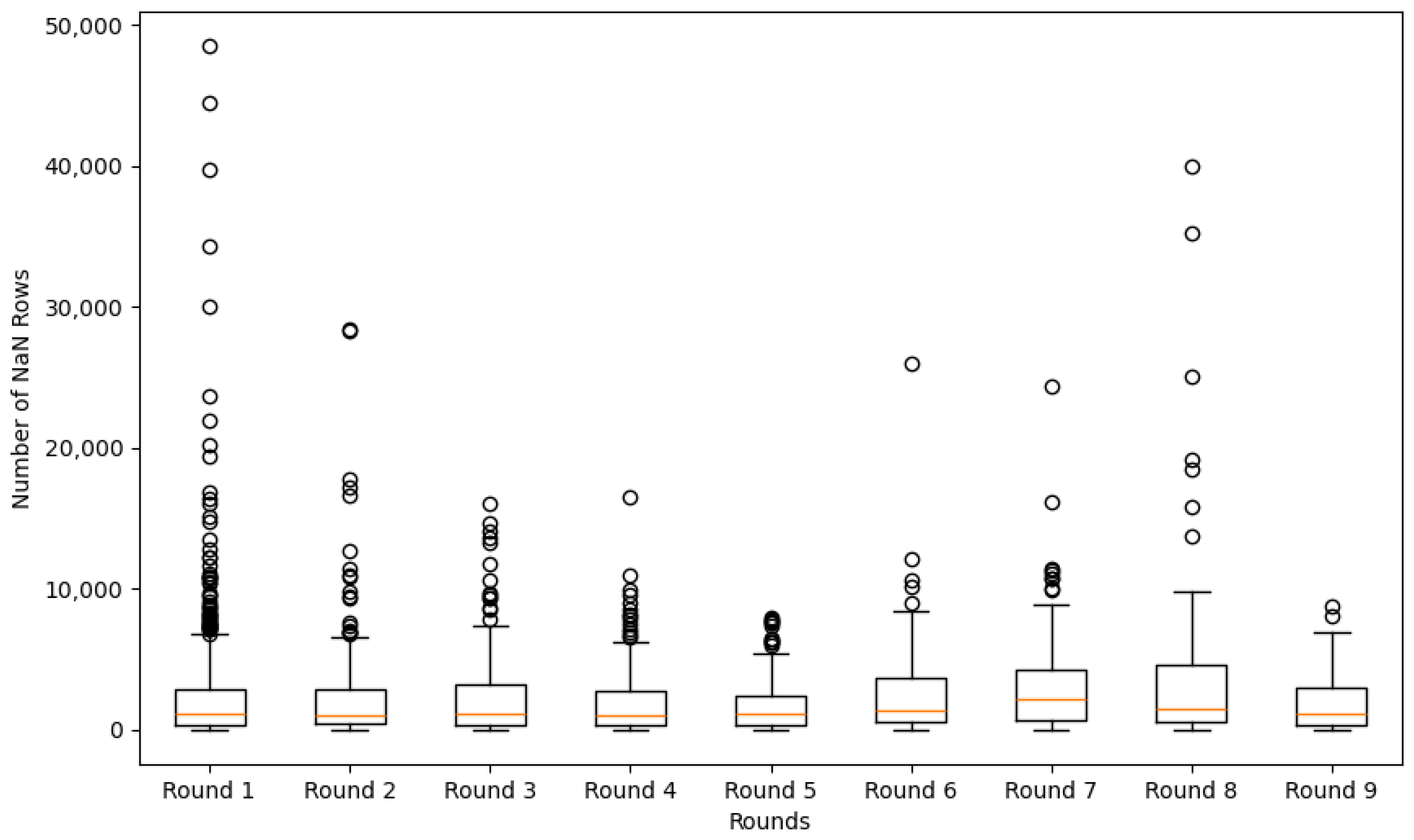
Mti 09 00042 g002
Figure 3. Box plot of missing (NaN) rows per CSV file across rounds, indicating data quality and sparsity distribution.
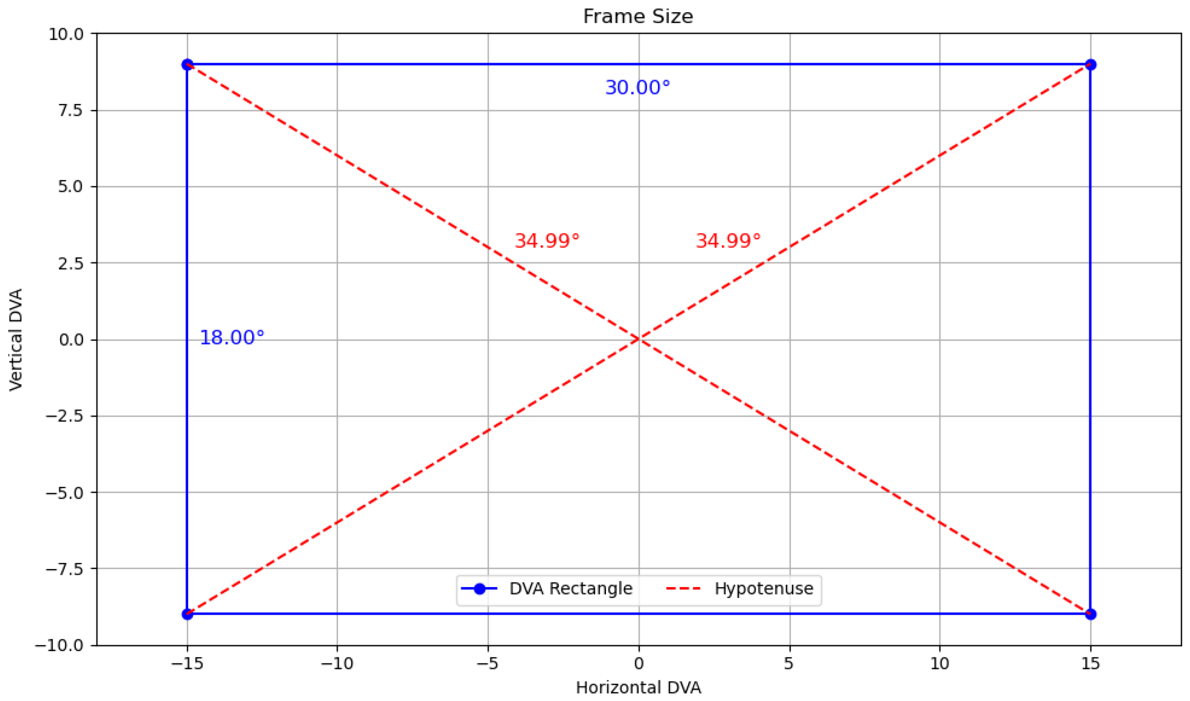
Mti 09 00042 g003
Figure 4. Visualisation of the screen frame used in the Random Saccade task, bounded within ±15° horizontal and ±9° vertical DVA.
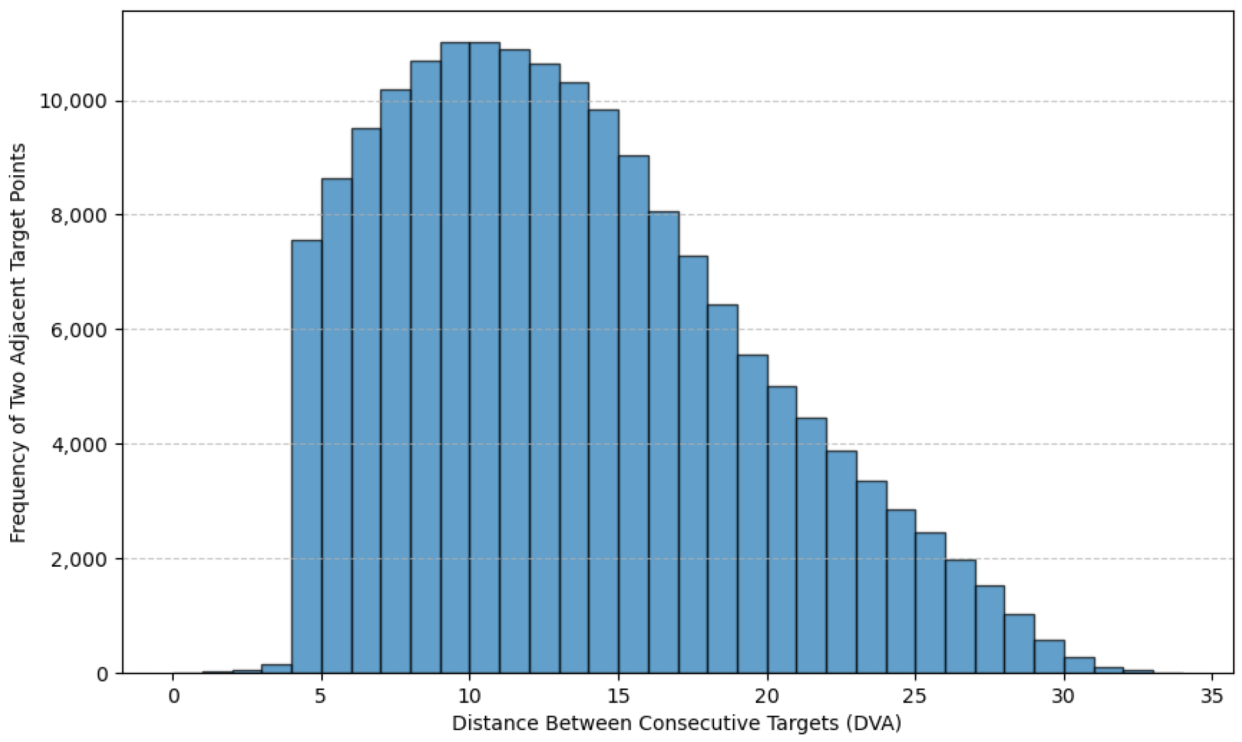
Mti 09 00042 g004
Figure 5. Distribution of spherical distances between adjacent target points, confirming task constraints of >2 dva displacement.
Mti 09 00042 g005
Figure 6. Classification of gaze points as inside or outside the defined display frame, based on target coordinate bounds.
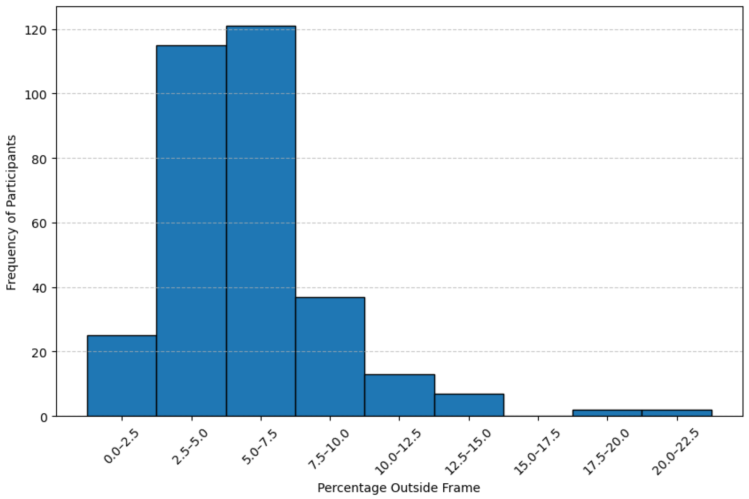
Mti 09 00042 g006
Figure 7. Distribution of the percentage of gaze points falling outside the frame across all participants.
Mti 09 00042 g007
Figure 8. NaN distribution among participants, categorised by the percentage of missing gaze points in each recording session.
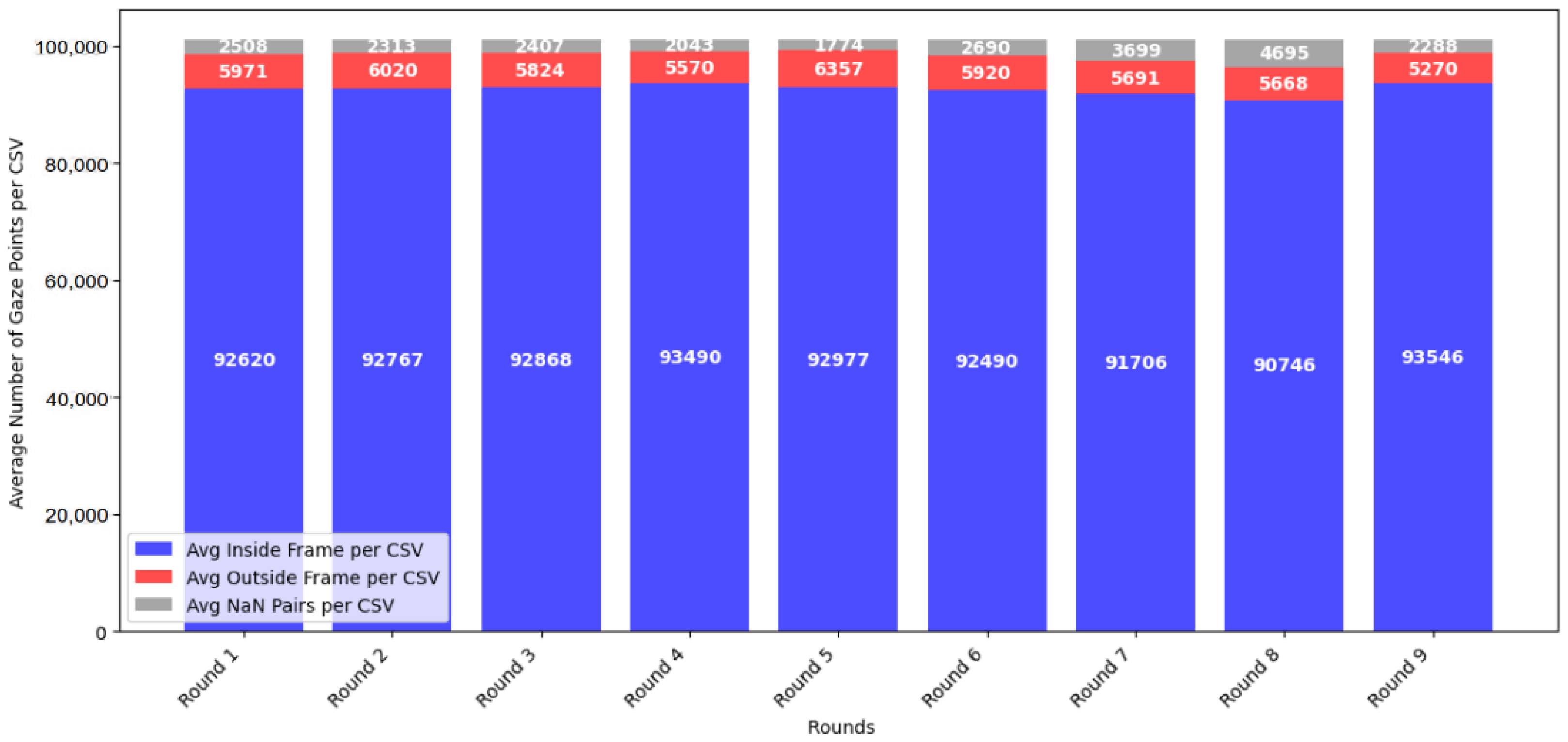
Mti 09 00042 g008
Figure 9. Average distribution of inside-frame, outside-frame, and NaN gaze points across all participant sessions.
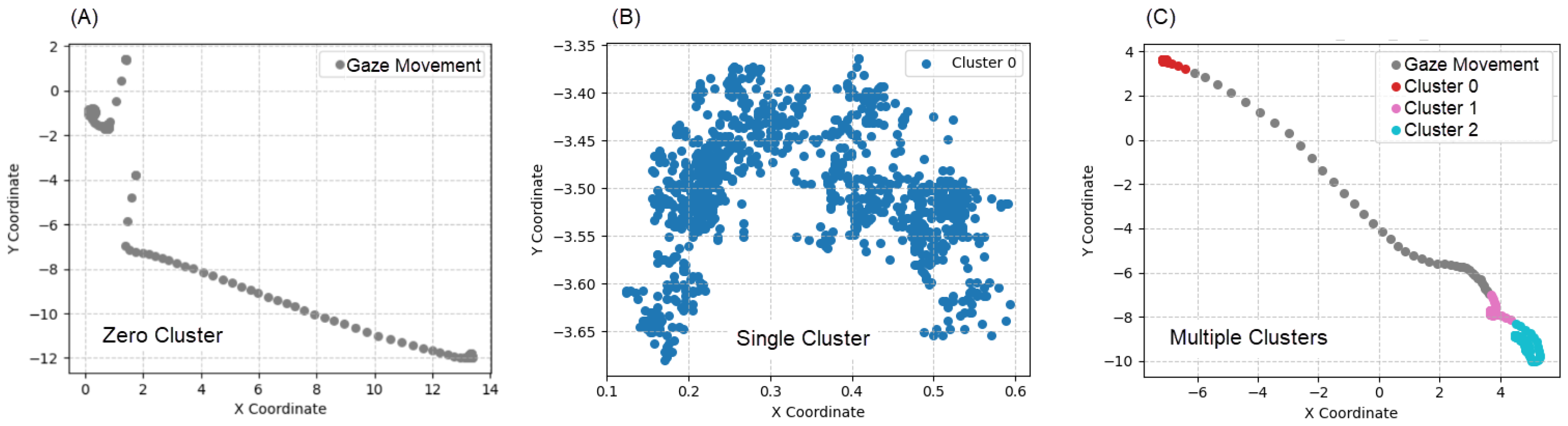
Mti 09 00042 g009
Figure 10. Cluster examples by count type: (A) Zero Cluster. (B) Single Cluster. (C) Multiple Clusters.
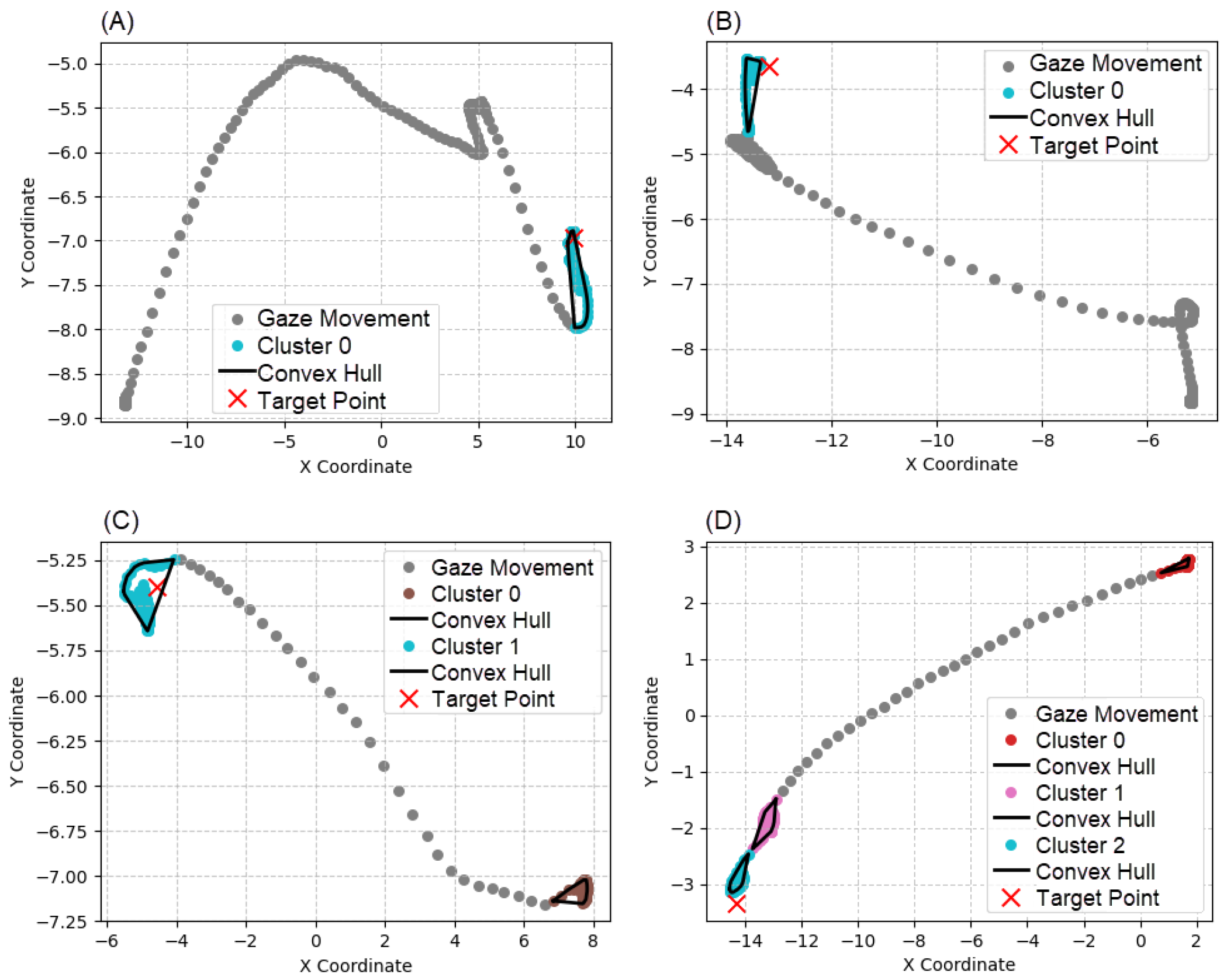
Mti 09 00042 g010
Figure 11. Examples of target point presence relative to clusters: (A) Single cluster, target inside. (B) Single cluster, target outside. (C) Multiple clusters, target inside. (D) Multiple clusters, target outside.
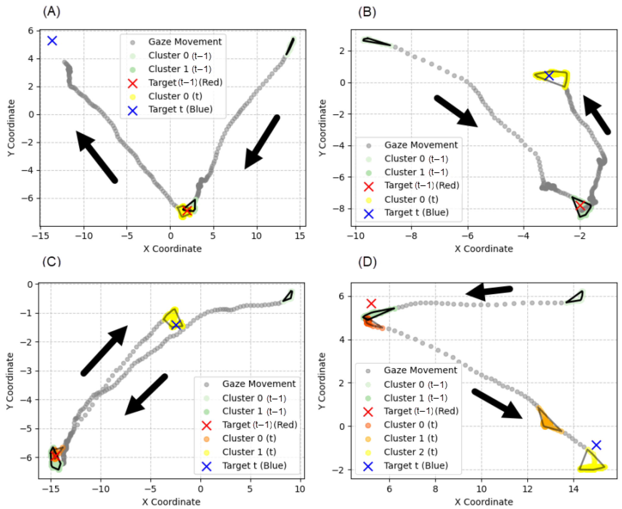
Mti 09 00042 g011
Figure 12. Examples of temporal relationships between clusters and targets: (A) Delayed single cluster. (B) Not-delayed single cluster. (C) Delayed multiple clusters. (D) Not-delayed multiple clusters. The arrows represent the direction of gaze movement.
Mti 09 00042 g012
Figure 13. Object extraction accuracy using k-NN under different window sizes and k values.
Mti 09 00042 g013
Figure 14. Accuracy comparison using k-NN with varying k values on the gaze dataset.
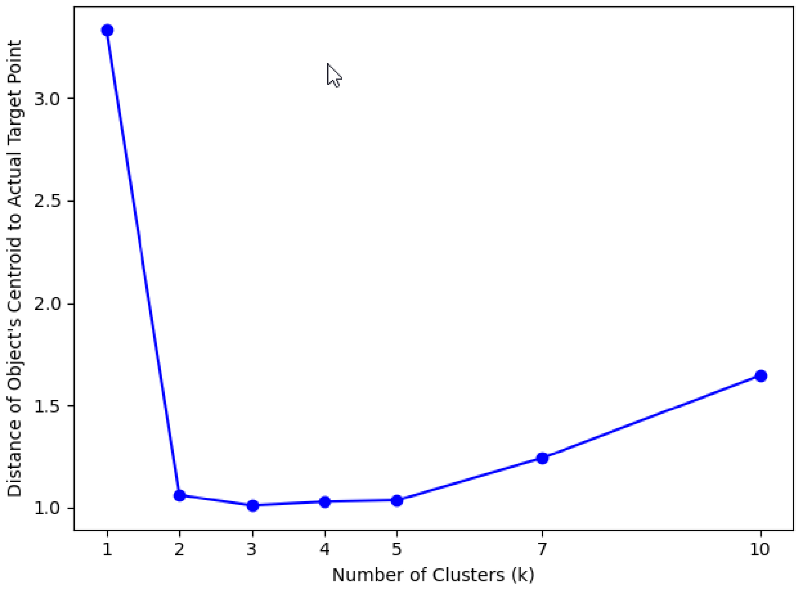
Mti 09 00042 g014
Figure 15. Accuracy comparison using k-Means clustering with different k values.
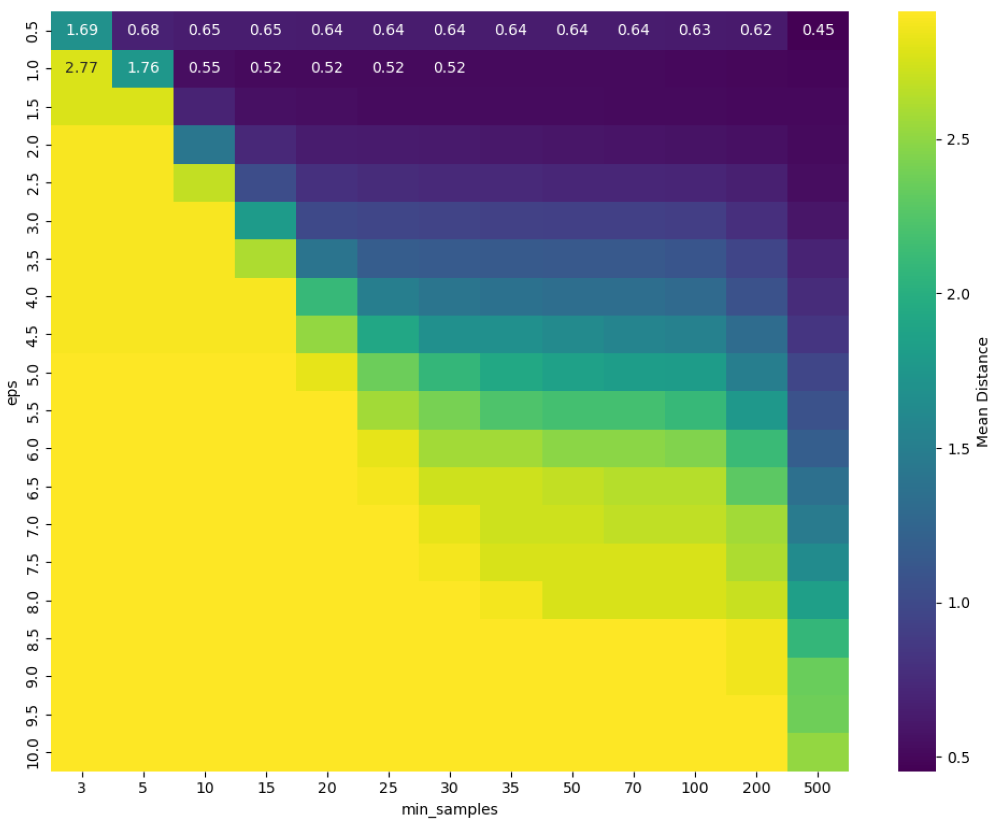
Mti 09 00042 g015
Figure 16. DBSCAN hyperparameter tuning for object extraction performance.
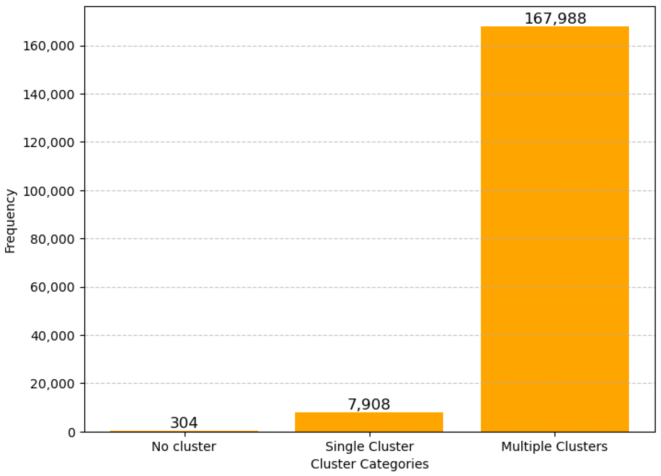
Mti 09 00042 g016
Figure 17. Frequency distribution of cluster count classifications across the dataset.
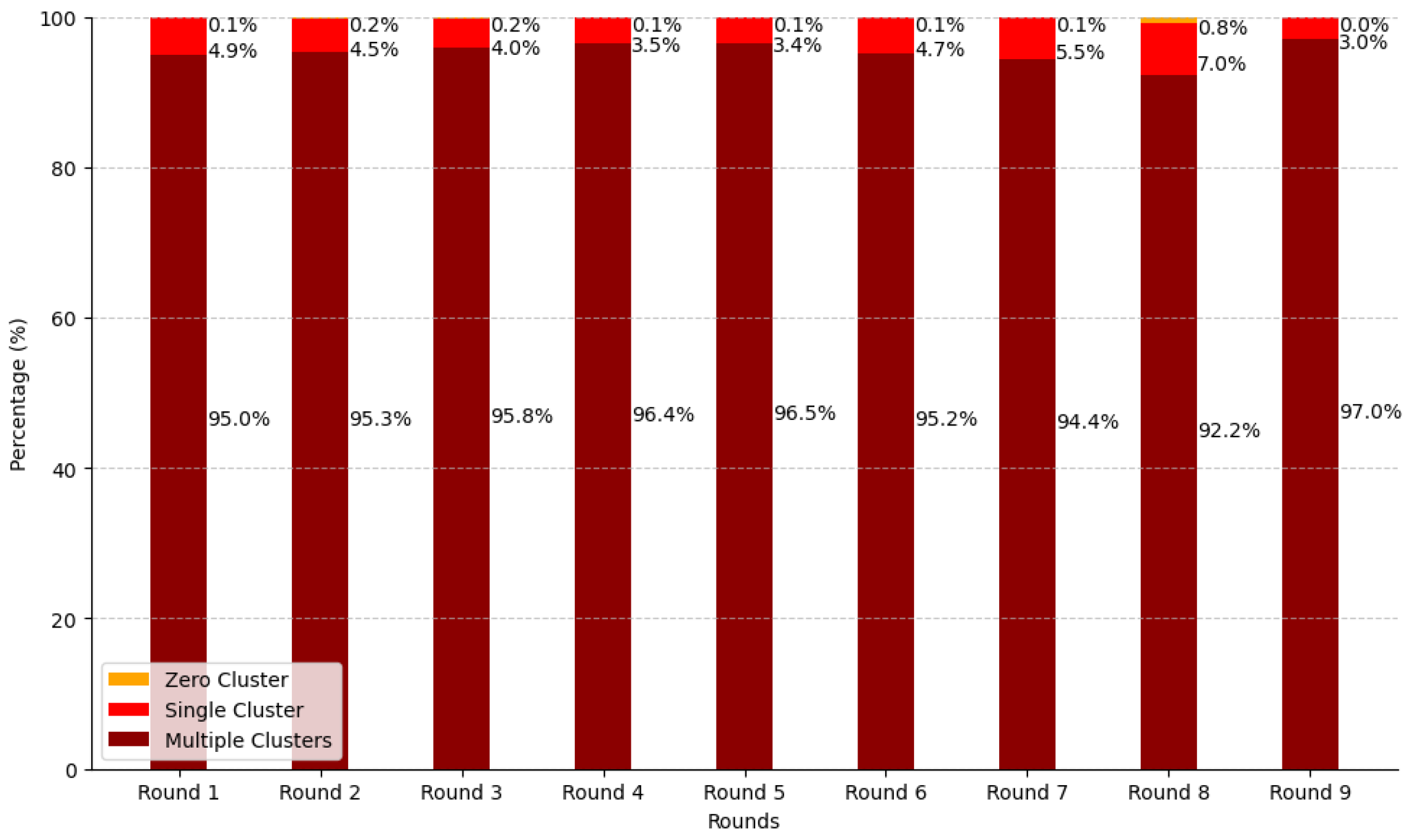
Mti 09 00042 g017
Figure 18. Stacked percentage distribution of cluster counts across different recording rounds.
Mti 09 00042 g018
Figure 19. 
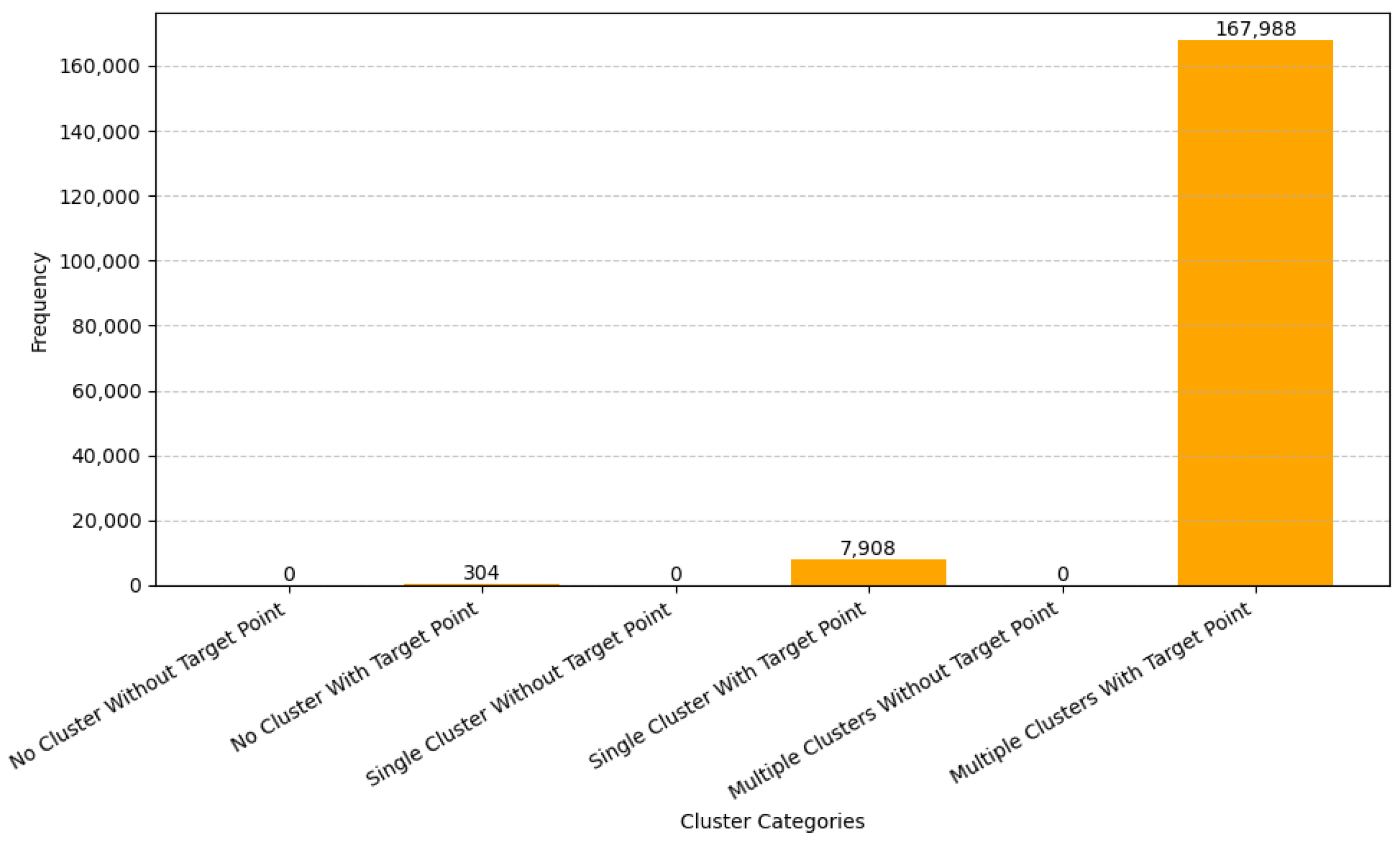
Distribution of clusters by presence or absence of the target point within them.
Mti 09 00042 g019
Figure 20. 
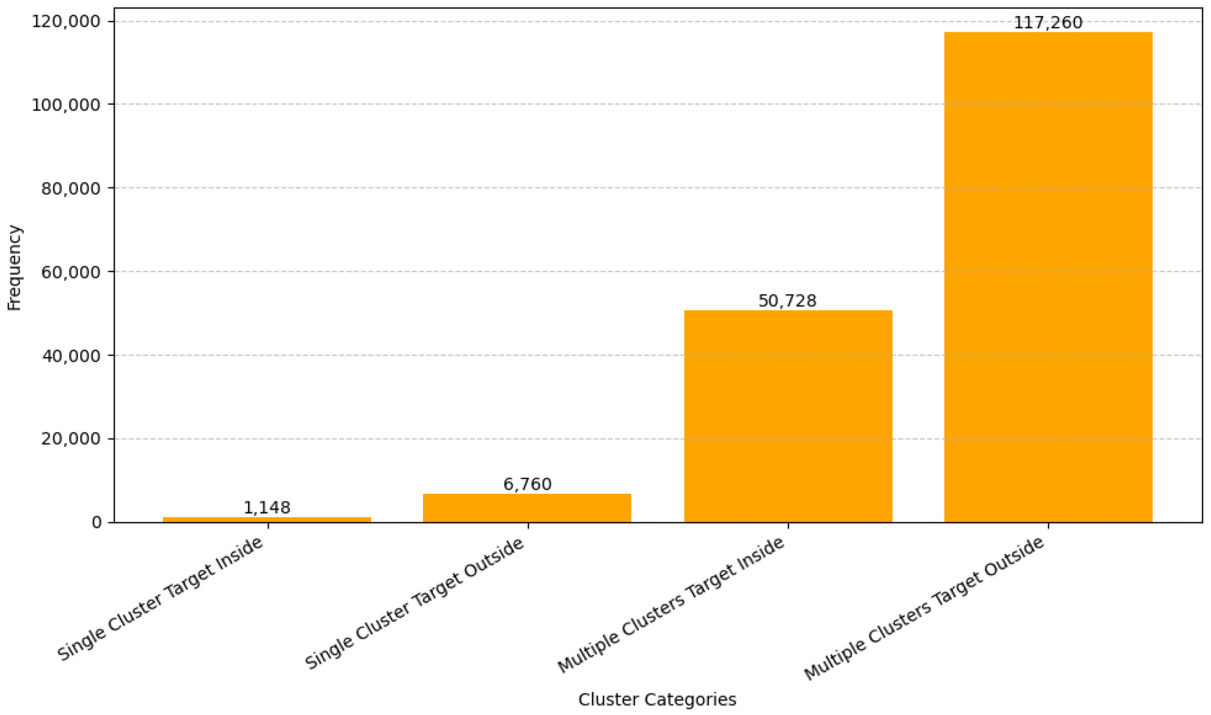
Distribution of combined cluster and target presence relationships (e.g., inside/outside).
Mti 09 00042 g020
Figure 21. 
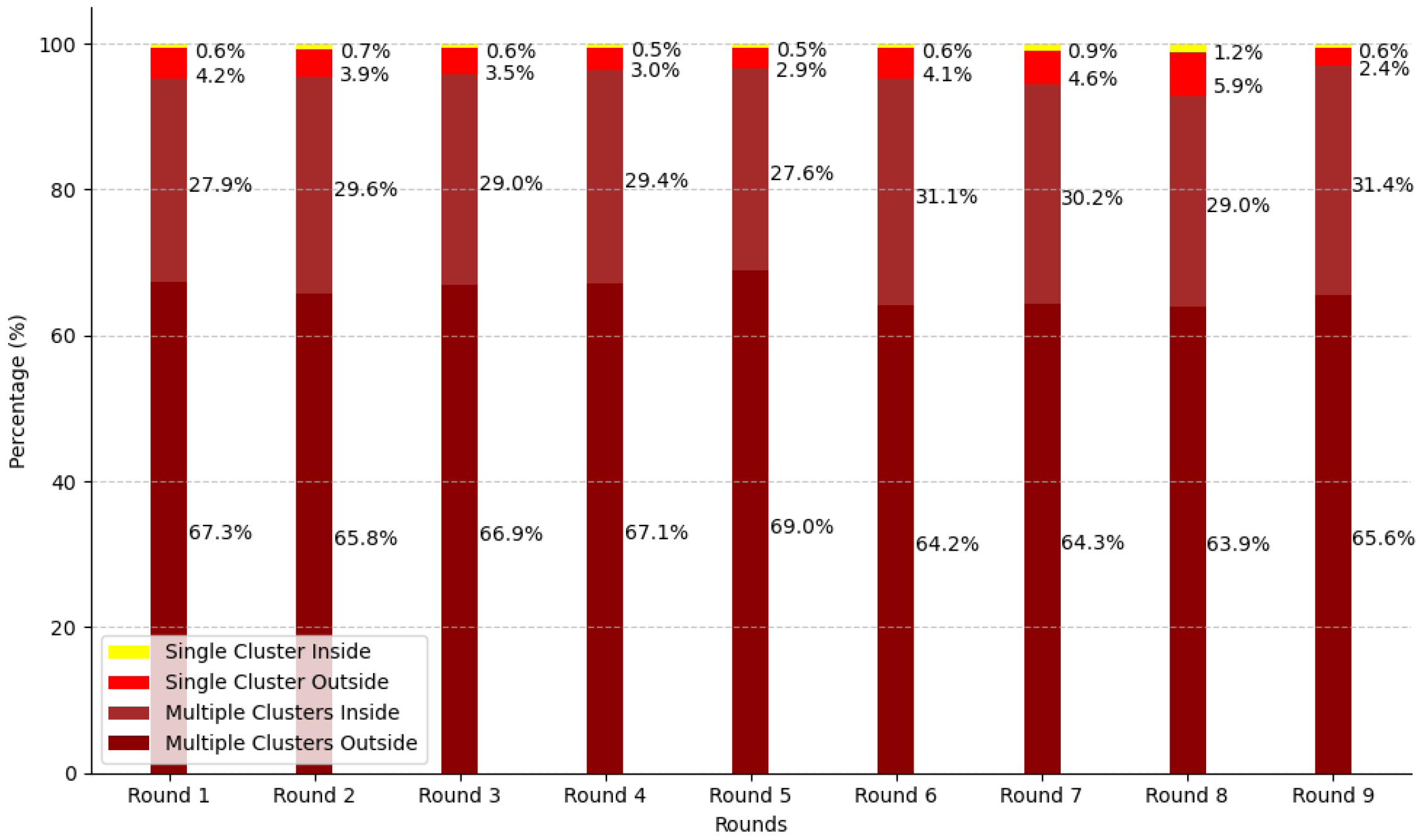
Stacked cluster distribution across rounds in percentage. The chart shows the proportion of different cluster categories per round.
Mti 09 00042 g021
Figure 22. Distribution of delayed and not-delayed cluster–target relationships.
Mti 09 00042 g022
Figure 23. 
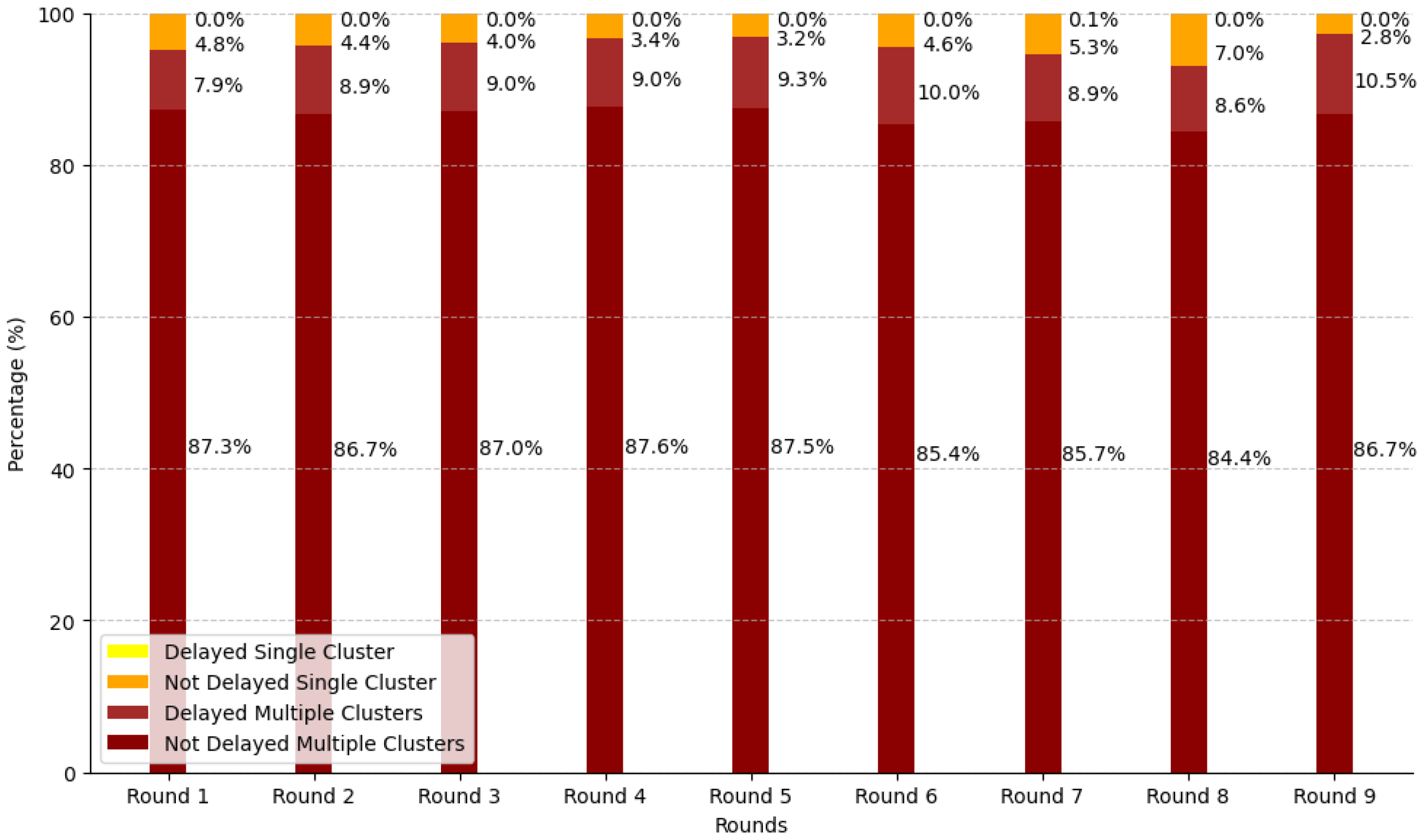
Percentage distribution of temporal cluster–target relationships across rounds.
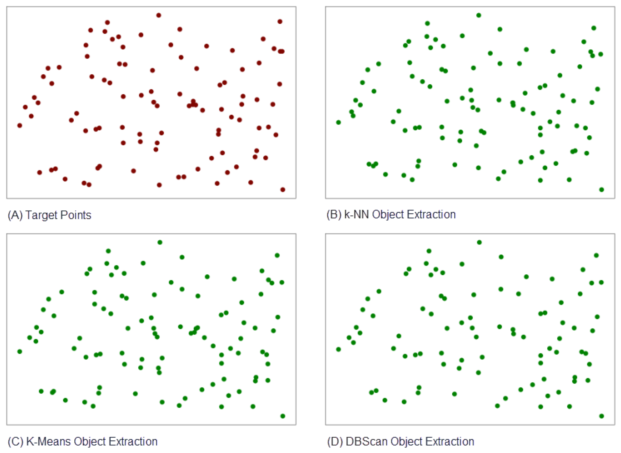
Mti 09 00042 g023
Figure 24. Example of Comparison Target Points and other object extraction methodologies result. (A) Target Points as ground truth for (B) k-NN Object Extraction, (C) K-Means Object Extraction, and (D) DBScan Object Extraction.
Mti 09 00042 g024
Table 1. Overview of clustering methods applied to gaze data across prior studies. Includes participant count, task type, clustering technique, and key findings.
StudyParticipantsYearTaskClustering MethodMain Findings
Nyström et al. [28]102010Event DetectionAdaptive Thresholds, Data-driven FilteringEmphasised filtering raw gaze data to accurately produce velocity and acceleration profiles, indirectly influencing clustering outcomes.
Kumar et al. [29]402019Reading (Metro Maps)Hierarchical ClusteringUtilised clustering to identify gaze behaviour groups, aiding interpretation of fixation and saccade metrics and facilitating visual exploration of reading patterns.
Hsiao et al. [30]612021Visual StimuliCo-clustering, EMHMMIdentified consistent eye-movement patterns across varying stimulus layouts by estimating individual Hidden Markov Models (HMMS) and applying co-clustering.
Table 2. Summary of exploratory data attributes across dataset rounds, including number of rows, NaN percentages, and gaze-point distributions.
RoundFilesParticipants100-Gaze Pairs GroupTarget PointsTotal ( x , y ) Pairs (in Million)% NaN Pairs% Inside Frame Pairs% Outside Frame
164432264,40064,40065.1 M2.4891.615.91
227213627,20027,20027.4 M2.2991.765.95
321010521,00021,00021.2 M2.3891.865.76
420210120,20020,20020.4 M2.0292.475.51
51567815,60015,60015.7 M1.7691.966.29
61185911,80011,80011.9 M2.6691.485.86
77035700070007.0 M3.6690.715.63
86231620062006.2 M4.6489.755.61
92814280028002.8 M2.2692.525.21
Table 3. Summary of Target Point Statistics. The variables x T and y T refer to the horizontal and vertical coordinates of the predefined target point shown during the Random Saccade task.
MetricMin ValueMax ValueStated MinStated MaxDifference MinDifference Max
x T −14.70256115.305838−15150.297439−0.305838
y T −9.3676478.604543−99−0.3676470.395457
Table 4. Adjacent target displacement statistics in degrees of visual angle (DVA), representing average spatial movement between successive target points.
RoundAverage Distance (DVA, Spherical)Minimum Distance (DVA, Spherical)Maximum Distance (DVA, Spherical)
Round 113.4664670.38288433.444873
Round 213.4840461.09297832.346398
Round 313.5061720.31814433.653568
Round 413.4606692.12619733.475838
Round 513.4292771.03615732.816737
Round 613.5167430.26340332.397405
Round 713.4611730.76583132.358234
Round 813.5201440.58259731.629944
Round 913.2084483.43466931.539671
Table 5. Statistics of gaze point values, showing minimum and maximum data distribution across the entire dataset.
MetricMin ValueMax Value
x−52.24181951.263111
y−41.15393136.633323
Table 6. Average object extraction accuracy across different clustering methods. Accuracy is calculated based on centroid-to-target distances.
Object Extraction MethodAverage Distance Accuracy Compared to Target Points
K-NN90.51%
K-means90.61%
DBscan90.87%
Table 7. Summary comparison of clustering methods (k-NN, k-Means, DBSCAN) based on the types of cluster classifications produced.
Cluster Typek-NN (k = 5)k-Means (k = 3)DBScan ( ε = 0.5, Min_samples = 500)
Cluster Count (CC)
No clusterNoNoNo
Single clusterYesYesYes
Multiple clustersNeed VoteNeed VoteNeed Vote
Cluster–Target Presence (C–TP)
No cluster with target pointNoNoNo
No cluster without target pointNoNoNo
Single cluster with target pointYesYesYes
Single cluster without target pointNo DataNo DataNo Data
Multiple clusters with target pointNeed VoteNeed VoteNeed Vote
Multiple clusters without target pointNo DataNo DataNo Data
Cluster–Target Relationship (C–TR)
Single cluster, target insideYesYesYes
Single cluster, target outsideNoNoNo
Multiple clusters, target insideNeed VoteNeed VoteNeed Vote
Multiple clusters, target outsideNoNoNo
Temporal Cluster–Target Relationship (TC–TR)
Delayed single clusterYesYesYes
Not-delayed single clusterNoNoNo
Delayed multiple clustersNeed VoteNeed VoteNeed Vote
Not-delayed multiple clustersNoNoNo
Table 8. Benchmark comparison between the proposed GCT and prior works. Summarises task types, metrics, and applicability to gaze analysis. The “N/A” values in the table represent instances where neither of the prior works reported standard classification metrics such as accuracy, precision, recall, or F1-score.
MethodTask/DatasetAccuracyPrecisionRecallF1-ScoreNotes
GCT (k-NN, k-Means, DBSCAN)Random Saccade (GazeBase)90.5–90.9%∼93–95%∼93–95%∼93–95%Supervised centroid-to-target classification; validated on 176,200 samples
Kumar et al. [29]Static map readingN/AN/AN/AN/AHierarchical clustering; no classification metrics reported
Hsiao et al. [30]Scene perception (natural images)N/AN/AN/AN/AEMHMM + co-clustering; evaluated using log-likelihood, not accuracy
Disclaimer/Publisher’s Note: The statements, opinions and data contained in all publications are solely those of the individual author(s) and contributor(s) and not of MDPI and/or the editor(s). MDPI and/or the editor(s) disclaim responsibility for any injury to people or property resulting from any ideas, methods, instructions or products referred to in the content.

