Article

An Efficient Testing Scheme for Power-Balanceability of Power System Including Controllable and Fluctuating Power Devices

Graduate School of Advanced Science and Technology, Japan Advanced Institute of Science and Technology, 1-1 Asahidai, Nomi City, Ishikawa 923-1296, Japan
*
Author to whom correspondence should be addressed.
Designs 2020, 4(4), 48; https://doi.org/10.3390/designs4040048
Submission received: 28 October 2020 / Revised: 20 November 2020 / Accepted: 20 November 2020 / Published: 25 November 2020
(This article belongs to the Special Issue Planning for Home Renewable Energy Systems)

Abstract

:
Renewable power sources are environmentally friendly power generation systems, such as wind turbines or photovoltaics; however, the output power fluctuations due to the intermittence and variability of these power systems can greatly affect the quality and stability of the power system network. Furthermore, the power fluctuations that are triggered by power load devices also have similar results on the power system. Therefore, it is essential to introduce power level control for controllable power devices and connection in order to lessen the effects of dynamic power fluctuations that are caused by fluctuating power source devices and load devices. The issue of power balancing as a part of power level control presented in this paper assigns power levels to controllable power devices and connections between power source devices and load devices to absorb dynamic power fluctuations. In this paper, we focus on power conservation law instead of detailed voltage or current-based network characterization and present a new power balanceability test for a power flow system that comprises of both fluctuating and controllable power devices. Our proposed power balanceability test can assure the existence of a power flow assignment of power devices and connections for any value of power generation and/or the consumption of fluctuating power devices. Our proposed power balanceability test method can be expressed as a linear programming problem, and it can be resolved in polynomial time complexity.

1. Introduction

The exhaustion of fossil fuels, a dynamic rise in power demand, together with gas emissions has encouraged the usage of renewable energy sources (RESs). Renewable energy sources e.g., wind and photovoltaic generation systems are an environmentally friendly alternative to the traditional power generation systems [1,2]. Nevertheless, the power generation from such power sources changes significantly or fluctuates due to their intermittent nature and weather conditions, which results in output power fluctuation that is not controllable [3]. Similarly, the power consumption of loads also changes dynamically due to the change in power device performance mode, power user preferences, etc. This power consumption is continuously growing due to the installation of smart power load devices that are deployed along with control and communication abilities [4,5,6,7]. Additionally, the development of electric cars and heat pumps is also adding to the peak of power demand. The combination of renewable-based power sources and continuously increasing power demand that is attached to the national grid have increased the risks of power quality and stability of the national grid.
The integration of distributed power sources and numerous smart loads leads to advanced power systems that are realized while using advanced research revolutions of smart power systems, distributed generation systems, power monitoring, and control, smart micro-grids, etc. [8,9]. The conventional power grids are huge, shared centralized power supply units. The new development towards small-scale power generation systems is promoted, which shows that the power supplying sources are positioned very close to power consumers. That is, the large power generation systems are substituted with small-scale power generation systems. Consequently, there is a great need for new approaches and sophisticated systems that can handle dynamic power generation patterns along with changing power consumption patterns.
The research developments that are related to demand-side management have also been recently highlighted because of the increase in power demand of residential and commercial sectors [10,11,12,13,14]. The power supply and demand of these sectors are changing rapidly due to the addition of small scale distributed power generating resources, like storage batteries, photovoltaic, wind turbines, and fuel cells [15,16,17]. Some examples of such residential and commercial sectors with multiple power sources and numerous power consumers are Nano-grid, Community-grid, Micro-grids including smart homes and offices [18,19,20,21]. That is, such power management systems need to have a sophisticated power flow control method that can manage power flows coming from multiple power sources including renewables and dynamic power demands including numerous smart power-consuming devices.
The uncontrollability of power generation of fluctuating power sources (i.e., renewable power sources) and power consumption of fluctuating power loads is a challenging task for power balancing of the power system [22,23]. In order to achieve power balance, support from controllable source devices and power load devices appears to be an encouraging technology [24,25,26]. Additionally, advanced power technology equipped with sensing and controlling capabilities, e.g., smart sensors and actuators, power provisioning controllers, can play an important role in real-time power sensing, transmission, and control. The high control-ability of these power devices along with the transmission of power data can help to control power levels accurately on each power flow connection.
Therefore, because the power levels of real physical power systems alter every time step, the problem of whether the given power system under consideration (i.e., our power flow control problem) has a feasible solution or not in individual time instance is an essential problem to solve. In our previous research work [27,28], we have discussed two types of solvability conditions, one for a given power flow system with given power generation and demand levels of the fluctuating power source and load devices to have a feasible solution Level 1 solvability, and the other for a given power flow system with arbitrary (but within given lower limit and upper limit) power level of fluctuating source and load devices to have a feasible solution Level 2 solvability.
In the past, power flow management methods with different objectives and techniques have been proposed [26,29,30,31]. In [32], a flexible multi-energy power generation system is introduced that consists of multiple power sources and numerous power-consuming devices. Every power source is connected with a group of power-consuming devices (not all power consuming devices) to manage long term uncertainty of power supply and demand. Another study in [33] shows the multi-energy microgrid that consists of multiple power sources, including renewable power sources, and it tries to manage long-term as well as short-term uncertainty of power sources. The ultimate goal of these papers is to improve the flexibility of power-consuming devices in order to efficiently accommodate the uncertainty of power sources. However, the power system design and the consideration of design guidelines to guarantee the power system robustness against power fluctuations of fluctuating source/load in real-time is not discussed, which is the main consideration of our research.
This particular paper presents a new robustness test mechanism for a power system that consists of controllable and uncontrollable/fluctuating power devices. This method can guarantee the existence of a feasible solution for any measured power level of fluctuating power devices, that is, a power flow system that satisfies Level 2 solvability. The test method can be expressed as a linear programming problem, which can be solved with polynomial time complexity. The time complexity improvement is the new contribution of this paper. Our previous paper used a method having the exponential order time complexity, whereas this particular paper proposes a new method having the polynomial order time complexity, which is quite different from the previous one, especially when the number of power devices increases.
This particular paper is designed, as Section 2 presents a power flow system and its overview with illustration, and the types of power source/load devices and power flow connections among power source devices and load devices. Section 3 defines the issue of solvability of our proposed power control problem. A new novel solvability condition for a power flow system for any value of the power of fluctuating power devices is explained in order to demonstrate the system property “robustness” of the power system under consideration, as in Section 4. The Linear Programming problem design, formulation, and realization are discussed with the help of demonstration in Section 5. Finally, the concluding remarks are discussed in Section 6.

2. System Overview

The power flow system in this paper comprises of distributed power source devices, numerous power load devices, and power flow connections that connect power devices. We consider two types of power devices; controllable, and uncontrollable. The controllable power devices can perform the task of supplying power or absorbing power in order to accommodate power fluctuations (i.e., excess or shortage in power) caused by fluctuating power generation/demand. These power devices also help to make the whole power system robust against the consequences of power fluctuations. This section explains the details of our power flow system model and our Power Flow Control Problem.

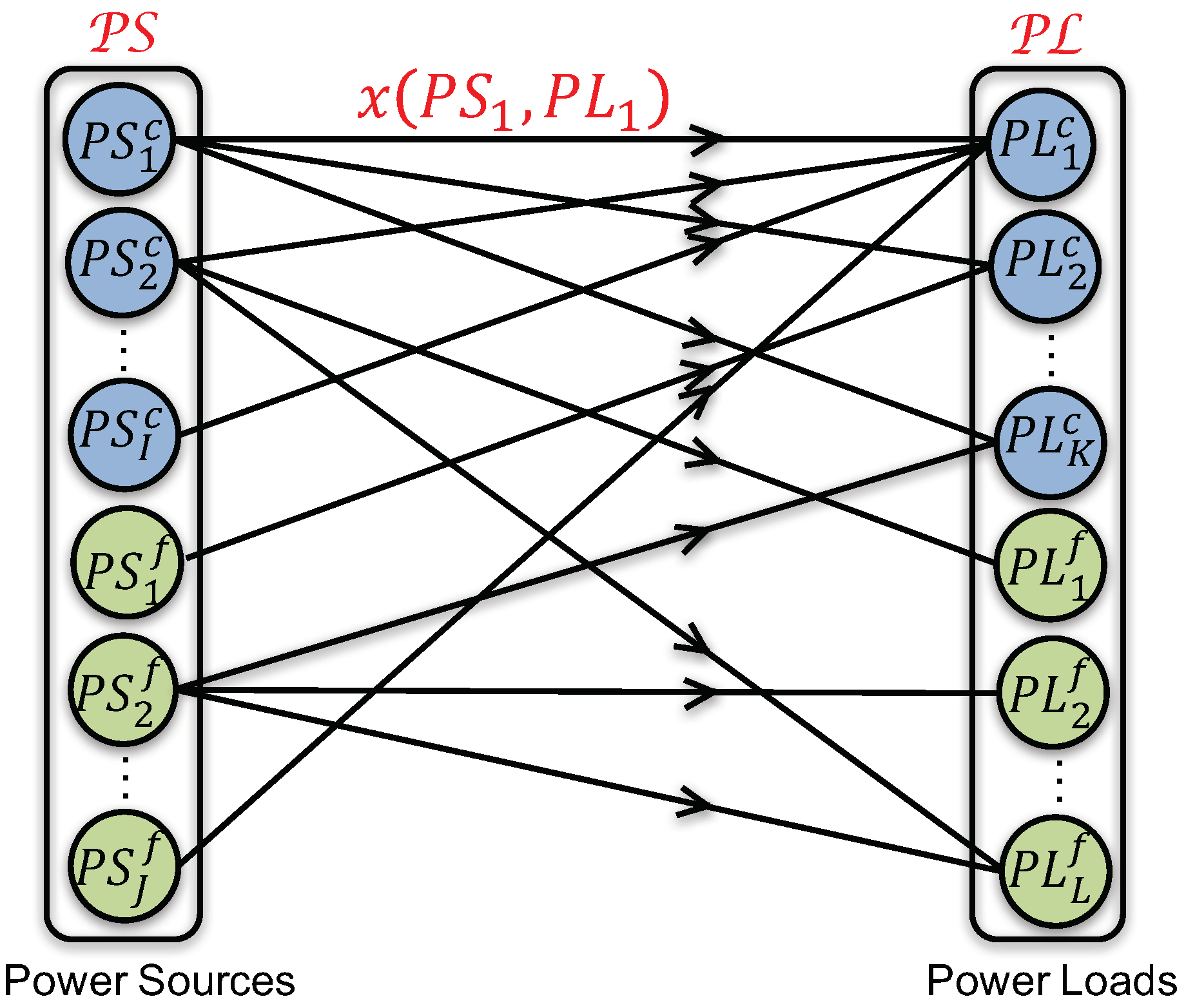
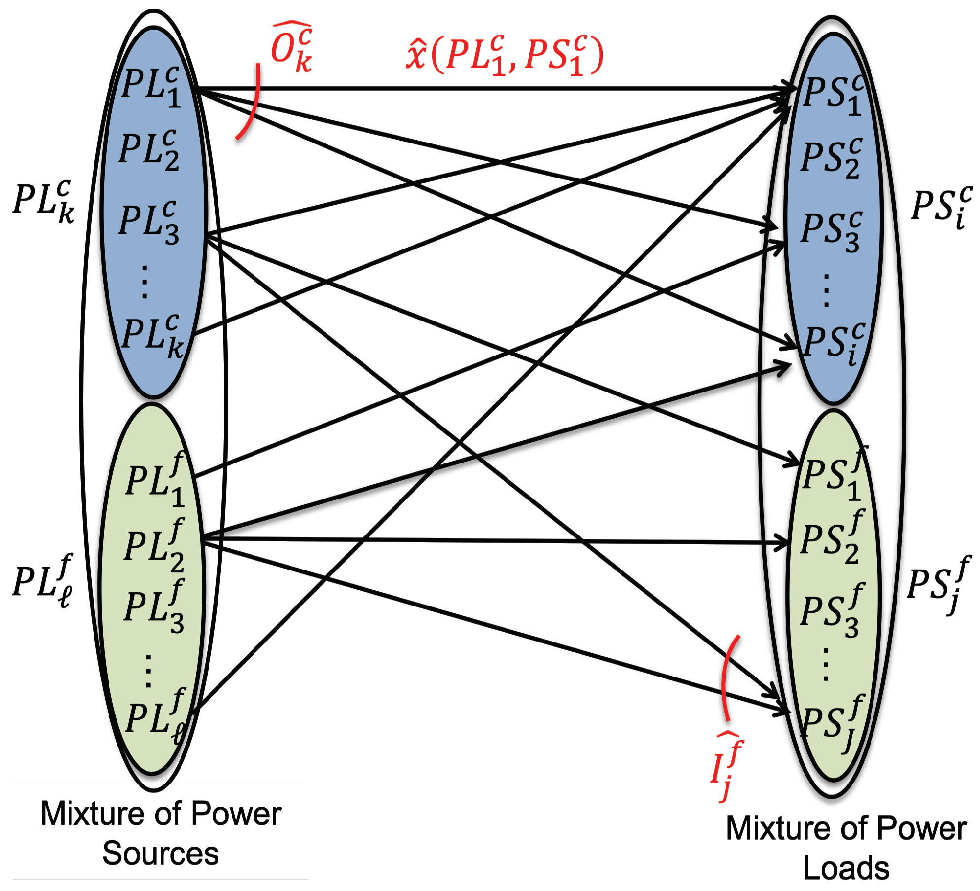
2.1. Illustration and Types of Power Devices

In this subsection, the representation of power devices, types of power devices, and connections between them are explained.
A power source device ( P S ) is an electric device that supplies power to power load device(s), e.g., wind turbine, utility grid, photo-voltaic, etc. A power consuming/load device ( P L ) can be defined as an electric power device that consumes electric power that is supplied by power source device(s). These power devices (i.e., source devices and load devices) are categorized into two types based on their features and functionality, and named as controllable and uncontrollable. In this paper, we will use word "fluctuating" for uncontrollable power sources and loads. The representation of these devices can be shown as P S c / P L c and P S f / P L f . A controllable power device P S c / P L c can control the power (generation/demand), while the fluctuating power device P S f / P L f cannot control its generation/demand. A controllable power source/load is equipped with a sensing and controlling unit in order to measure actual power levels, communicate with other power devices, and control its power according to the assigned power.
All of the power source devices with different types can be denoted as, PS = { P S 1 c , P S 2 c , , P S I c , P S 1 f , P S 2 f , , P S J f } = { P S 1 , P S 2 , P S 3 , , P S I + J } , where I and J represent the entire number of controllable and fluctuating power source devices, respectively. Likewise, all power load devices can be defined as, PL = { P L 1 c , P L 2 c , , P L K c , P L 1 f , P L 2 f , , P L L f } = { P L 1 , P L 2 , P L 3 , , P L K + L } , where K and L indexed the entire number of controllable and fluctuating power load devices.
The real physical power levels (i.e., supply and consumption) of source devices and load devices will be symbolized as p s i c , p s j f , p k c and p f , respectively, for P S i c , P S j f , P L k c , and P L f .
Every power device P S / P L is bounded with given minimum and maximum power restrictions that further demonstrate the operation mode and performance range of that power device. The minimum power level limitation p s i c m i n and maximum power level limitation p s i c m a x express the capability of a controllable power source device P S i c in supplying power to load devices. The actual power level p s i c that is generated by P S i c is bounded as,
p s i c m i n p s i c p s i c m a x
Additionally, the power bounds will be shown as p s j f m i n and p s j f m a x correspondingly, for P S j f and the power supply p s j f is assumed to be limited as,
p s j f m i n p s j f p s j f m a x
As for the power consumption level p k c of controllable power load device P L k c with minimum and maximum power level limitations p k c m i n and p k c m a x , and for consuming power p f of fluctuating load device P L f with power level limitations for minimum and maximum p f m i n and p f m a x are given as,
p k c m i n p k c p k c m a x
p f m i n p f p f m a x
On the other hand, a power flow connection is defined as a pair of a power supplying device P S and a consuming device P L , ( P S m , P L n ) , and the set X of connections is defined as X PS × PL . The arrangement of power devices in real physical world and power flow connections between power devices can be exhibited as a bipartite representation that is presented in Figure 1.
The system model shows incomplete power flow connections between power source devices and power load devices. That is, power devices with power flow connections show that the power is being supplied or transferred via connected connection, whereas no power flow connections with the power device show that the power cannot be supplied or transferred from that power device to other power devices.
Each power flow connection ( P S m , P L n ) is associated with some power level expressed in Watt x ( P S m , P L n ) in order to represent the amount of power sent from a power source device P S m to a power load device P L n through this power flow connection; this is a non-negative real number. In this paper, we only deal with an active power in Watt.
The conventional power flow is based on voltage, current, and phase; thus, the formulation is non-linear and non-convex in general. However, the power flow control problem thar is proposed in this paper has been formulated, as given in [34].

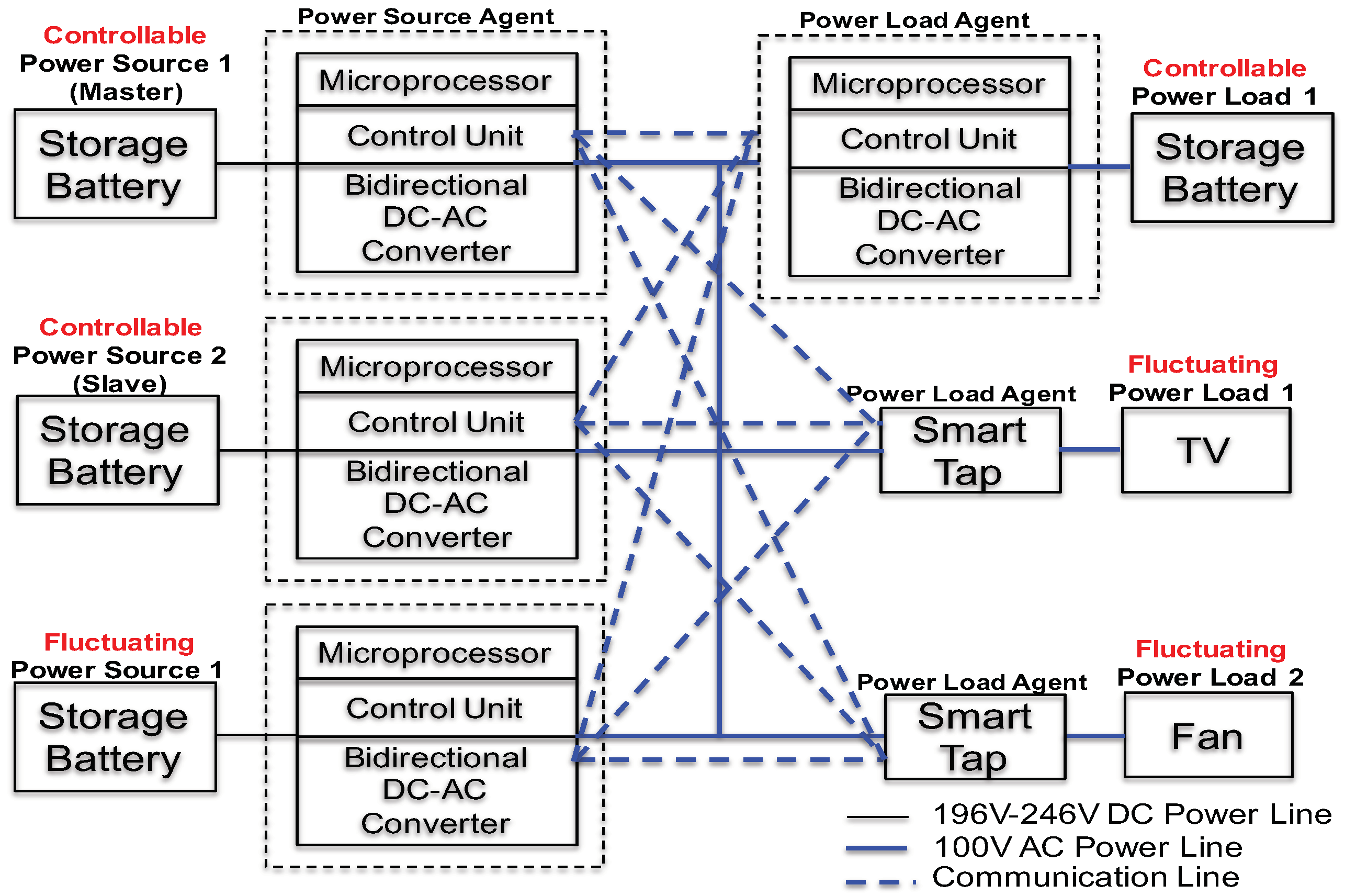
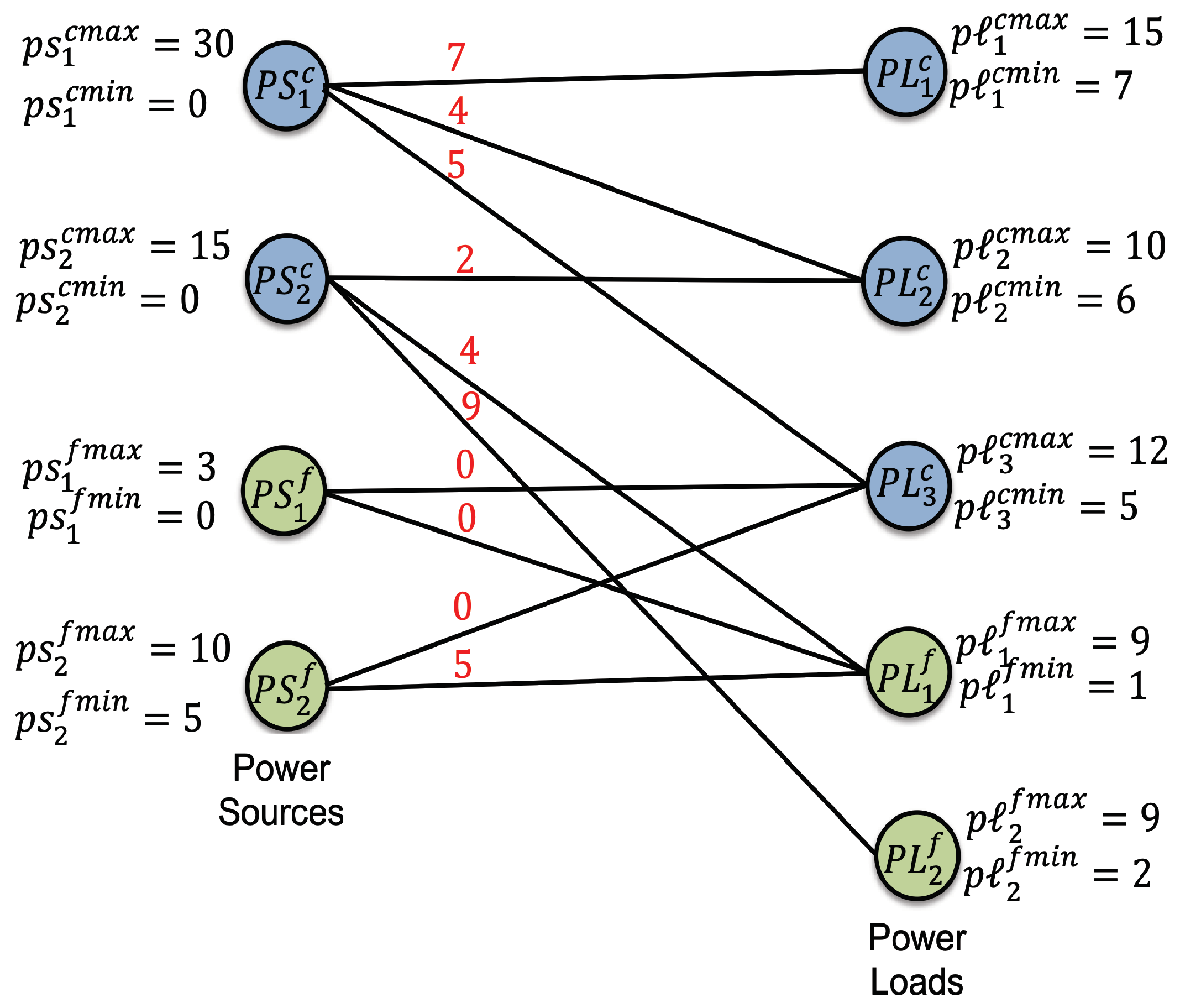
2.2. An Example of a System to Be Considered

The system model described in the previous subsection can be applied on a real physical system, as given in Figure 2 and Figure 3 with incomplete power flow connections.
In this physical setup, four storage batteries with smart power distributer [25], fluctuating power loads, i.e., television and a fan with smart power sensors, are linked via a shared power line as AC 100 V. One storage device is selected to be a controllable power source, P S 1 c , second storage device is acting as an emulator i.e., photovoltaic (PV) generating source ( P S 1 f ), third storage device is used as controllable power source (i.e., P S 2 c ), and the remaining storage battery is used as a controllable load (i.e., P L 1 c ). The PV generation emulator is responsible for generating user-defined values of power generation. These user-defined values show the dynamics of the physical PV generation system.

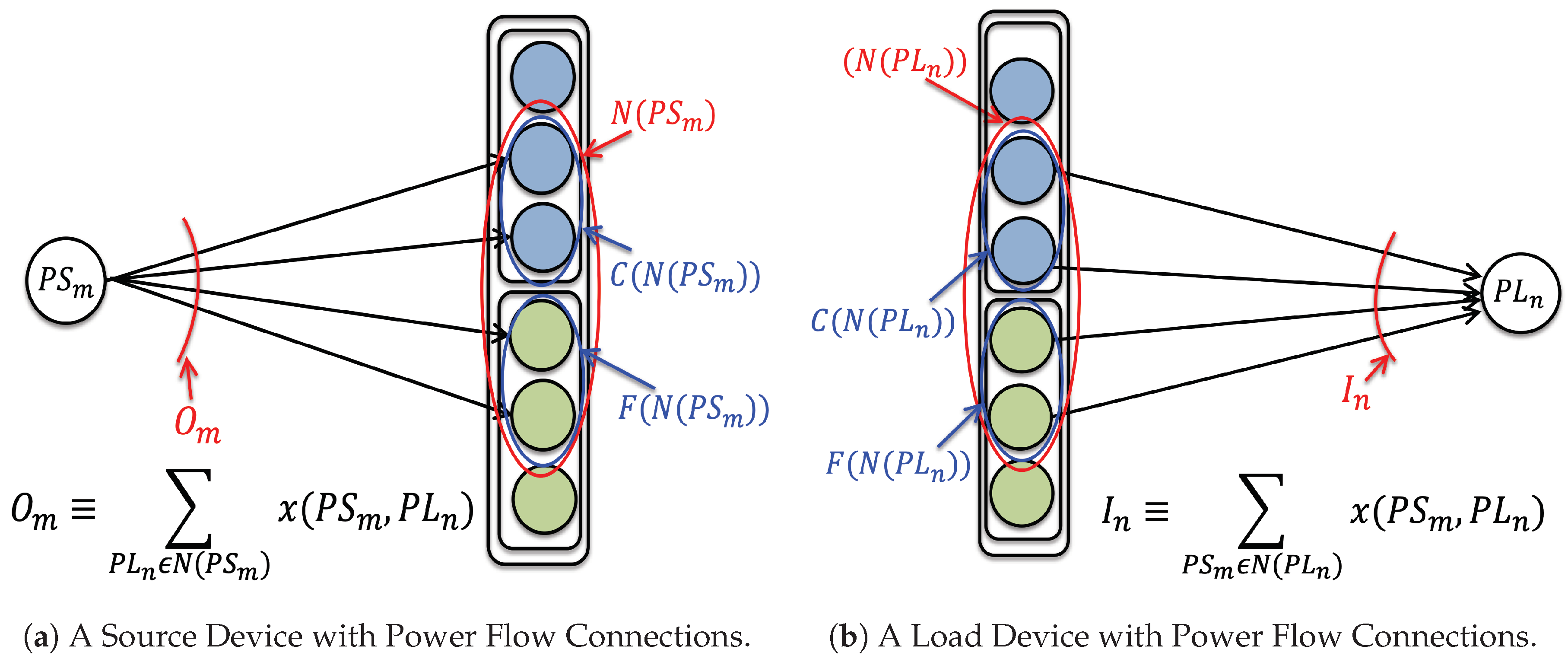
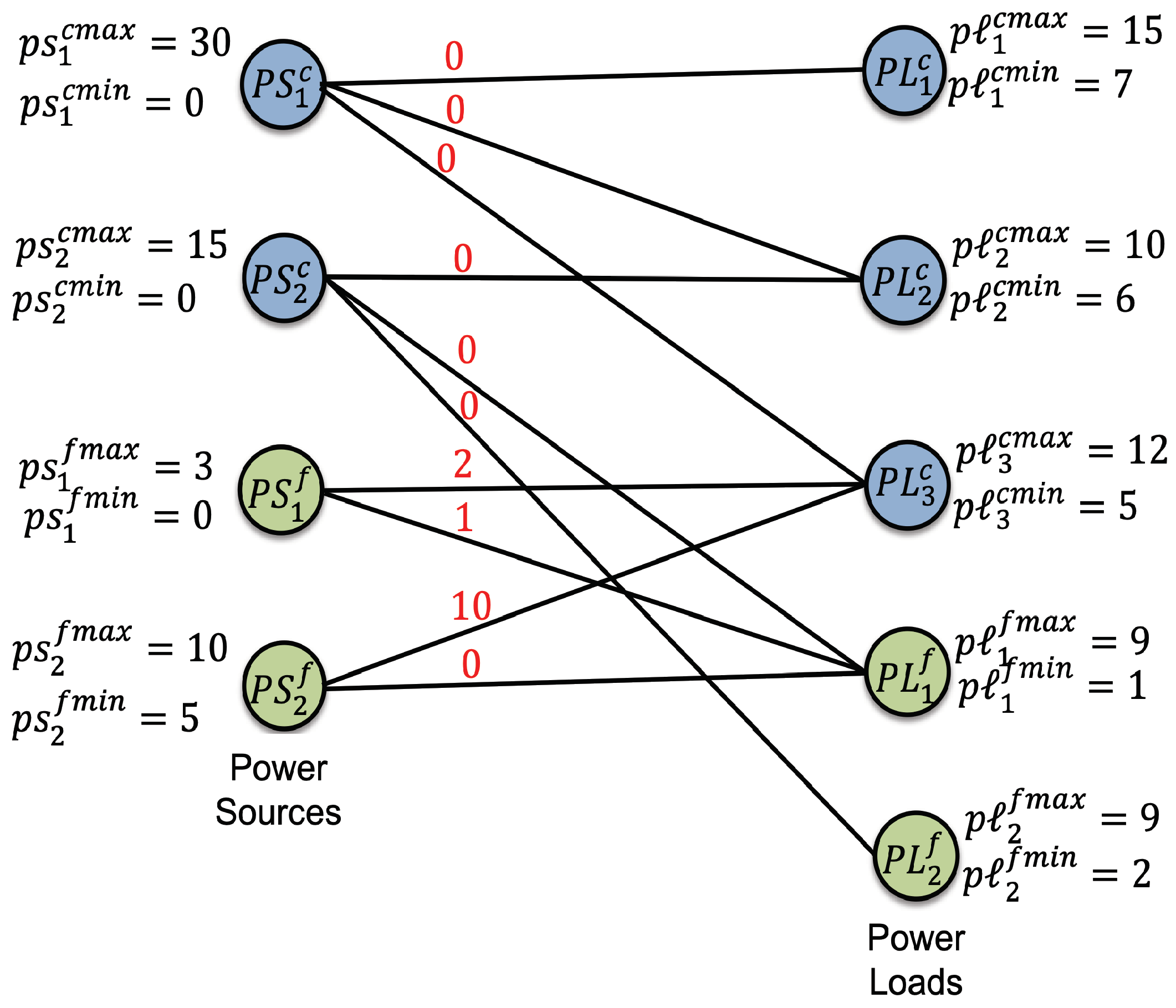
2.3. Power Flow Control

Because the measured power level of a fluctuating source/load alters a lot because of its characteristics and operation mode, the amount of power flow on each connected power flow connection must be altered. A power agent is attached to each device that is responsible for measuring the power levels of attached power device at each time step. In our paper, the word “fluctuation” is used for uncontrollable power levels for both generating and consuming powers no matter whether the fluctuations are small or big. Therefore, because the solvability conditions in our system deal with instantaneous power levels, any type of fluctuation that is caused by fluctuating power sources or loads is accommodated in our proposed system.
A power control algorithm is mandatory for a stable system in order to manage dynamic fluctuations of fluctuating source/load. The measured power information of fluctuating source/load by power agent is used to compute the power levels for controllable source/load devices and power flow connections while keeping the power balance constraint. This shows that the total power supply/generation by entire set of power source devices is completely used/consumed by power load devices, and the entire set of power load devices obtain enough power from connected power source devices.
Each power flow connection connects a source device P S to its connected or neighbors devices on the other side. The set of connected power devices of P S m is represented as N ( P S m ) ; these connected devices can be divided into controllable connected devices and fluctuating connected devices as C ( N ( P S m ) ) and F ( N ( P S m ) ) , respectively. For the illustration of connected devices and power flow connections, please see Figure 4a,b.
The summation of powers on all outgoing connections, O m , of source device P S m can be expressed as,
O m = Δ P L n N ( P S m ) x ( P S m , P L n )
Accordingly, the summation of powers on all incoming connections, I n , of a load device, P L n , can be shown as,
I n = Δ P S m N ( P L n ) x ( P S m , P L n )
For the power flow control and its solution, the total supplying power p s m of a power supplying device P S m must be equivalent to the all outgoing flow connections, O m as,
O m = p s m ,
The power demand p n of the power load device P L n must be equivalent to the total of all incoming power flow connections of this load device as,
I n = p n .
The overall target of our power flow control is to identify (i) the associated power levels as p s i c and p k c of controllable devices both sources and loads and (ii) power assignment for individual power flow connection x : X R + by using the received power levels from sensors p s j f and p f of fluctuating devices including source and load devices, so that (5) and (6) are fulfilled together along with power level constraints of power devices given as (1) and (3).

3. Problem Discussed in This Paper

This paper shows solvability issues of power flow control, which is, whether a given power system with power source devices, power load devices, and power flow connections has a feasible power flow assignment x, which satisfies Equations (5) and (6).
In our previous research work [27,28], we have discussed two types of solvability conditions, one for a given power flow system with given power generation and demand levels of fluctuating power source and load devices to have a feasible solution Level 1 solvability, and the other for a given power flow system with arbitrary (but within given lower limit and upper limit) power level of fluctuating source and load devices to have a feasible solution Level 2 solvability shown as condition 1-1 and condition 1-2. These conditions are presented as “Theorem-1” in this paper. Please refer to Appendix A to understand the meaning of Theorem 1.
The ultimate objective of this paper is to find a new revised solvability condition that improves the time complexity for the testing from the exponential order to the polynomial order.
Theorem 1.
The proposed control problem can find the feasible solution of a power flow system if and only if the given two solvability conditions are satisfied.
Condition 1-1:
S PS , P S i c C ( S ) p s i c m i n + P S j f F ( S ) p s j f m a x P L k c C ( N ( S ) ) p k c m a x + P L f F ( N ( S ) ) p f m i n
Condition 1-2:
T PL , P S i c C ( N ( T ) ) p s i c m a x + P S j f F ( N ( T ) ) p s j f m i n P L k c C ( T ) p k c m i n + P L f F ( T ) p f m a x
For more information, an example of S PS , N ( S ) and T PL , N ( T ) is illustrated in Figure 5 and Figure 6.
In order to guarantee the continuous operation of the power flow system consisting of both types of power devices with uncertainty of supplying and consuming power levels of fluctuating power devices, the power system needs to satisfy above stated conditions.
In order to apply the Theorem 1 to a power system, we need to generate all of the subsets of power source devices and load devices that causes time complexity in the exponential order with increasing number of power source devices and load devices. Hence, there is a need to find an alternative way to decide whether a given system always has a feasible power flow assignment or not with a decreased time complexity.
For this reason, a new “Theorem 2” is proposed in this paper. The proposed Theorem uses a Linear Programming (LP) solver in order to identify the power system while keeping (i) the physical constraints of power devices (i.e., physical constraints) (ii) and power flow connections between power source devices and power load devices in order to ensure the existence of solution by fulfilling the conditions 1-1 and 1-2.

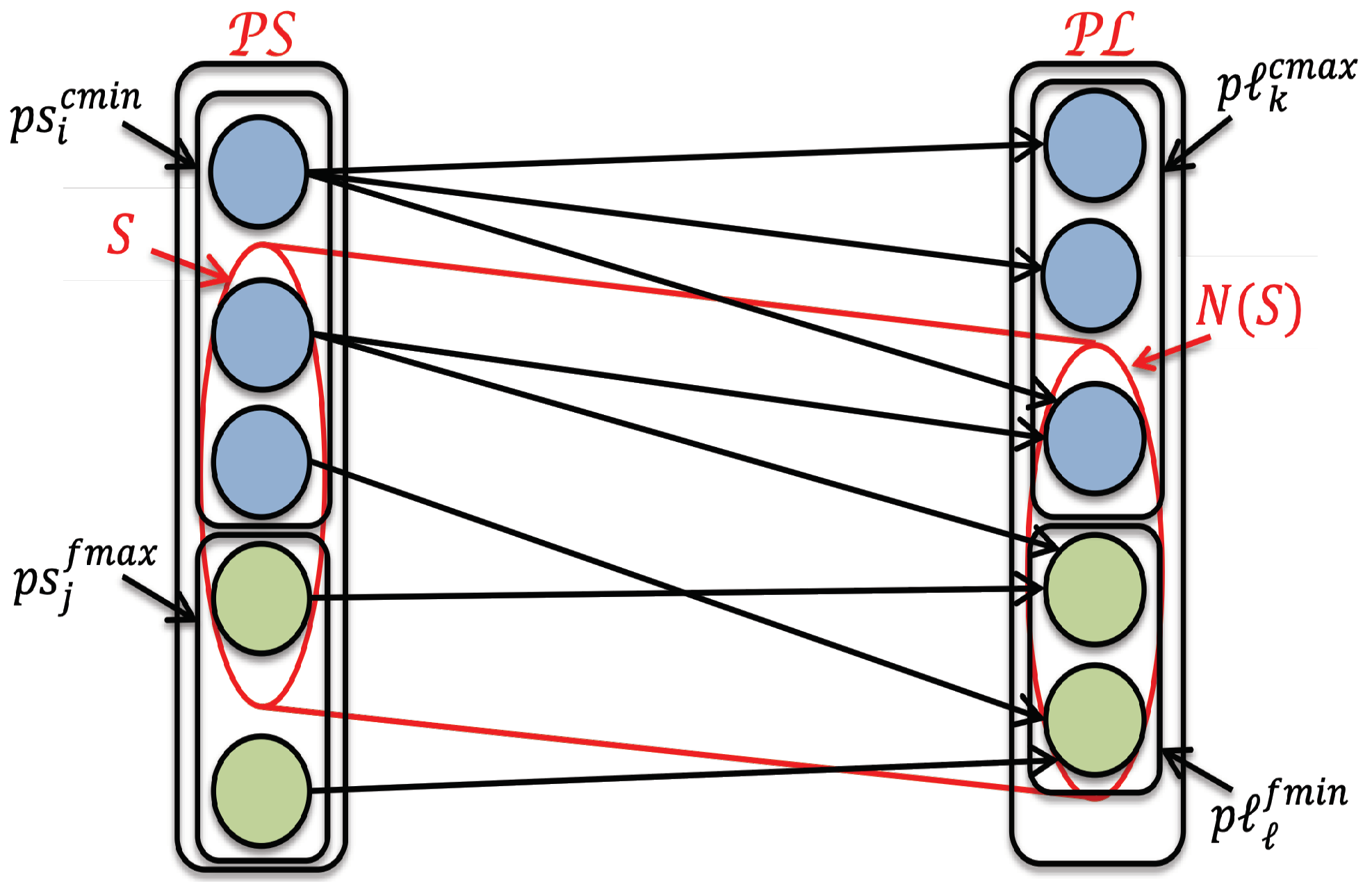
4. New Solvability Theorem

In this section, we will propose a new solvability theorem in order to identify the power system consisting of power source devices, power load devices and power flow connections with power level limitation to assure the existence solution for any value power level.
Theorem 2.
The power system always has a feasible power assignment solution for any given or measured power levels of uncontrollable devices, if and only if
Condition 2-1:
The existence of a power flow assignment x : X R + that fulfills following limitations,
P S i c , p s i c m i n = O i c
P S j f , p s j f m a x = O j f
P L k c , p k c m a x I k c
P L f , p f m i n I f
Condition 2-2:
The existence of a power flow assignment x : X R + that fulfills given limitations,
P S i c , p s i c m a x O i c
P S j f , p s j f m i n O j f
P L k c , p k c m i n = I k c
P L f , p f m a x = I f
Proof of Theorem 2.
To prove the above solvability theorem, at first, we will present the equivalences between system condition 2-1 in newly proposed theorem-2 and system condition 1-1 in theorem-1. Subsequently, we will show the correspondence between system condition 2-2 and system condition 1-2. In the beginning, we will verify the sufficiency of system condition 2-1 to system condition 1-1. Let x : X R + is a feasible power assignment solution that fulfills the following system conditions for every P S and P L .
p s i c m i n = O i c , for   each   P S i c
p s j f m a x = O j f , for   each   P S j f
p k c m a x I k c , for   each   P L k c
p f m i n I f , for   each   P L f
Now, let subset S of power source devices be a random subset and neighboring set of connected power load devices N ( S ) , then the following system condition holds as,
P S i c C ( S ) p s i c m i n + P S j f F ( S ) p s j f m a x = P S i c C ( S ) O i c + P S j f F ( S ) O j f
However, because every power source device in subset S is associated to only power load devices in neighboring subset N ( S ) , load devices in N ( S ) may have power flow connections with source devices not in S (see Figure 5). Therefore, in comparison with the total outgoing power supply from subset S of power source devices with total incoming power to power load devices in subset N ( S ) , the former must not be greater than the latter, i.e.,
P S i c C ( S ) O i c + P S j f F ( S ) O j f P L k c C ( N ( S ) ) I k c + P L f F ( N ( S ) ) I f
From Equations (17) and (18), we have
P S i c C ( S ) O i c + P S j f F ( S ) O j f P L k c C ( N ( S ) ) I k c + P L f F ( N ( S ) ) I f P L k c C ( N ( S ) ) p k c m a x + P L f F ( N ( S ) ) p f m i n
This proves the sufficiency of our system condition 2-1 to system condition 1-1. Here, we will also show the necessity of system condition 2-1 to system condition 1-1. For this, we will present an auxiliary Optimization Problem and power device definitions.
Optimization Problem for the Proof: For physical constraints of minimum and maximum power bounds of fluctuating and controllable devices, identify the power flow assignment x : X R + , such that
m i n i = 1 I p s i c m i n O i c + j = 1 J p s j f m a x O j f
with following constraints,
O i c p s i c m i n , 1 i I
O j f p s j f m a x , 1 j J
I k c p k c m a x , 1 k K
I f p f m i n , 1 L
A power flow assignment that fulfills all physical limitations is named as a feasible power solution, and a feasible power solution that minimizes the objective function is named as an optimum solution.
A source device can have three possible states, called Power-High, Power-Balanced, and Power-low.
Definition 1: [Power-High]: when p s i c m i n > O i c and p s j f m a x > O j f satisfy for P S i c and P S j f , respectively, these power source devices are named as “power-high” devices.
When I k c > p k c m a x and I f > p f m i n satisfy for P L k c and P L f , respectively, these power load devices are also termed as “power-high” devices.
[Power-Balanced]: the situation when the entire summation of all outgoing/incoming power flow connections from/to a source/load device is equal to the stated power value, p s i c m i n = O i c , p s j f m a x = O j f , I k c = p k c m a x and I f = p f m i n , the power device is entitled as “power-balanced”.
[Power-Low]: when p s i c m i n < O i c and p s j f m a x < O j f satisfy for P S i c and P S j f , respectively, and when I k c < p k c m a x and I f < p f m i n satisfy for P L k c , and P L f , respectively, these power devices are termed as “power-balanced” devices.
Definition 2: the control path is an alternative arrangement of power devices and power flow connections, when each power device in a control path is either an beginning device followed by a power flow connection incident to this power device, an intermediary power device that is incident to the previous and the next connected power flow connections or an ending power device that is incident to the previous power flow connection. The control path might comprise of “forward power flow connections” having similar direction with control path direction as well as “backward power flow connections” having the reverse direction with the control path direction. Each backward power flow connection in a control path has positive power flow, then the control path is named as “alternating control path”. The power flow requirement on each power flow connection of an alternating control path is presented in Figure 7.
Definition 3: An alternating control path that begins with a “power-high” power device and ends on a “power-low” power device is termed as an augmenting control path, as shown in (Figure 8).
Definition 4: For to an augmenting control path, the process for increasing power flow on each power flow connection in the control path equally by Δ > 0 (forward power flow +Δ, and −Δ for a backward power flow) is named “power flow modification”. Note that, in this power flow modification, the entire outgoing/incoming power changes only at a initiating power device and a terminating power device.
Please notice that, the use of words “alternating control path” and “augmenting control path” are taken from Graph Theory [35]. The control paths are just the computational steps, not the actual power flow on each connection. That is, the control path is definitely independent of the actual power flow. This idea of control path is based on purely mathematical computation.
Now, we are going to prove the necessity of system condition 2-1 to system condition 1-1. The ultimate focus of this representation is to demonstrate that Optimization Problem for this proof has an optimum power solution that can achieve the objective function equivalent to zero.
Here, we will assume that the optimum power solution x * : X R + does not satisfy the objective function equivalent to zero. That is, there exists P S a , such that O a < p s a due to the constraints (20) and (21). We consider alternating control paths initiating from P S a , and let A be the group of power source devices that is updated from P S a by alternating control paths (see Figure 9). Correspondingly, let B be the group of power load devices that can be reached from P S a by alternating control paths. Because an alternating control path can be reached from a power source device to a power load device with no limitation, B = N ( A ) . However, power load devices in B can have a power flow connection (which must have power flow as zero) with power source devices not in A, i.e., A N ( B ) . The demanded power by power load devices in B is provided from only connected source devices existing in A, since power flows on power flow connections starting with PS \ A ending on B are zero.
Now, we will consider two possible cases, as given below.
[Case-1]: At least one power device, as P L b , in B is “power-low”.
The alternating control path from P S a to P L b is an augmenting control path. Along the control path, the power flow can be augmented and the difference between p s a O a can be decreased to obtain a new power flow solution that is better than the assumed power solution x * : X R + .
[Case-2]: all of the power devices in B are “power-balanced”.
In case the load devices in B are "power-balanced" devices, this results in,
P S i c C ( A ) p s i c m i n + P S j f F ( A ) p s j f m a x > P S i c C ( A ) O i c + P S j f F ( A ) O j f = P L k c C ( N ( A ) ) I k c + P L f F ( N ( A ) ) I j f = P L k c C ( N ( A ) ) p k c m a x + P L f F ( N ( A ) ) p f m i n
which disproves system condition 1-1 in above Theorem 1.
From the case-1 and the case-2, the Optimization Problem for the proof has a power solution that proves the objective function equivalent to zero, which shows the feasible solution existence shown in condition 2-1.
In order to prove the necessity and sufficiency for system condition as given in 2-2 to system condition given in 1-2, at first, we apply interchange of power source devices and load devices (see Figure 10) so that the relation between condition 2-2 and condition 1-2 is mathematically reduced into the relation between condition 2-1 and condition 1-1.
After the interchange of power devices, the representation of power sources of both types i.e., controllable and fluctuating can be shown as PL = { P L 1 c , P L 2 c , , P L K c , P L 1 f , P L 2 f , , P L L f } = { P L 1 , P L 2 , P L 3 , , P L K + L } where K and L represent the entire group of controllable and fluctuating power sources, respectively. The minimum and maximum power supply limits for controllable power sources can be defined as p k c m i n and p k c m a x for P L k c . The power generation limitation for fluctuating power source can be defined as p f m i n and p f m a x , respectively, for P L f .
Similarly, the representation of power loads can be replaced as, PS = { P S 1 c , P S 2 c , , P S I c , P S 1 f , P S 2 f , , P S J f } = { P S 1 , P S 2 , P S 3 , , P S I + J } , where I and J represent the entire group of controllable and fluctuating power loads. The minimum power limitation and maximum power limits for controllable power loads can be defined as p s i c m i n and p s i c m a x , respectively, for P S i c . The consumption limitation can be represented as p s j f m i n and p s j f m a x for P S j f .
According to this exchange of power sources and power loads, we will consider the set of connections X ^ , such that ( P L m , P S n ) X ^ if and only if ( P S n , P L m ) X .
After interchange, the condition 1-2 can be seen as condition 1-1 for the transformed system.
T PL , P L k c C ( T ) p k c m i n + P L f F ( T ) p f m a x P S i c C ( N ( T ) ) p s i c m a x + P S j f F ( N ( T ) ) p s j f m i n
In above equation p k c m i n + p f m a x show the generated power of power sources and p s i c m a x + p s j f m i n show the power demand of power loads. From the equivalency proof of condition 1-1 to condition 2-1, a power flow assignment exists x ^ : X ^ R + , which fulfills the given system conditions for every P S and P L .
P L k c , p k c m i n = O ^ k c
P L f , p f m a x = O ^ f
P S i c , p s i c m a x I ^ i c
P S j f , p s j f m i n I ^ j f
where, O ^ k c and O ^ f show the outgoing power from controllable power sources P L k c and fluctuating power sources P L f , respectively. The incoming power flows to controllable power loads P S i c and fluctuating power loads P S j f are given as I ^ i c and I ^ j f , accordingly.
Subsequently, we return to the original system and consider power flow assignment x, such that x ( P S m , P L n ) = x ^ ( P L n , P S m ) with outgoing and incoming power flows as,
O m = P L n N ( P S m ) x ( P S m , P L n ) = P L n N ( P S m ) x ^ ( P L n , P S m ) = I ^ m
I n = P S m N ( P L n ) x ( P S m , P L n ) = P S m N ( P L n ) x ^ ( P L n , P S m ) = O ^ n
From the above, we have
P L k c , p k c m i n = O ^ k c = I k c
P L f , p f m a x = O ^ f = I f
P S i c , p s i c m a x I ^ i c = O i c
P S j f , p s j f m i n I ^ j f = O j f
which shows the equivalency of condition 2-1 to condition 2-2. □

5. Demonstrations

5.1. Example of Robustness Test

In order to test whether a power flow system under the test satisfies the conditions in Theorem-2, Linear Programming (LP) solver can be used for individually checking conditions 2-1 and 2-2. Our problem is just to identify the existence of feasible solution of a set of constraints, and objective function is not needed.
Here, we consider the power system with four power source devices and five load devices with given power flow connections (see Figure 11 for the representation of given system). Two of the power sources are selected as fluctuating sources, as, P S 1 f , P S 2 f . The remaining two power source devices are selected as controllable sources, as, P S 1 c , P S 2 c . Similarly, two of the power load devices are selected as fluctuating loads as, P L 1 f , P L 2 f . The remaining three power loads are selected as controllable loads, as, P L 1 c , P L 2 c and P L 3 c . The power supply/consumption level for all power devices (i.e., power sources and loads with both types) are bounded between maximum and minimum power limits which are shown in Figure 11 and Figure 12.
As the first step, by applying LP solver, we have confirmed that there exists a power flow assignment that satisfies condition 2-1. The solution that is obtained by the LP solver is shown in Figure 11. We can easily verify that the outgoing power from each power source is equal to its minimum power limitation for a controllable power source and its maximum power limitation for a fluctuating power source. Additionally, the incoming power is equal or less than the minimum power limitation for each fluctuating power load and the maximum power limitation for each controllable power load.
As the second step, the existence of a power flow assignment which satisfies condition 2-2 has been confirmed, as is shown in Figure 12. We can also verify that the incoming power flows to power loads are equal to the minimum power limitation for controllable power loads and maximum power limit for fluctuating power loads. As for the outgoing power flows from power sources, the power flows are equal or less than the maximum power limit of fluctuating power loads and minimum power limit for controllable loads.
From Figure 11 and Figure 12, we noticed that the conditions 2-1 and 2-2 are satisfied. Hence, it is proved that the given system is robust. In order to verify the test result that was obtained by applying Theorem-2, we have tested the robustness of the same power flow system with Theorem-1. All of the subsets/groups of power sources and neighbor subsets of power loads along with power generation and consumption computation according to condition 1-1 are shown in Table 1. For each subset of power sources, the the summation of minimum limits for controllable devices and maximum power limits for fluctuating power sources is less than or equal to the summation of maximum limits for controllable devices and minimum power limits for fluctuating power loads. Similarly, we checked all of the subsets of power loads and neighboring power sources and confirmed that the condition 1-2 is also satisfied.
Next, we show that the situation of the given system cannot guarantee the existence of feasible power flow assignment. We consider the same system discussed in Figure 11, except the maximum power limit for fluctuating power source P S 1 f . The maximum power limit is changed from P S 1 f m a x = 3 to P S 1 f m a x = 14 . With respect to the new system after changing the maximum power limit, the list of all groups/subsets of power sources with neighboring subsets/groups power loads are generated along with generation and consumption computation for condition 1-1. Among them, the subset { P S 1 f } and neighbor subset of power loads { P L 3 c , P L 1 f } , the condition 1-1 is not satisfied, as shown in Table 2.
On the other hand, if we apply Theorem-2 to this new power flow system, then we can find that there is no assignment of power flow that meets the condition 2-1, since the constraint (8) requests; O 1 f = x ( P S 1 f , P L 3 c ) + x ( P S 1 f , P L 1 f ) = p s 1 f m a x = 14 and constraints (9) and (10) request; x ( P S 1 f , P L 3 c ) I 3 c p 3 c m a x = 12 , and x ( P S 1 f , P L 1 f ) I 1 f p 1 f m i n = 1 , but these three equations cannot hold simultaneously.

5.2. Comparison between Theoretical Result and Monte Carlo Simulation

In this subsection, our theoretical result (the result of applying Theorem 2) will be verified by Monte Carlo Simulation. As for a system to be tested, we consider a power system that consists of five controllable power sources, five fluctuating power sources, five controllable power loads, and five fluctuating power loads with individual minimum and maximum power level limitations shown in Table 3. As we have assumed in this paper, each fluctuating power source/load will take any power level within the given minimum and maximum bounds, which is uncontrollable for a power flow controller. On the other hand, the power level of a controllable power source/load can be controlled by the power flow controller, but the controlled value must be within the given minimum and maximum power limits.
If all power sources and loads are connected in such a way that the power can be supplied from every one of power sources to any one of power loads, i.e., the connections can be modeled with a complete bipartite graph, then the robustness condition (Theorem 1) is satisfied, and the system has always a feasible solution about the power flow assignment to connections so that the power balance is achieved and the power levels of controllable power sources/loads stay within the specified ranges.
Now, we suppose that the power flow from power sources to loads are limited, as shown in Figure 13 (System-1). At first, we have applied Theorem 2 to this power system, and found that two test power flow assignment problems (i.e., condition 2-1 and condition 2-2) have feasible solutions given in Table 4 and Table 5. Hence, we can conclude that the system always has a feasible power flow assignment solution for any given power value of fluctuating power devices. The Monte Carlo Simulation has been applied in order to verify this conclusion. In this simulation, we have generated 1,000,000 vector patterns of power levels of fluctuating power devices (each vector pattern is ( p s 1 f , , p s 5 f , p 1 f , , p 5 f ) ), and solved 1,000,000 instances of the power flow assignment problem. Finally we verified that all of these 1,000,000 problem instances have feasible solutions.
From the first solution Table 4 for condition 2-1, we found that we can relax the minimum possible power level of P L 4 f from 100 to 75, since, even if we change it, we still have the same solution with the previous one, and the new system still satisfies Theorem 1. Similarly, from the second solution Table 5 for condition 2-2, we can grade down the maximum generating power levels for P S 1 c , P S 4 c and P S 5 c from 160 to 153, from 100 to 90 and from 100 to 92, respectively, while keeping the robustness against fluctuations. The Monte Carlo Simulation has also been applied to this new system (System-2), and it has been verified that 1,000,000 problem instances have feasible solutions.
If we reduce the maximum power level for P S 5 c further from 92 to 90, the system does not satisfies Theorem 2, and the Monte Carlo Simulation shows that 332 instances out of 1,000,000 instances fail to find feasible solutions. When compared with the case of P S 5 c , if we reduce the maximum power level of P S 2 c from 100 to 90 from System-2, the resultant system does not satisfy Theorem 2 again, but its impact to the degradation of robustness is smaller, since only 16 instances out of 1,000,000 instances fail to find feasible solution.
Removing some connections/power flows between sources and loads may also degrade the robustness against power fluctuations. For example, if we remove a connection between P S 2 f and P L 4 f from power system-2, then the resultant power system does not satisfy Theorem 2, and Monte Carlo Simulation reports that 163,802 instances out of 1,000,000 instances fail to find feasible solution.

5.3. Comparison with Our Previous Method

The issue of time complexity is discussed in this subsection in order to show the comparison between new approach presented in this paper and our previous paper [27].
If we apply Theorem-1 for testing whether a given system possesses the robustness against fluctuation or not, we need to generate all subsets of the set of power sources PS (and all subsets of power loads PL as well). Because there exist 2 | PS | subsets of PS , the time complexity for the testing is no smaller than the order 2 | PS | . For example, suppose that a power flow system has 100 power sources, and the inequality condition 1-1 for one subset S of power sources can be checked with one cycle of a CPU operating with 5 GHz clock. That is, 5 × 10 9 2 32 subsets can be tested for inequality in one second. Because 2 100 different subsets exist, in order to complete the test, 2 100 / 2 32 = 2 68 s (approximately 9.4 × 10 12 years) are needed.
Table 6 shows the comparison of real computation times of robustness tests based on Theorem 1 and Theorem 2. In this experiment, we have developed Theorem 1 based and Theorem 2 based robustness test programs, which are written with C-language and executed on Linux operating system with CPU Core I7, 16GB memory. We have generated multiple power flow system configurations, and measured the computation time by applying the test program to each instance of power flow system. The computation time that is shown in the table is an average of three trials with three different instances having the same size.
Through this experiment, a remarkable improvement in the computation time for the robustness test achieved by Theorem 2 has been verified.

6. Concluding Remarks

Renewable power sources, such as photo-voltaic and wind power generation systems, can play extremely significant roles in power systems due to their low impact on the environment. However, the output power fluctuations from these energy sources alters dynamically, thus resulting in high risk of power fluctuations that is not controllable. Due to the intermittence and variability of these power sources, the power grid is facing challenges that are related to power system steady operations.
Furthermore, the power fluctuations that are triggered by power load devices have similar effects on power system. In this context, where power generation and consumption changes dynamically, a power flow control method is presented. The proposed power flow control finds power levels for controllable devices and power flow connections between devices to manage power fluctuations. This paper presents a new robustness method that comprises of both controllable and fluctuating devices and can ensure the existence of power flow assignment of power devices and power flow connections for any value of fluctuating devices. In this paper, the proposed robustness method can be expressed as a linear problem, which can be solved with respect to polynomial time complexity. This paper is a first attempt to study the structural conditions for solvability. The consideration of power loss issue and capacity of individual connection remain as future problem.

Author Contributions

Conceptualization, S.J., M.K, and Y.T.; writing–original draft preparation, S.J.; writing–review and editing, S.J., and M.K.; supervision, M.K., Y.T. All authors have read and agreed to the published version of the manuscript.

Funding

This research received no external funding.

Conflicts of Interest

The authors declare no conflict of interest.

Appendix A

Structural Power-Balancing Condition in Theorem-1 consists of condition 1-1 and condition 1-2, where 1-1 is related to one side of power-balancing that the power generated by power sources is fully consumed, while 1-2 is related to the other side that the power demanded by power loads is fully supplied.
At first, condition 1-1 is reviewed for its necessity. When we consider an arbitrary subset S of power sources, the overall power P S m S p s m generated by S is sent only to its neighbors N ( S ) , while power loads in N ( S ) receive power not only from S but also from N ( N ( S ) ) \ S (note that N ( N ( S ) ) S ) see Figure A1. That is, the overall power which N ( S ) receives is no smaller than the overall power which is sent out from S. Since the overall demand P L n N ( S ) p n of power loads in N ( S ) is equivalent to the power which N ( S ) receives, the following inequality holds.
P S m S p s m P L n N ( S ) p n
With respect to a controllable source P S i c in the set S, we can control its generating power level within the available range [ p s i c m i n , p s i c m a x ] . In order for the system to possess a solution satisfying the above inequality with the specified control range of each controllable power source, the inequality must hold with the minimum power level p s i c m i n for p s m of each controllable power source. Similarly, with respect to a controllable load P L k c in the set N ( S ) , the above inequality must hold with the maximum demand level p k c m a x for p n of each controllable power load.
On the other hand, with respect to a fluctuating power source P S j f in S, we cannot control its power level, and hence we need to consider the worst case. Considering the above inequality, the worst case arises when the generated power level is maximum. Similarly, with respect to a fluctuating power load, the worst case arises when the demand level is minimum.
Finally, we can conclude that, for a system to have a power-balanced solution in any situation of fluctuating devices, the above inequality must hold in the following form (condition 1-1);
P S i c S p s i c m i n + P S j f S p s j f m a x P L k c N ( S ) p k c m a x + P L f N ( S ) p c m i n
Figure A1. An example of subset S and its neighbor N ( S ) .
Designs 04 00048 g0a1
Next, condition 1-2 is reviewed for its necessity. When we consider an arbitrary subset T of power loads, the overall power provided to T comes only from the neighbors of T, N ( T ) , while N ( T ) provides power not only to T but also to power loads in N ( N ( T ) ) \ T , where N ( N ( T ) ) T . Hence, the overall generated power by N ( T ) is no smaller than the overall power provided to T. As a result, the following inequality holds.
P S m N ( T ) p s m P L n T p n
Similar to the previous review for condition 1-1, with respect to the above inequality, we can consider the best possible case for controllable sources and loads (replacing p s m with p s i c m a x for each controllable source in N ( T ) and replacing p n with p k c m i n for each controllable load in T), and we need to consider the worst case for fluctuating sources and loads (replacing p s m with p s j c m i n for each fluctuating source in N ( T ) and replacing p n with p f m a x ). Finally, the above inequality must hold in the following form (Condition 1-2);
P S i c S p s i c m a x + P S j f S p s j f m i n P L k c N ( S ) p k c m i n + P L f N ( S ) p c m a x
For more detailed explanation and mathematical proof, especially for the sufficiency of the condition, please refer to [27].

References

  1. Soroudi, A.; Ehsan, M.; Caire, R.; Hadjsaid, N. Possibilistic evaluation of distributed generations impacts on distribution networks. IEEE Trans. Power Syst. 2011, 26, 2293–2301. [Google Scholar] [CrossRef] [Green Version]
  2. Majd, A.A.; Farjah, E.; Rastegar, M. Composite generation and transmission expansion planning toward high renewable energy penetration in Iran power grid. IET Renew. Power Gener. 2020, 14, 1520–1528. [Google Scholar] [CrossRef]
  3. Maegaard, P. Balancing fluctuating power sources. In Proceedings of the World-Non-Grid-Connected Wind Power and Energy Conference, Nanjing, China, 5–7 November 2010. [Google Scholar]
  4. Umer, S.; Tan, Y.; Lim, A.O. Stability analysis for smart homes energy management system with delay consideration. J. Clean Energy Technol. 2014, 2, 332–338. [Google Scholar] [CrossRef]
  5. Umer, S.; Tan, Y.; Lim, A.O. Priority based power sharing scheme for power consumption control in smart homes. Int. J. Smart Grid Clean Energy 2014, 3, 340–346. [Google Scholar] [CrossRef] [Green Version]
  6. Umer, S.; Kaneko, M.; Tan, Y.; Lim, A.O. System design and analysis for maximum consuming power control in smart house. J. Autom. Control Eng. 2014, 2, 43–48. [Google Scholar] [CrossRef]
  7. Kumar, G.A.; Sujay, N.; Tejas, P.; Srikanth, P.; Yashavanth, T.R. Design and implementation of wireless sensor network based smart DC grid for smart cities. In Proceedings of the 4th International Conference on Recent Trends on Electronics, Information, Communication and Technology (RTEICT), Bangalore, India, 17–18 May 2019; pp. 1453–1458. [Google Scholar]
  8. Lumbreras, S.; Ramos, A.; Banez-Chicharro, F. Optimal transmission network expansion planning in real-sized power systems with high renewable penetration. Electr. Power Syst. Res. 2017, 149, 76–88. [Google Scholar] [CrossRef]
  9. Shalukho, A.V.; Lipuzhin, I.A.; Voroshilov, A.A. Power quality in microgrids with distributed generation. In Proceedings of the International Ural Conference on Electric Power Engineering (UralCon), Chelyabinsk, Russia, 1–3 October 2019; pp. 54–58. [Google Scholar]
  10. Han, J.; Choi, C.; Park, W.; Lee, I.; Kim, S. Smart home energy management system including renewable energy based on ZigBee and PLC. IEEE Trans. Consum. Electron. 2014, 60, 198–202. [Google Scholar] [CrossRef]
  11. Han, J.; Choi, C.; Park, W.; Lee, I.; Kim, S. PLC-based photovoltaic system management for smart home energy management system. IEEE Trans. Consum. Electron. 2014, 60, 184–189. [Google Scholar] [CrossRef]
  12. Hong, I.; Kang, B.; Park, S. Design and implementation of intelligent energy distribution management with photovoltaic system. IEEE Trans. Consum. Electron. 2012, 58, 340–346. [Google Scholar] [CrossRef]
  13. Rashidi, Y.; Moallem, M.; Vojdani, S. Wireless Zigbee system for performance monitoring of photovoltaic panels. In Proceedings of the 2011 37th IEEE Photovoltaic Specialists Conference, Seattle, WA, USA, 19–24 June 2011; pp. 3205–3207. [Google Scholar]
  14. Xiaoli, X.; Daoe, Q. Remote monitoring and control of photovoltaic system using wireless sensor network. In Proceedings of the International Conference on Electric Information and Control Engineering, Wuhan, China, 15–17 April 2011; pp. 633–638. [Google Scholar]
  15. Biabani, M.; Golkar, M.A.; Johar, A.; Johar, M. Propose a home demand -side management algorithm for smart nano-grid. In Proceedings of the 4th Annual International Power Electronics, Drive Systems and Technologies Conference, Tehran, Iran, 13–14 February 2013; pp. 487–494. [Google Scholar]
  16. Asare-Bediako, B.; Kling, W.L.; Ribeiro, P.F. Home energy management systems: Evolution, trends and frameworks. In Proceedings of the 2012 47th International Universities Power Engineering Conference (UPEC), London, UK, 4–7 September 2012; pp. 1–5. [Google Scholar]
  17. Shwehdi, M.H.; Mohamed, S.R. Proposed smart DC Nano-Grid for green buildings a reflective view. In Proceedings of the 2014 International Conference on Renewable Energy Research and Application (ICRERA), Milwaukee, WI, USA, 19–22 October 2014; pp. 765–769. [Google Scholar]
  18. Kinn, M.C. Proposed components for the design of a smart Nano-Grid for a domestic electrical system that operates at below 50V DC. In Proceedings of the 2011 2nd IEEE PES International Conference and Exhibition on Innovative Smart Grid Technologies, Manchester, UK, 5–7 December 2011; pp. 1–7. [Google Scholar]
  19. Schonberger, J.; Duke, R.; Round, S.D. DC-Bus signaling: A distributed control strategy for a hybrid renewable Nano-grid. IEEE Trans. Ind. Electron. 2006, 53, 1453–1460. [Google Scholar] [CrossRef]
  20. Latha, S.H.; Mohan, S.C. Centralized power control strategy for 25 kW Nano-Grid for rustic electrification. In Proceedings of the 2012 International Conference on Emerging Trends in Science, Engineering and Technology (INCOSET), Tiruchirappalli, India, 13–14 December 2012; pp. 666–669. [Google Scholar]
  21. He, L.; Wei, Z.; Yan, H.; Xv, K.Y.; Zhao, M.Y.; Cheng, S. A day ahead scheduling optimization model of multi-microgrid considering interactive power control. In Proceedings of the International Conference on Intelligent Green Building and Smart Grid (IGBSG), Yi-chang, China, 6–9 September 2019; pp. 456–461. [Google Scholar]
  22. Kondoh, J.; Higuchi, N.; Sekine, S.; Yamaguchi, H.; Ishii, I. Distribution system research with an analog simulator. In Proceedings of the Power Electronics for Distributed and Co-Generation, Irvine, CA, USA, 22–24 March 2004. [Google Scholar]
  23. Kondoh, J.; Aki, H.; Yamaguchi, H.; Murata, A.; Ishii, I. Consumed power control of time deferrable loads for frequency regulation. In Proceedings of the IEEE PES Power Systems Conference and Exposition, New York, NY, USA, 10–13 October 2004. [Google Scholar]
  24. Javaid, S.; Kurose, Y.; Kato, T.; Matsuyama, T. Cooperative distributed control implementation of the power flow coloring over a Nano-grid with fluctuating power loads. IEEE Trans. Smart Grid 2017, 8, 342–352. [Google Scholar] [CrossRef]
  25. Javaid, S.; Kato, T.; Matsuyama, T. Power flow coloring system over a Nano-grid with fluctuating power sources and loads. IEEE Trans. Ind. Inf. 2017, 13, 3174–3184. [Google Scholar] [CrossRef]
  26. Yamaguchi, H.; Kondoh, J.; Aki, H.; Murata, A.; Ishii, I. Power fluctuation analysis of distribution network introduced a large number of photovoltaic generation system. In Proceedings of the 18th International Conference on Electricity Distribution, Turin, Italy, 6–9 June 2005. [Google Scholar]
  27. Javaid, S.; Kaneko, M.; Tan, Y. Structural condition for controllable power flow system containing controllable and fluctuating power devices. Energies 2020, 13, 1627. [Google Scholar] [CrossRef] [Green Version]
  28. Javaid, S.; Kaneko, M.; Yasuo, T.A.N. Power flow management: Solvability condition for a system with controllable and fluctuating devices. In Proceedings of the 11th IEEE PES Asia-Pacific Power and Energy Engineering Conference (IEEE APPEEC 2019), Macao, China, 1–4 December 2019. [Google Scholar]
  29. Riffonneau, Y.; Bacha, S.; Ploix, S. Optimal power flow management for grid connected PV systems with batteries. IEEE Trans. Sust. Energy 2011, 2, 309–320. [Google Scholar] [CrossRef]
  30. Denholma, P.; Margolis, R.M. Evaluating the limits of solar pho-tovoltaics (PV) in electric power systems utilizing energy storage and other enabling technologies. Energy Policy 2007, 35, 4424–4433. [Google Scholar] [CrossRef]
  31. Perrin, M.; Saint-Drenan, Y.M.; Mattera, F.; Malbranche, P. Lead- acid batteries in stationary applications: Competitors and new markets for large penetration of renewable energies. J. Power Sources 2005, 144, 402–410. [Google Scholar] [CrossRef]
  32. Martinez Cesena, E.A.; Capuder, T.; Mancarella, P. Flexible distributed multienergy generation system expansion planning under uncertainty. IEEE Trans. Smart Grid 2016, 7, 348–357. [Google Scholar] [CrossRef]
  33. Wei, J.; Zhang, Y.; Wang, J.; Cao, X.; Khan, M.A. Multi-period planning of multi-energy microgrid with multi-type uncertainties using chance constrained information gap decision method. Appl. Energy 2020, 260, 1–19. [Google Scholar] [CrossRef]
  34. Louie, H. Off-Grid Electrical Systems in Developing Countries; Chapter 10; Springer Nature: Basel, Switzerland, 2018. [Google Scholar]
  35. Axler, S.; Ribet, K.A. Graduate Texts in Mathematics; Springer-Verlag: Berlin, Germany, 2008. [Google Scholar]
Figure 1. Illustration and categorization of power source devices, power load devices, and power flow connections between them as a bipartite graph.
Designs 04 00048 g001
Figure 2. Real physical setup example demonstration [25], reuse with permission from Saher Javaid, Power flow coloring system over a Nano-grid with fluctuating power sources and loads; published by IEEE Transactions on Industrial Informatics, 2017.
Designs 04 00048 g002
Figure 3. Physical setup example [25], reuse with permission from Saher Javaid, Power flow coloring system over a Nano-grid with fluctuating power sources and loads; published by IEEE Transactions on Industrial Informatics, 2017.
Designs 04 00048 g003
Figure 4. Power Flow Connections between Source Devices and Load Devices.
Designs 04 00048 g004
Figure 5. Representation of a subset of power source devices S and connected subset of power load devices N ( S ) .
Designs 04 00048 g005
Figure 6. Representation of a subset of power source devices T and neighboring connected power load devices N ( T ) .
Designs 04 00048 g006
Figure 7. Alternating Control Path.
Designs 04 00048 g007
Figure 8. Augmenting Control Path.
Designs 04 00048 g008
Figure 9. Representation of sets A and B of power source devices and power load devices.
Designs 04 00048 g009
Figure 10. Interchange of power source devices and power load devices.
Designs 04 00048 g010
Figure 11. Example demonstration for existence of power flow assignment, which satisfies condition 2-1.
Designs 04 00048 g011
Figure 12. Example demonstration for existence of power flow assignment that satisfies condition 2-2.
Designs 04 00048 g012
Figure 13. Power flow system with incomplete connections.
Designs 04 00048 g013
Table 1. List of all possible subsets S of PS and N ( S ) of PL .
S N ( S ) ps i cmin + ps j fmax p k cmax + p fmin
{ P S 1 c } { P L 1 c , P L 2 c , P L 3 c } 037
{ P S 2 c } { P L 2 c , P L 1 f , P L 2 f } 013
{ P S 1 f } { P L 3 c , P L 1 f } 313
{ P S 2 f } { P L 3 c , P L 1 f } 1013
{ P S 1 c , P S 2 c } { P L 1 c , P L 2 c , P L 3 c , P L 1 f , P L 2 f } 040
{ P S 1 c , P S 1 f } { P L 1 c , P L 2 c , P L 3 c , P L 1 f } 338
{ P S 1 c , P S 2 f } { P L 1 c , P L 2 c , P L 3 c , P L 1 f } 1038
{ P S 2 c , P S 1 f } { P L 2 c , P L 3 c , P L 1 f , P L 2 f } 325
{ P S 2 c , P S 2 f } { P L 2 c , P L 3 c , P L 1 f , P L 2 f } 1025
{ P S 1 f , P S 2 f } { P L 3 c , P L 1 f } 1313
{ P S 1 c , P S 2 c , P S 1 f } { P L 1 c , P L 2 c , P L 3 c , P L 1 f , P L 2 f } 340
{ P S 1 c , P S 2 c , P S 2 f } { P L 1 c , P L 2 c , P L 3 c , P L 1 f , P L 2 f } 1040
{ P S 1 c , P S 1 f , P S 2 f } { P L 1 c , P L 2 c , P L 3 c , P L 1 f } 1338
{ P S 2 c , P S 1 f , P S 2 f } { P L 2 c , P L 3 c , P L 1 f , P L 2 f 1325
{ P S 1 c , P S 2 c , P S 1 f , P S 2 f } { P L 1 c , P L 2 c , P L 3 c , P L 1 f , P L 2 f } 1340
Table 2. Partial List of subset S of PS and N ( S ) of PL .
S N ( S ) ps i cmin + ps j fmax p k cmax + p fmin
{ P S 1 c } { P L 1 c , P L 2 c , P L 3 c } 037
{ P S 2 c } { P L 2 c , P L 1 f , P L 2 f } 013
{ P S 1 f } { P L 3 c , P L 1 f } 1413
Table 3. List of power source and load devices with minimum and maximum power limitations.
Power SourcesMinimum Power LimitationMaximum Power LimitationPower LoadsMinimum Power LimitationMaximum Power Limitation
P S 1 c 0160 P L 1 c 150200
P S 2 c 0100 P L 2 c 1010
P S 3 c 0100 P L 3 c 1015
P S 4 c 0100 P L 4 c 1020
P S 5 c 0100 P L 5 c 1024
P S 6 f 60150 P L 6 f 07
P S 7 f 030 P L 7 f 056
P S 8 f 045 P L 8 f 05
P S 9 f 05 P L 9 f 100333
P S 10 f 043 P L 10 f 04
Table 4. Solution for power flow assignment for condition 2-1.
Outgoing Power from Power SourcesOutgoing PowerIncoming Power of Power LoadsIncoming Power
O 1 c 0 I 1 c 174
O 2 c 0 I 2 c 0
O 3 c 0 I 3 c 0
O 4 c 0 I 4 c 0
O 5 c 0 I 5 c 24
O 6 f 150 I 6 f 0
O 7 f 30 I 7 f 0
O 8 f 45 I 8 f 0
O 9 f 5 I 9 f 75
O 10 f 43 I 10 f 0
Table 5. Solution for power flow assignment for condition 2-2.
Outgoing Power from Power SourcesOutgoing PowerIncoming Power of Power LoadsIncoming Power
O 1 c 153 I 1 c 150
O 2 c 100 I 2 c 10
O 3 c 100 I 3 c 10
O 4 c 90 I 4 c 10
O 5 c 92 I 5 c 10
O 6 f 60 I 6 f 7
O 7 f 0 I 7 f 56
O 8 f 0 I 8 f 5
O 9 f 0 I 9 f 333
O 10 f 0 I 10 f 4
Table 6. Computation Time.
Size ( PS , PL ) Theorem 1 Based TestTheorem 2 Based Test
10, 100.000850.00035
20, 201.560.00073
25, 2560.320.00092
30, 301586.640.00113
100, 100N/A0.00400
1000, 1000N/A0.03485
Publisher’s Note: MDPI stays neutral with regard to jurisdictional claims in published maps and institutional affiliations.

