In this section, we will propose a new solvability theorem in order to identify the power system consisting of power source devices, power load devices and power flow connections with power level limitation to assure the existence solution for any value power level.
Proof of Theorem 2. To prove the above solvability theorem, at first, we will present the equivalences between system condition
2-1 in newly proposed theorem-2 and system condition
1-1 in theorem-1. Subsequently, we will show the correspondence between system condition
2-2 and system condition
1-2. In the beginning, we will verify the sufficiency of system condition
2-1 to system condition
1-1. Let
is a feasible power assignment solution that fulfills the following system conditions for every
and
.
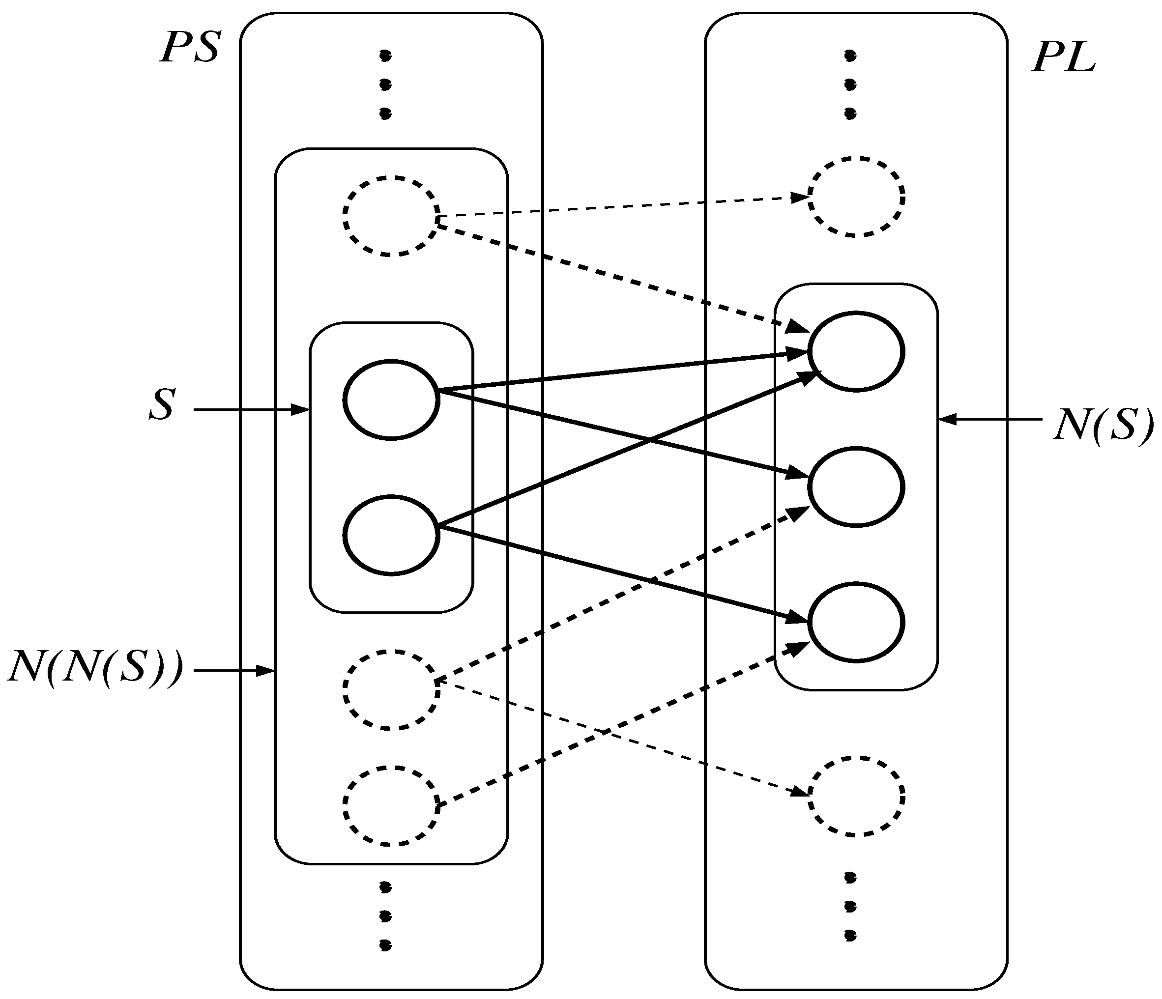
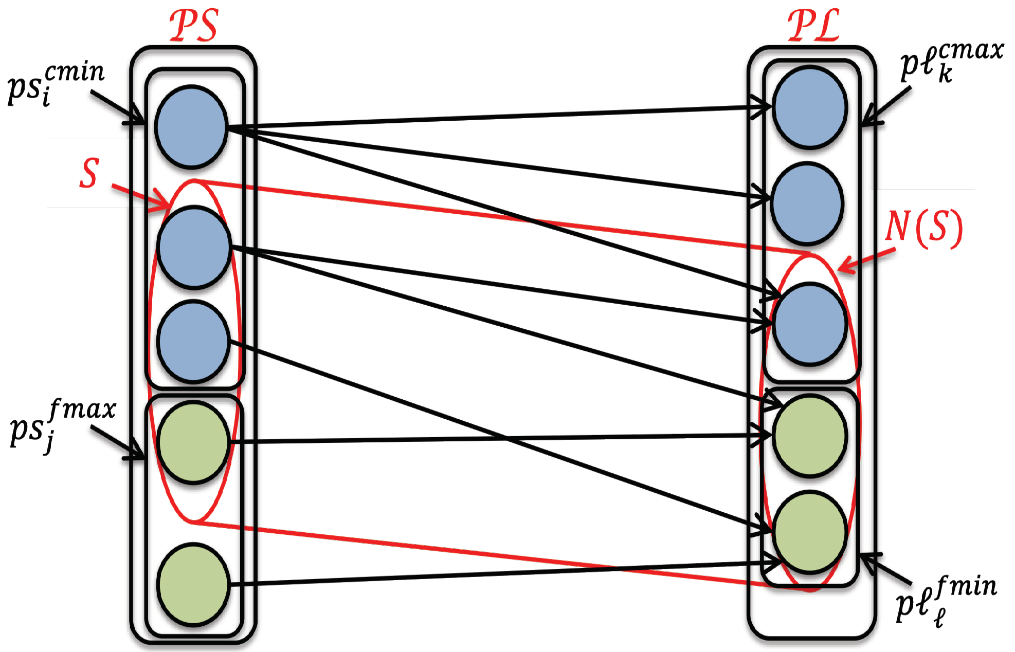
Now, let subset
S of power source devices be a random subset and neighboring set of connected power load devices
, then the following system condition holds as,
However, because every power source device in subset
S is associated to only power load devices in neighboring subset
, load devices in
may have power flow connections with source devices not in
S (see
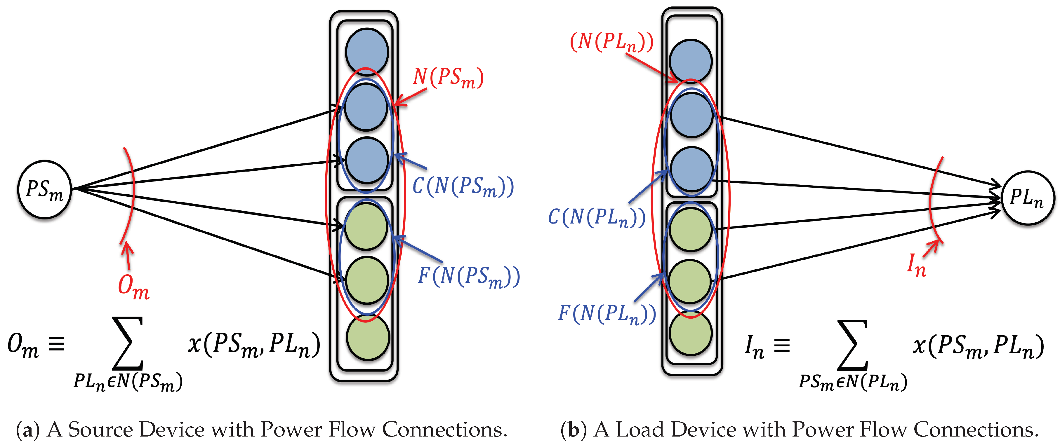
Figure 5). Therefore, in comparison with the total outgoing power supply from subset
S of power source devices with total incoming power to power load devices in subset
, the former must not be greater than the latter, i.e.,
From Equations (
17) and (
18), we have
This proves the sufficiency of our system condition 2-1 to system condition 1-1. Here, we will also show the necessity of system condition 2-1 to system condition 1-1. For this, we will present an auxiliary Optimization Problem and power device definitions.
Optimization Problem for the Proof: For physical constraints of minimum and maximum power bounds of fluctuating and controllable devices, identify the power flow assignment
, such that
with following constraints,
A power flow assignment that fulfills all physical limitations is named as a feasible power solution, and a feasible power solution that minimizes the objective function is named as an optimum solution.
A source device can have three possible states, called Power-High, Power-Balanced, and Power-low.
Definition 1: [Power-High]: when and satisfy for and , respectively, these power source devices are named as “power-high” devices.
When and satisfy for and , respectively, these power load devices are also termed as “power-high” devices.
[Power-Balanced]: the situation when the entire summation of all outgoing/incoming power flow connections from/to a source/load device is equal to the stated power value, , , and , the power device is entitled as “power-balanced”.
[Power-Low]: when and satisfy for and , respectively, and when and satisfy for , and , respectively, these power devices are termed as “power-balanced” devices.
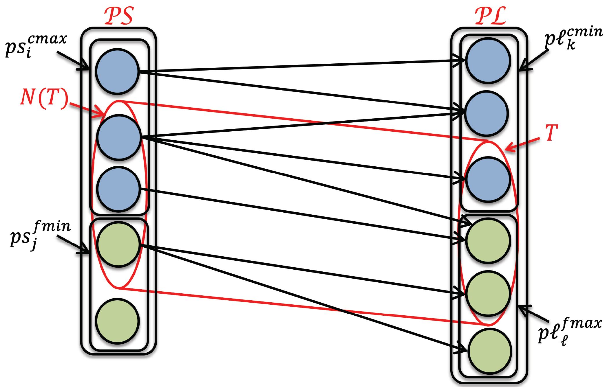
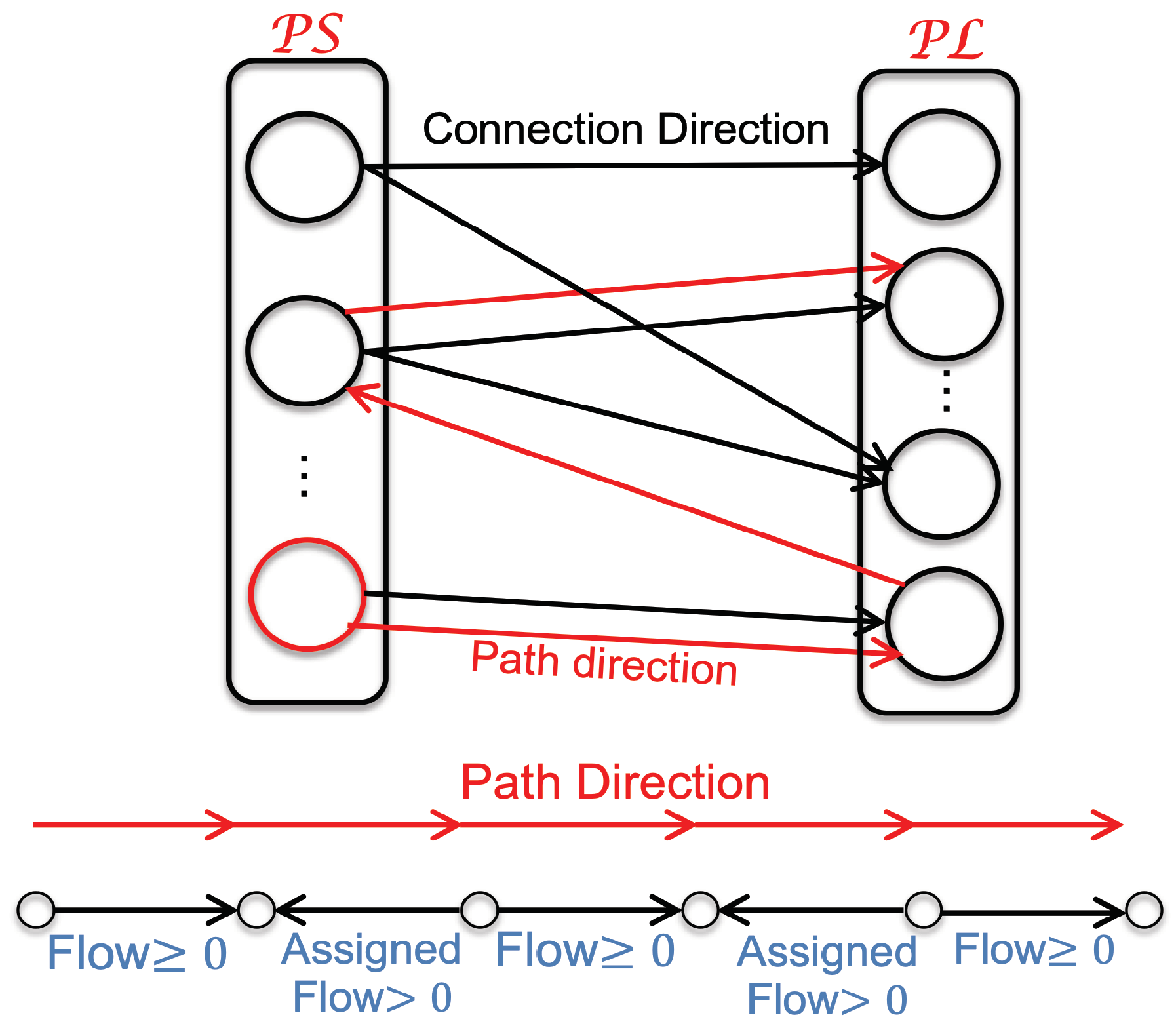
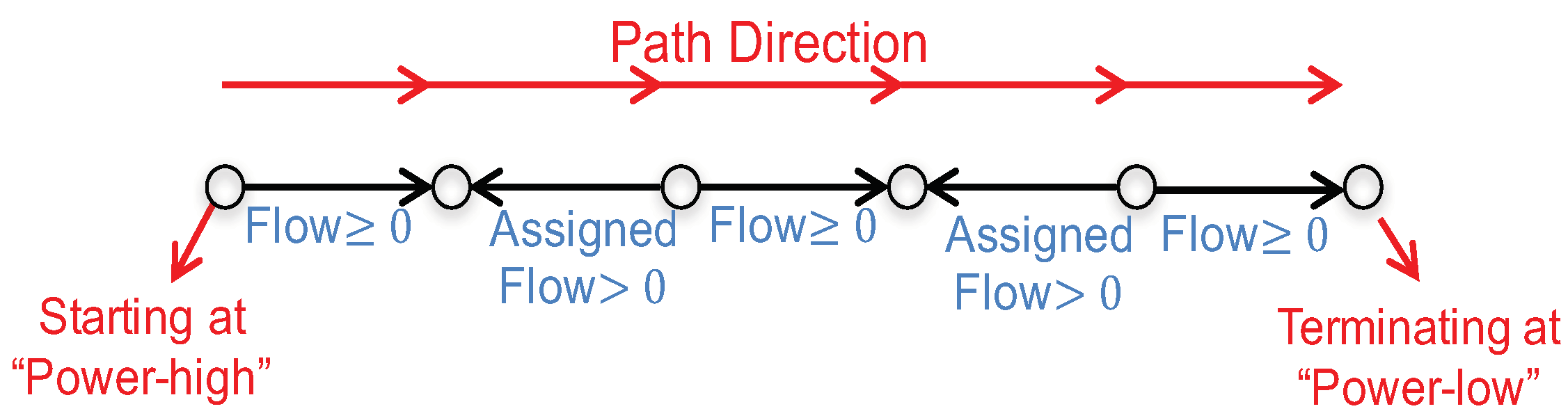
Definition 2: the control path is an alternative arrangement of power devices and power flow connections, when each power device in a control path is either an beginning device followed by a power flow connection incident to this power device, an intermediary power device that is incident to the previous and the next connected power flow connections or an ending power device that is incident to the previous power flow connection. The control path might comprise of “forward power flow connections” having similar direction with control path direction as well as “backward power flow connections” having the reverse direction with the control path direction. Each backward power flow connection in a control path has positive power flow, then the control path is named as “alternating control path”. The power flow requirement on each power flow connection of an alternating control path is presented in
Figure 7.
Definition 3: An alternating control path that begins with a “power-high” power device and ends on a “power-low” power device is termed as an augmenting control path, as shown in (
Figure 8).
Definition 4: For to an augmenting control path, the process for increasing power flow on each power flow connection in the control path equally by (forward power flow +Δ, and −Δ for a backward power flow) is named “power flow modification”. Note that, in this power flow modification, the entire outgoing/incoming power changes only at a initiating power device and a terminating power device.
Please notice that, the use of words “alternating control path” and “augmenting control path” are taken from Graph Theory [
35]. The control paths are just the computational steps, not the actual power flow on each connection. That is, the control path is definitely independent of the actual power flow. This idea of control path is based on purely mathematical computation.
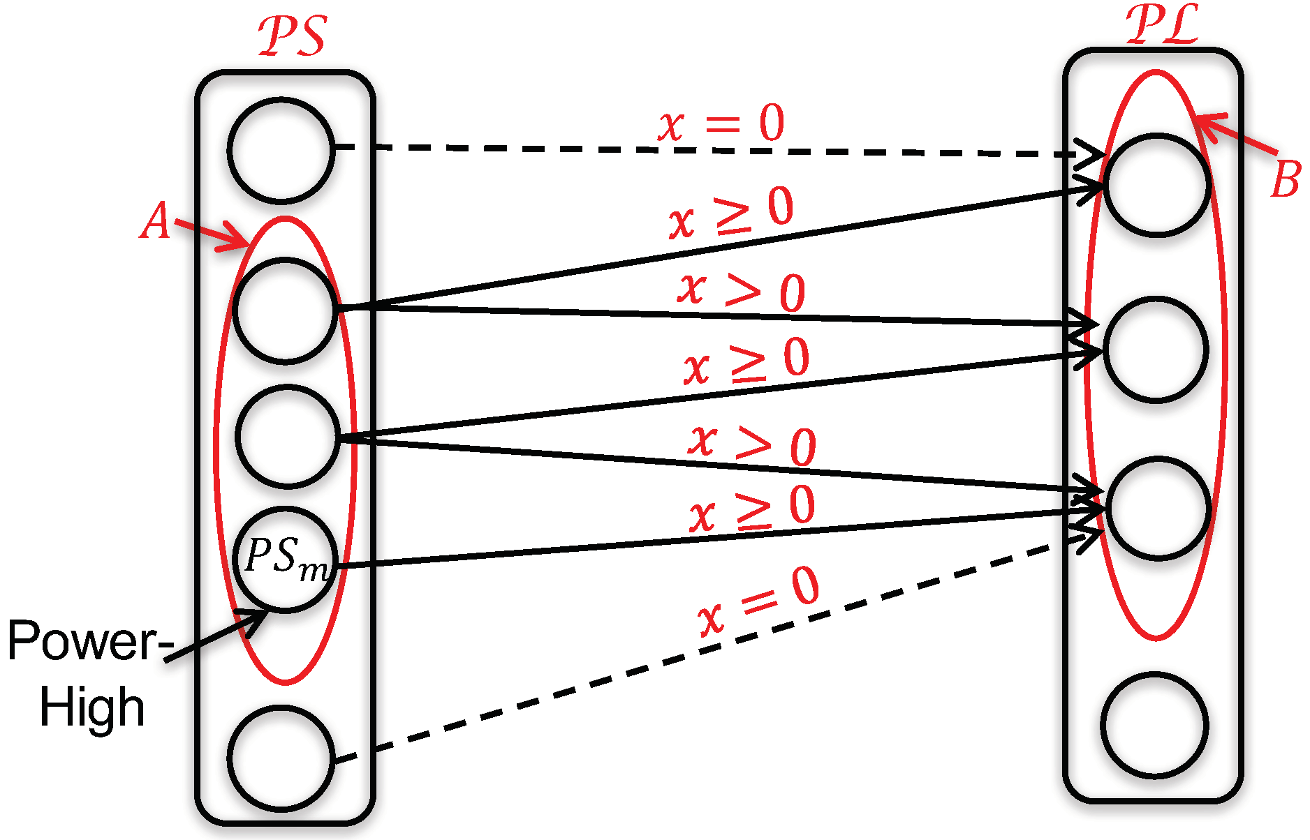
Now, we are going to prove the necessity of system condition 2-1 to system condition 1-1. The ultimate focus of this representation is to demonstrate that Optimization Problem for this proof has an optimum power solution that can achieve the objective function equivalent to zero.
Here, we will assume that the optimum power solution
does not satisfy the objective function equivalent to zero. That is, there exists
, such that
due to the constraints (
20) and (
21). We consider alternating control paths initiating from
, and let
A be the group of power source devices that is updated from
by alternating control paths (see
Figure 9). Correspondingly, let
B be the group of power load devices that can be reached from
by alternating control paths. Because an alternating control path can be reached from a power source device to a power load device with no limitation,
. However, power load devices in
B can have a power flow connection (which must have power flow as zero) with power source devices not in
A, i.e.,
. The demanded power by power load devices in
B is provided from only connected source devices existing in
A, since power flows on power flow connections starting with
ending on
B are zero.
Now, we will consider two possible cases, as given below.
[Case-1]: At least one power device, as , in B is “power-low”.
The alternating control path from to is an augmenting control path. Along the control path, the power flow can be augmented and the difference between can be decreased to obtain a new power flow solution that is better than the assumed power solution .
[Case-2]: all of the power devices in B are “power-balanced”.
In case the load devices in
B are "power-balanced" devices, this results in,
which disproves system condition 1-1 in above Theorem 1.
From the case-1 and the case-2, the Optimization Problem for the proof has a power solution that proves the objective function equivalent to zero, which shows the feasible solution existence shown in condition 2-1.
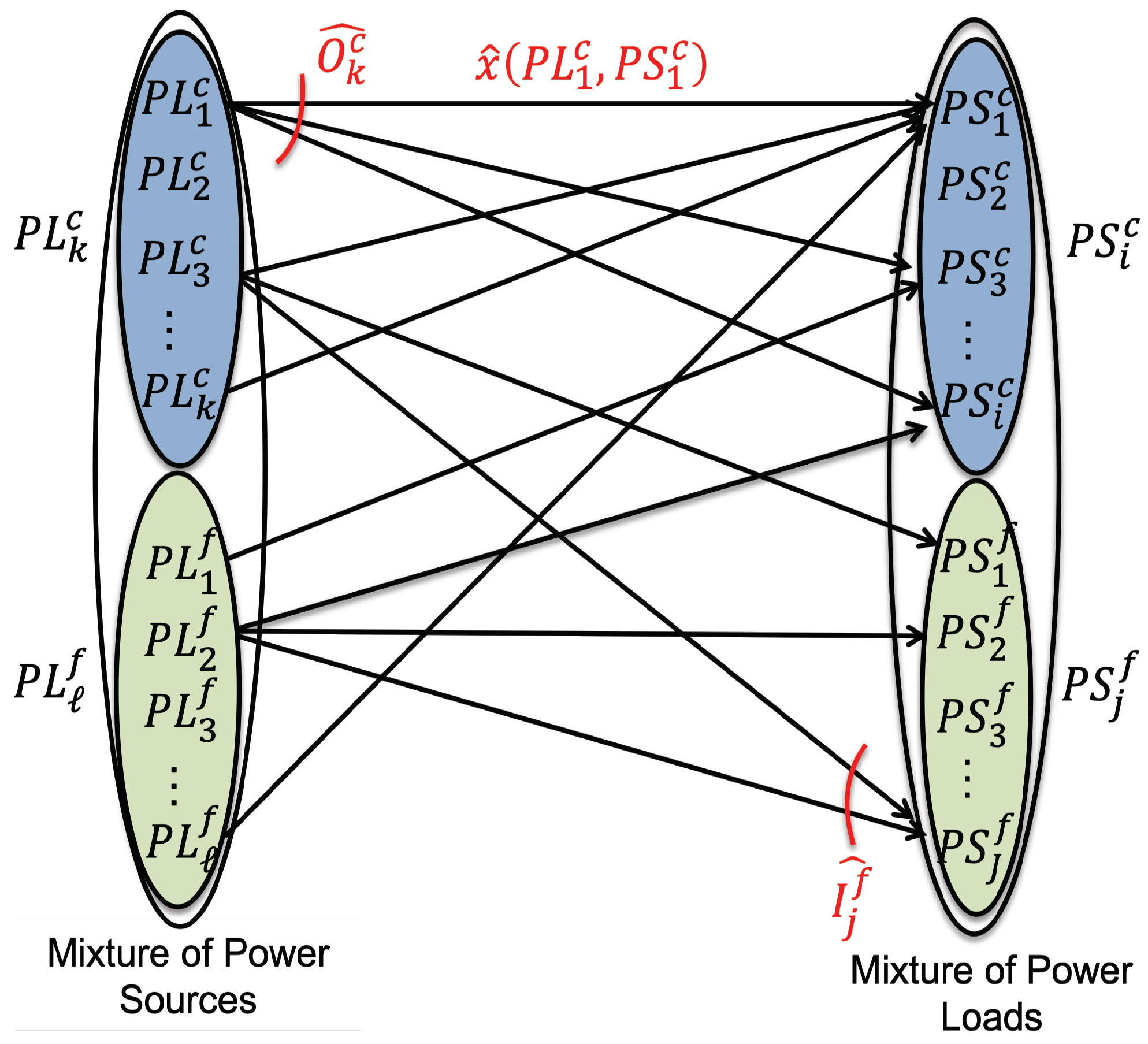
In order to prove the necessity and sufficiency for system condition as given in
2-2 to system condition given in
1-2, at first, we apply interchange of power source devices and load devices (see
Figure 10) so that the relation between
condition 2-2 and
condition 1-2 is mathematically reduced into the relation between
condition 2-1 and
condition 1-1.
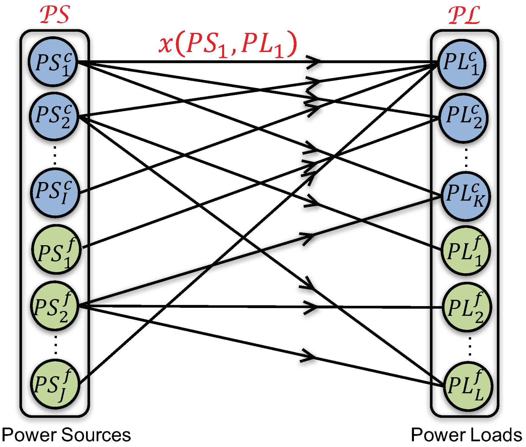
After the interchange of power devices, the representation of power sources of both types i.e., controllable and fluctuating can be shown as where K and L represent the entire group of controllable and fluctuating power sources, respectively. The minimum and maximum power supply limits for controllable power sources can be defined as and for . The power generation limitation for fluctuating power source can be defined as and , respectively, for .
Similarly, the representation of power loads can be replaced as, , where I and J represent the entire group of controllable and fluctuating power loads. The minimum power limitation and maximum power limits for controllable power loads can be defined as and , respectively, for . The consumption limitation can be represented as and for .
According to this exchange of power sources and power loads, we will consider the set of connections , such that if and only if .
After interchange, the condition
1-2 can be seen as condition
1-1 for the transformed system.
In above equation
show the generated power of power sources and
show the power demand of power loads. From the equivalency proof of condition
1-1 to condition
2-1, a power flow assignment exists
, which fulfills the given system conditions for every
and
.
where,
and
show the outgoing power from controllable power sources
and fluctuating power sources
, respectively. The incoming power flows to controllable power loads
and fluctuating power loads
are given as
and
, accordingly.
Subsequently, we return to the original system and consider power flow assignment
x, such that
with outgoing and incoming power flows as,
which shows the equivalency of condition
2-1 to condition
2-2. □


