Appendix A. Calculations for Wire Temperature Gradient
To obtain the partial pressure of cesium, we must produce an experimental curve of thermionic emission versus temperature of the filament. To do so, it is necessary to convert the two observable parameters, the current through the tungsten filament () and the current observed entering collecting conductors () to the temperature of the filament () and to the number of electrons leaving the filament (), respectively.
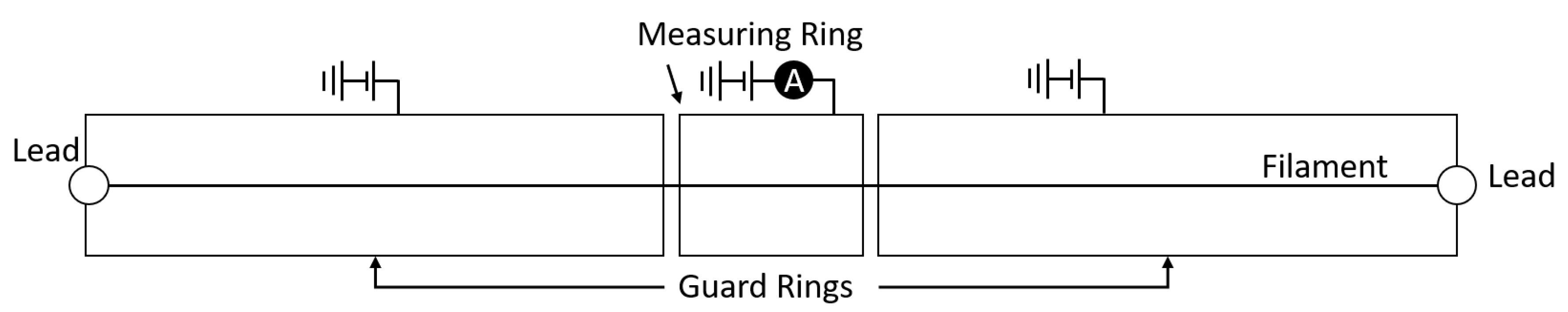
The temperature of the filament is paramount to the characterization of the thermionic current. In their experiments, Taylor and Langmuir made use of guard rings to only measure thermionic electrons from the very center of their filaments so that they may safely assume that its temperature is uniform in that region. However, without using guard rings, and instead measuring electrons from the entire length of the filament, it is necessary to account for the filament’s temperature gradient.
Since the leads conduct heat away from the filament, there is a temperature gradient with a peak at the midpoint. The equation that represents the equilibrium (a steady temperature distribution) for a small part of the filament is:
Where
is the power lost by emission,
is the power from the current through the filament,
is the power conducted in from the hotter end and
is the power conducted out at the colder end (see
Figure A1). Each of these components can be written out as a function of the position in the filament as follows:
where
and
d are the dimensions of the filament, with
l being its long edge,
is the external area of the filament,
is the transverse area of the filament (in our case of a flat filament,
and
, respectively);
is the Stefan–Boltzmann constant,
is the temperature gradient;
i is the current through the filament. Furthermore,
is the resistivity of tungsten as a function of temperature;
is the emissivity of tungsten as a function of temperature; and
is the conductivity of tungsten as a function of temperature. These three tungsten properties were all fitted to 4th or 5th order polynomials as a function of T.
Figure A1.
Power transport scheme for a small piece of the filament, the different pieces are numbered as they are used in Equations (
A2)–(
A9). The Black arrows indicate power into the filament piece, and the grey arrows indicate power out.
is the power piece 3 conducts from piece 4 into the center piece, and
is the power piece 2 that conducts from the center piece to piece 1.
Note that Equations (
A4) and (
A5) can be re-written as a function of the first derivative of
at
and
, respectively:
Substituting Equations (
A2), (
A3), (
A6), and (
A7) back into Equation (
A1), we have:
which can also be re-written as a function of the second derivative of
:
This is a second order differential equation that can be solved numerically for
with two boundary conditions. We assume knowledge of the temperature of the ends of the filament, which is valid if the leads they are connected to are heat-sunk to the manifold. The manifold temperature is measurable from the outside. Furthermore, given that at high temperatures
is small, we assume that, for the very center of the wire, where it is hottest, Equation (
A1) has negligible conduction summands, and thus we can solve for the temperature at the midpoint given a current. Therefore, we have both
and
as boundary conditions. Solving for
, we get, for any current, a temperature gradient in the filament.
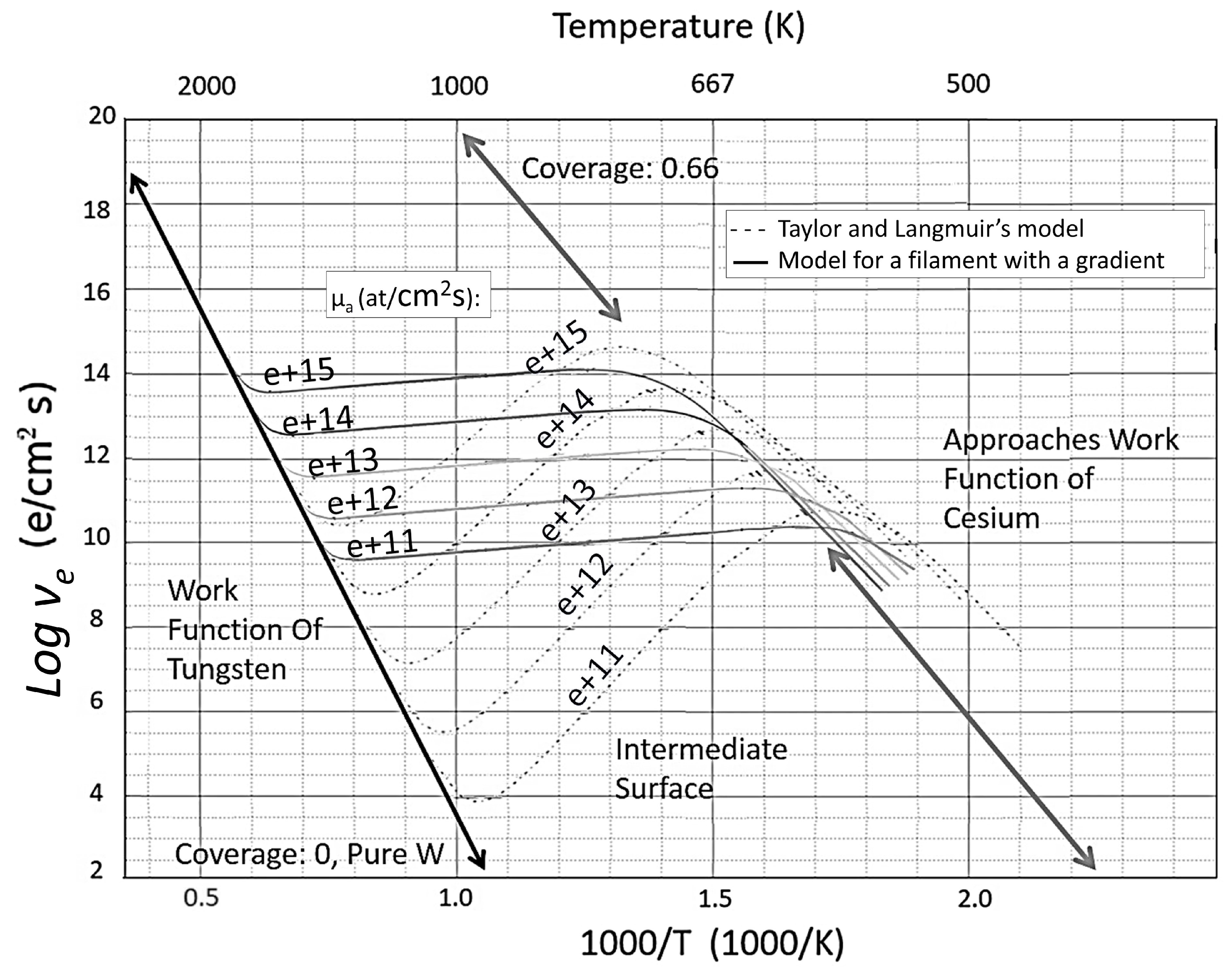
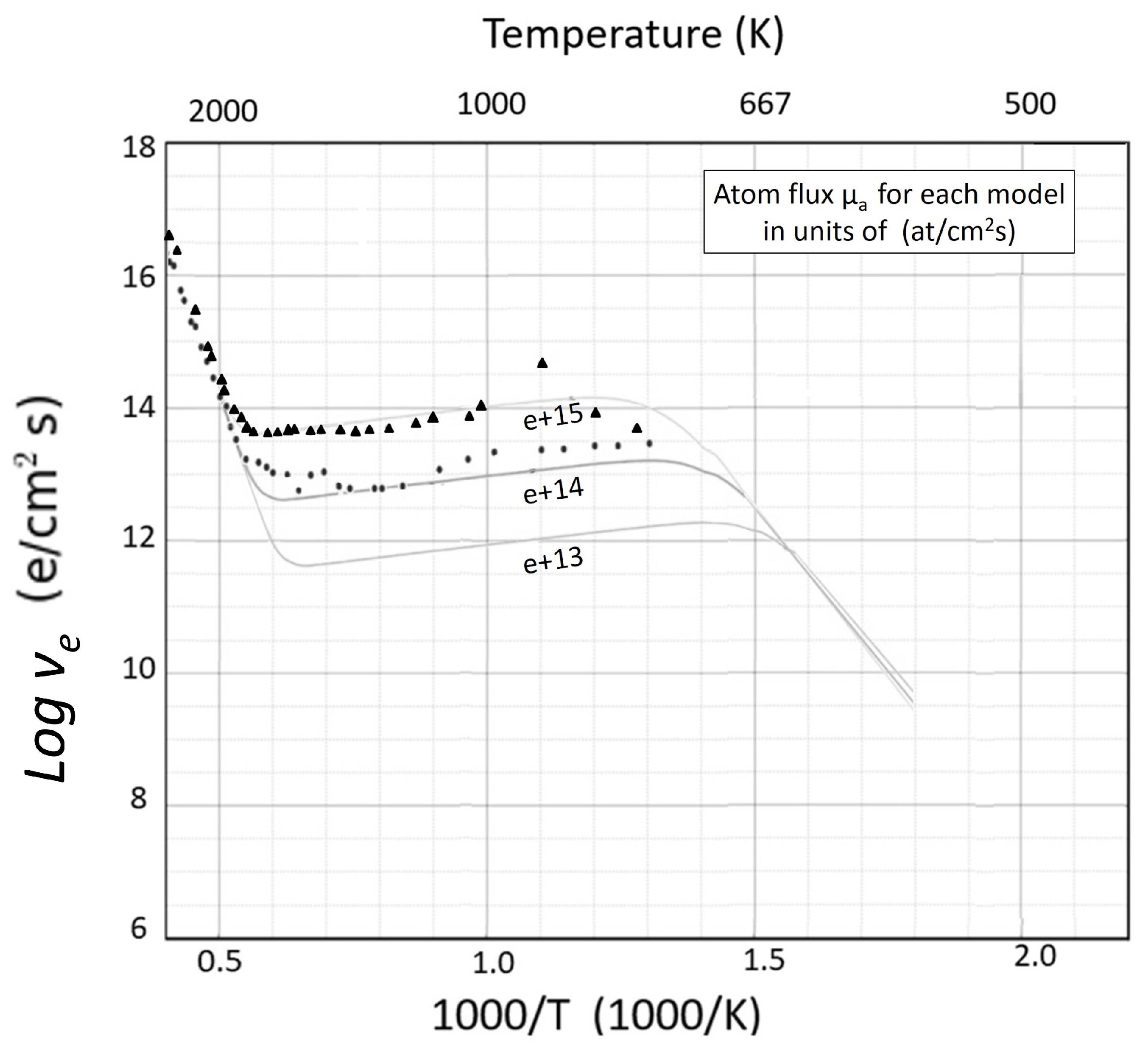
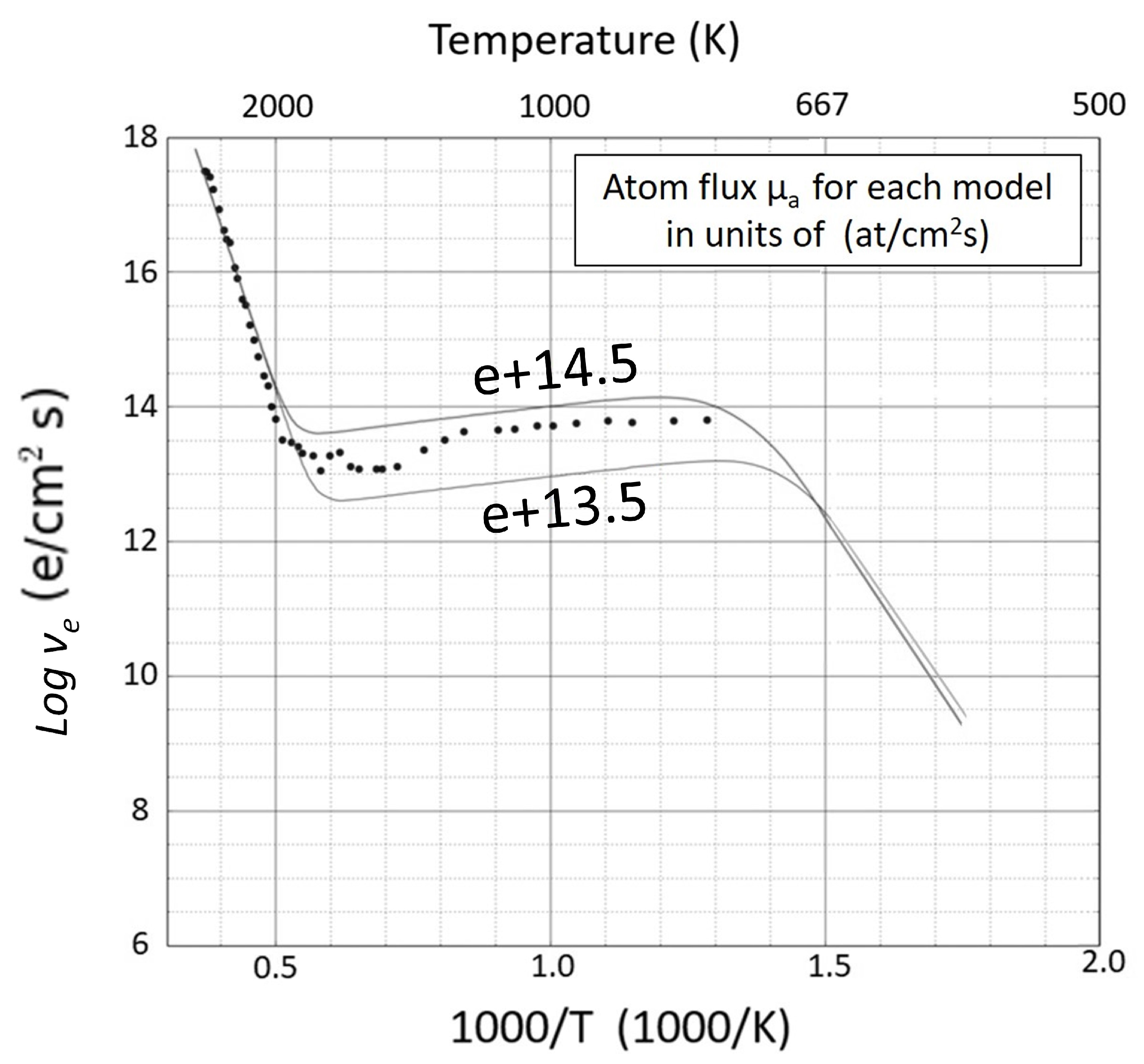
Once we have
, we can perform a numerical integration of how many thermionic electrons will be emitted by different parts of the filament based on Taylor and Langmuir‘s experimentally determined curve. We do this to calculate the predicted thermionic emission from a filament with non uniform temperatures, and we can generate a curve analogous to Taylor and Langmuir‘s but for a filament with a temperature gradient instead of a uniformly heated filament (See dotted lines in
Figure 1).
Appendix B. Operation Precautions
A measurement with the gauge has been described above. However, to obtain reproducible results, certain precautions must be taken.
Taylor and Langmuir recommend that before any measurement is done the filament undergoes what they call an aging process. This involves leaving the filament heated at 2400 K for 10 h, then at 2600 K for an hour, and finally concludes with a few brief flashes at 2900 K. Prior to such aging, neither we nor Taylor and Langmuir could obtain reproducible results. Furthermore, we have determined that brief flashes to about 2500 K before any measurement generate more reproducible results as well.
It is also necessary that the measurement not interfere appreciably with the temperature of the source of cesium. The filament heats up to high temperatures during the measurement (up to 2500 K) and, if the cesium source temperature changes mid-measurement, so will the pressure of cesium vapor. A fast measurement can solve this issue, as well as placing the source far away from the filament or using a thinner filament.
Leakage currents between the charged plates and either ground or the filament terminals increase the background in the measurement of the currents collected from the plates. We attribute this leakage current to condensed cesium on the ceramic tile connecting the ends of the filament, the plates, and the manifold together.
There are two ways leakage currents interfere with the measurements. It makes it so that the signal measured across the series resistor does not only come from collected thermionic electrons, but also from ground electrons that arrive from leakage conductive paths. Furthermore, as one changes the temperature of the conductive paths, cesium evaporates or condenses, thus changing the resistance of the leakage pathways. This means that there is not a simple static current background one might subtract from the measured signal.
It is possible to deal with such currents. By applying high voltages to the circuit elements, any conductive cesium paths to ground will heat up and the cesium will evaporate off the surfaces. For the charged plates, half an hour at 300 V took a 10 k short to up to tens of M. Such voltages required the use of high-voltage power source. Another effective counter to leakage currents was to keep the gauge much hotter than the source to avoid creating sites prone to cesium deposition. When source and manifold were left at the about the same temperature, all of the circuit elements were connected to each other and to the ground by resistances under one k. When the manifold was left at four times the temperature of the source, however, resistances went up to hundreds of k.


