A Parameter Refinement Method for Ptychography Based on Deep Learning Concepts

Abstract

X-ray ptychography is an advanced computational microscopy technique, which is delivering exceptionally detailed quantitative imaging of biological and nanotechnology specimens, which can be used for high-precision X-ray measurements. However, coarse parametrisation in propagation distance, position errors and partial coherence frequently threaten the experimental viability. In this work, we formally introduce these actors, solving the whole reconstruction as an optimisation problem. A modern deep learning framework was used to autonomously correct the setup incoherences, thus improving the quality of a ptychography reconstruction. Automatic procedures are indeed crucial to reduce the time for a reliable analysis, which has a significant impact on all the fields that use this kind of microscopy. We implemented our algorithm in our software framework, SciComPty, releasing it as open-source. We tested our system on both synthetic datasets, as well as on real data acquired at the TwinMic beamline of the Elettra synchrotron facility.

1. Introduction

In the last decade, computational microscopy methods based on phase retrieval [1] have been extensively used to investigate the microscopic nature of thin, noncrystalline materials. In particular, quantitative information is provided by ptychography [2,3], which combines lateral scanning with Coherent Diffraction Imaging (CDI) methods [4,5]. Similar to Computed Tomography (CT) [6,7], the technique tries to solve an inverse problem, as the object is reconstructed from its effects impinged on the incident beam. The result is a high-detail absorption and quantitative phase image of large specimens [8]. In a transmission setup (e.g., in a synchrotron beamline microscope [9,10]), this reconstructed object is a complex-valued 2D transmission function $O(x,y)$, which describes the absorption and scattering behaviour [11] of the sample.

1.1. Iterative Phase Retrieval

Typically, an iterative phase retrieval procedure [1] is employed to find a solution for $O(x,y)$ [3]: an a priori image formation model is used to simulate the experiment, by producing synthetic quantities (Figure 1), which depend on the current estimate of all the latent variables, e.g., $O(x,y)$, and the model parameters; it is the comparison (loss function) between simulated and measured quantities that guides the solution, as the current estimate is iteratively updated (Figure 2) to minimise the error. In CDI/ptychography, the quantities of interest are diffraction patterns (Figure 1).

1.2. The Parameter Problem

Ptychography is extremely sensitive to a coarse parameter estimation [12,13], and this may result in a severely degraded reconstruction: a long trial and error procedure is typically employed to manually refine these quantities, looking for an output with fewer artefacts. On the contrary, framing the reconstruction as a gradient-based optimisation process (Figure 2), the loss function can be written with an explicit dependency on the model parameters, for which an update function can be calculated. As the model complexity increases, the gradient expressions become progressively more difficult to calculate, and indeed, Automatic Differentiation (AD) methods (also referred to as “autograd”) [14,15] applied to ptychography are recently receiving much attention as an effective way to design complex algorithms [16,17,18]. However, being based on fixed parameters, the presented reconstruction algorithms can eventually become fragile (except for [18]), requiring some interventions.

1.3. Proposed Solution

In the present work, we describe an AD-based ptychography reconstruction algorithm that takes into account many setup parameters within the same optimisation problem. The procedure was solved entirely within an AD environment. This was made possible as a loss function was derived by explicitly taking into account all the setup parameters, which were added to the optimisation pool for a joint regression/reconstruction. It has to be noted that also the probe positions were refined in this way, without using an expensive Fourier-transform-based approach. Indeed, a deep-learning-inspired strategy was employed, rooted in the spatial transformer network literature [19]. The software has been released as open-source [20].

1.4. Manuscript Organisation

This paper is organised as follows: in Section 2, we provide a brief introduction to the ptychography forward model, defining the major flaws we wanted to correct, as well as a brief description of the autograd technology. In Section 3, our computational methodology is described, introducing the designed loss function and the spatial transform components. In Section 4, we present our main results, while Section 5 concludes the paper.

2. Background

In ptychography [3] (Figure 3), an extended object is placed onto a sample stage and is illuminated with a conic beam of monochromatic and coherent light. The radiation illuminates a limited region of the specimen (see the dotted circles in Figure 3), and a diffraction pattern is recorded by a detector placed at some distance $z_{sd}=z_d-z_s$ (see Figure 3). To reconstruct the object, both the set of J recorded diffraction patterns $I_j$ with $j\in [1\dots J]$ and the J$(x_j,y_j)$ positions are required. Each jth acquisition can be considered independent of the others. By illuminating adjacent areas with a high overlap factor, diversity is introduced to the acquisition, thus creating a robust set of constraints, which greatly improve the convergence of the phase retrieval procedure [3]. Diversity is what helps the optimisation problem regress the setup parameters.

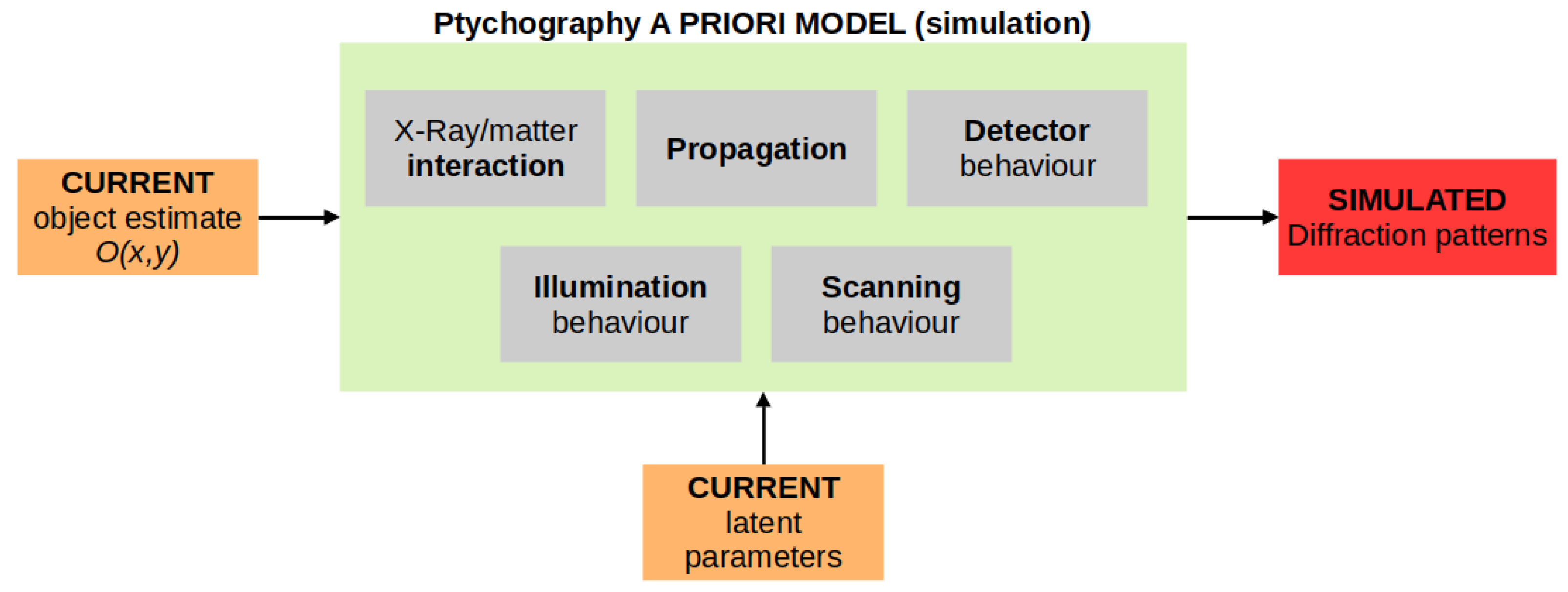
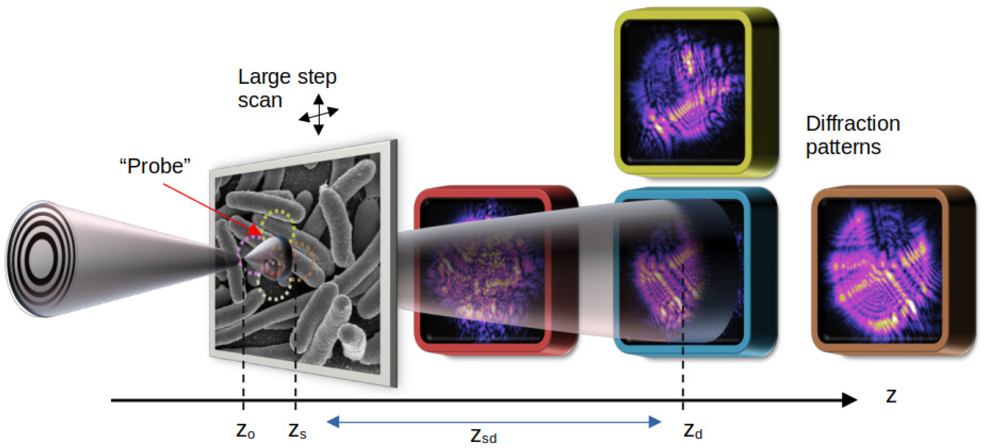
2.1. Ptychography Model

The image formation model schematised in Figure 1 can be described more formally by the following expression:

$$I_j(x,y;z_d)={\left|D_{z_d-z_s}\{P(x,y;z_s)·O(x_j,y_j;z_s)\}\right|}^2,$$

(1)

where $P(x,y;z_s)$ is the 2D illumination on the sample plane ($z=z_s$), typically referred to as the “probe”; $O(x_j,y_j;z_s)$ is the 2D transmission function of the sample in the local reference system $(x_j,y_j)$, centred at the known jth scan position; $D_{z_d-z_s}$ is an operator that describes the observation of the pattern at a known distance $z_d-z_s$.

Knowing the illumination on a region of the object is crucial for the factorisation of the exit wave ${\mathsf{\Psi }}_s(x,y;z_s)$:

$${\mathsf{\Psi }}_s(x,y;z_s)=P(x,y;z_s)·O(x_j,y_j;z_d).$$

(2)

In a modern ptychography reconstruction, $P(x,y)$ is automatically found thanks to the diversity in the dataset [3,21,22], and the “probe retrieval” procedure has been extended also to the case of a partial coherence [3,23,24,25,26]. Indeed, in order to take into account the independent propagation of M mutually incoherent probes, Equation (1) is modified in the following manner:

$$I_j(x,y;z_d)=\sum _{p=1}^M{\left|D_{z_d-z_s}\{P_p(x,y;z_s)·O(x_j,y_j;z_s)\}\right|}^2,$$

(3)

where the exit wave produced by the modulation of each $P_p(x,z;z_s)$ mode is summed in intensity on the observation plane $z_d$.

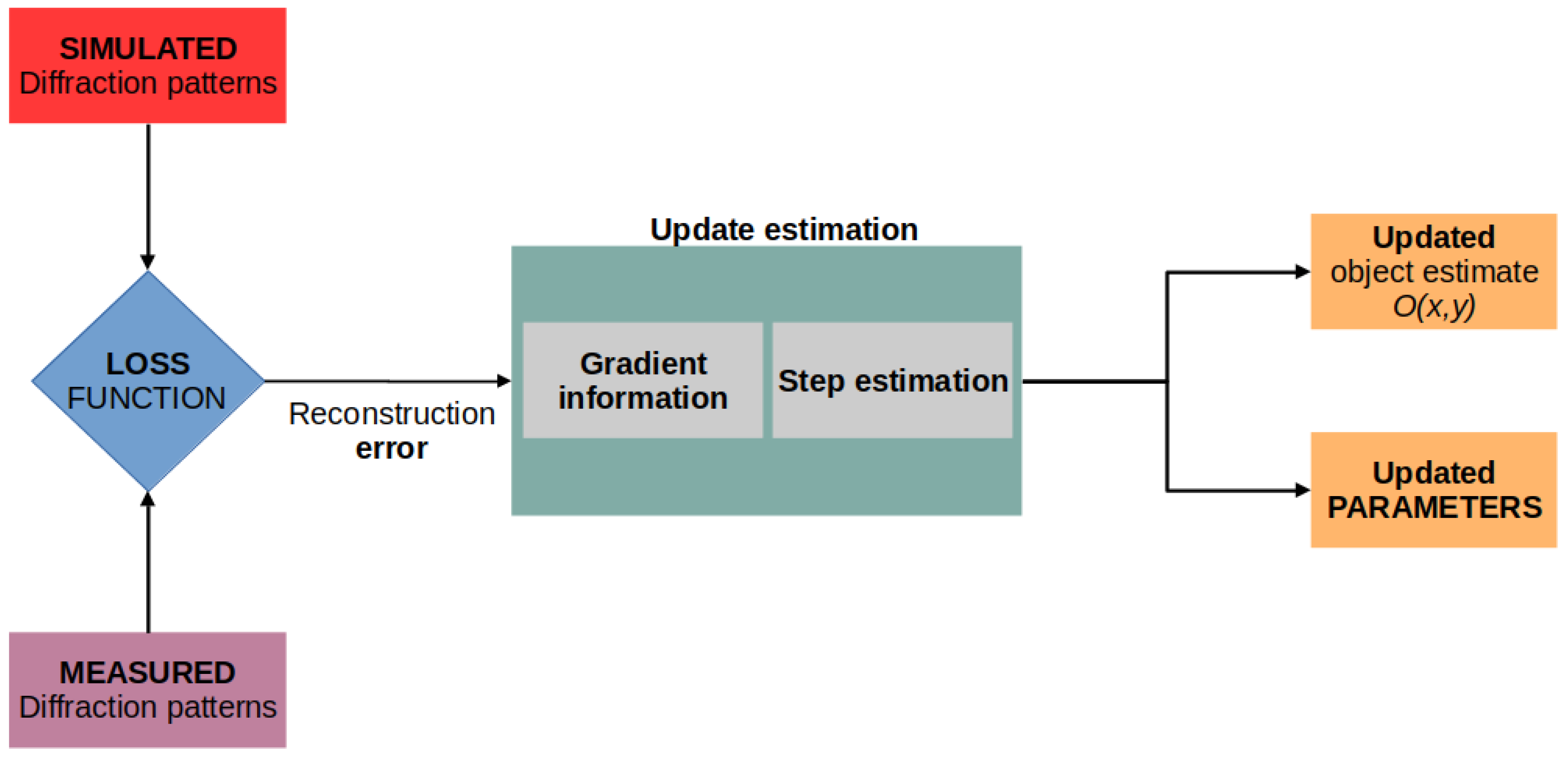
2.2. Parameter Refinement

We can denote as the “setup incoherences” all the deviations of a real setup from the a priori model defined in Equation (1). Even if in the literature, many solutions have been proposed, in most cases, the problems are typically tackled independently. Partial coherence and mixed-state ptychography have been extensively reviewed (e.g., in [3,27,28]); the same is valid for the position refinement problem [29,30,31,32,33,34,35], with methods that are quite similar to what is performed in, e.g., super-resolution imaging [36] or CT [37]. To understand the importance of positions for ptychography, Figure 4 illustrates a slightly exaggerated condition: note that the entire object computational box changes format, and this is detrimental, especially from the implementation point of view.

Much more scarce is the literature on axial correction: in [13], an evolutionary algorithm was used to cope with the uncertainty of the source-to-sample distance in electron ptychography. In [38], the authors proposed using a position refinement scheme also to correct for the axial parameters, as the latter is responsible for modifying the distances between adjacent probes, while in a work published in January 2021, the authors of [39] used an autograd environment to directly infer the propagation distance.

In an even more recent work (March 2021), the authors in [18] proposed also a unifying approach to parameter refinement similar to the one used in our manuscript: we genuinely only became aware of these two references while writing the final version of this manuscript. It is undoubted that the automatic differentiation methods (Section 2.3) are becoming of interest for computational imaging techniques such as ptychography, and many research teams are approaching the methods as they represent the future of the technique.

Figure 5 shows the effect of the wrong propagation distance on the probe retrieval procedure: in Panel A, speckle-like patterns typically appear; position errors produce instead a typical dotted artefact. An incorrectly retrieved probe $P(x,y)$ will produce a severely wrong object reconstruction $O(x,y)$.

2.3. Automatic Differentiation

An unconstrained optimisation problem aims at minimising a real-valued loss function $f\left(\mathbf{x}\right)$ of N variables. This problem can be formally expressed by the following way:

$$\tilde{\mathbf{x}}=\underset{\mathbf{x}}{argmin}f\left(\mathbf{x}\right),$$

(4)

where $\tilde{\mathbf{x}}$ is the sought N-vector solution. One of the common methods to iteratively minimise the function $f\left(\mathbf{x}\right)$ is the gradient descent procedure, which relies on the gradient of the loss function to define an update step:

$${\mathbf{x}}_{k+1}={\mathbf{x}}_k-\alpha {\nabla }_{\mathbf{x}}{f\left(\mathbf{x}\right)|}_{\mathbf{x}={\mathbf{x}}_k}$$

(5)

which will provide a new vector estimate ${\mathbf{x}}_{k+1}$ from the previous estimate ${\mathbf{x}}_k$, which at convergence will be equal to $\tilde{\mathbf{x}}$. The handmade symbolic computation of ${\nabla }_{\mathbf{x}}f\left(\mathbf{x}\right)$ becomes increasingly tedious and error-prone as the complexity of the expression increases. Numerical differentiation automatically provides an estimate of the point derivative of a function by exploiting the central difference scheme, but while this method is particularly effective for a few dimensions, it becomes progressively slow as N increases. On the other side, a Computer Algebra System (CAS) generates a symbolic expression through symbolic computation, but often, the output results in expression swell. Automatic differentiation [40,41,42] is a way to provide an accurate gradient calculated at a point, thus lying in between numerical differentiation and handmade calculation. In one of the currently used methods to automatically compute the gradients [43], when a mathematical expression is evaluated, each temporary result constitutes a node in a computational acyclic graph that records the story of the expression, from the input variables to the generated result. The gradient is simply calculated following the graph backwards (backward mode differentiation [42]), from the results to the input variables, only applying the chain rule to the gradient of each nuclear differentiable operator [40].

3. Computational Methodology

The ptychography forward model is defined in terms of a complex probe vector $\mathbf{P}\in {\mathit{C}}^K$ interacting with a complex object transmission function, which can also be arranged as a vector $\mathbf{O}\in {\mathit{C}}^D$.

3.1. Loss Function

Loss functions are typically designed around simple dissimilarity metrics such as quadratic norms, which can be real functions of a complex variable. As represented in Figure 2, the loss function takes into account the simulated ($\widetilde{I_j}$) and real ($I_j$) quantities of the same type (diffraction patterns). When all the conditions defined in Section 2 hold, a loss function $\mathcal{L}$ for all the $j\in [1\dots J]$ diffraction patterns and positions in the dataset can be written as a data fidelity term:

$$\mathcal{L}(\mathbf{P},\mathbf{O},z)=\sum _{j=1}^J{∥\widetilde{I_j}(\mathbf{P},\mathbf{O},z)-I_j∥}^2.$$

(6)

As can be seen, Equation (6) is a function of the $2K+2D+1$ real variables, which when stacked up, constitute the optimisation vector pool. The simulated diffraction pattern $\widetilde{I_j}$ relative to the current jth computational box is calculated by Equation (1) or by its extension to a multimode illumination (Equation (3)). The square root of the recorded data can be computed once for all the diffractions to fasten the implementation. $D_z$ is the angular spectrum propagator [44] defined by the expression:

$${\mathsf{\Psi }}_d(x,y;z_d)={\mathcal{F}}^{-1}\{\mathcal{F}\left\{{\mathsf{\Psi }}_s(x,y;z_s)\right\}·\mathcal{F}\left\{h(x,y,z)\right\}\},$$

(7)

which relates the input field ${\mathsf{\Psi }}_s(x,y;z_s)$ (defined in Equation (2)) to the output field at the detector plane ${\mathsf{\Psi }}_d(x,y;z_d)$. Fixing the wavelength $\lambda$ of the incident radiation, the 2D Fourier transform of the propagation filter h is defined by [44]:

$$\mathcal{F}\left\{h(x,y,z)\right\}=H(f_x,f_y,z)=e^{jkz·\sqrt{1-{\left(\lambda f_x\right)}^2-{\left(\lambda f_x\right)}^2}}.$$

(8)

3.2. Complex-Valued AD

Current DL autograd tools are not conceived of to work with complex numbers, so a basic complex library needs to be written; the natural way to introduce them is to just add an extra dimension to each 2D tensor and incorporate the real and the imaginary part in the same object, basically duplicating the number of actual variables. The automatic backward operation is completely acceptable for this kind of custom-made data type, and the resulting gradient is simply:

$$gradf\left(\mathbf{x}\right)=2{\nabla }_x^{\ast }f\left(\mathbf{x}\right)=\frac{\partial f}{\partial {\mathbf{x}}^{\ast }}=(\frac{\partial f}{\partial \mathbf{a}}+j\frac{\partial f}{\partial \mathbf{b}})$$

(9)

where $\mathbf{x}=\mathbf{a}+j\mathbf{b}$. The actual gradient is represented in the same complex data type of the variables, made of a real and an imaginary part. As can be seen in Equation (9), the result of the automatic differentiation can be written in the Wirtinger formalism [45], just as the derivative with respect to the conjugate of the differentiation variable (except for the constant), which is the typical gradient expression exploited for functions of complex variables.

3.3. Regularisation

To increase the quality of the reconstruction, the data fidelity term in a loss function is usually paired with a regularisation term (the method of Lagrange multipliers), whose role is to penalise ad hoc solutions in the parameter space: a pixel value ought to fit the physical nature of the model beneath, without only accommodating the dissimilarity measure; this translates into a mere energy-conservation constraint. Other regularisation methods can be employed, especially the one based on priors on the image frequencies; however, they can be more difficult to tune and require a different forward model. Different from other works (e.g., [17,18]), in this work, especially for $\mathbf{O}$ and $\mathbf{P}$, we decided to use energy-based regularisation, paired only with a large penalisation of quantities out of the desired range. In this way, we practically constrained the minimisation even if a nonconstrained optimisation framework was used.

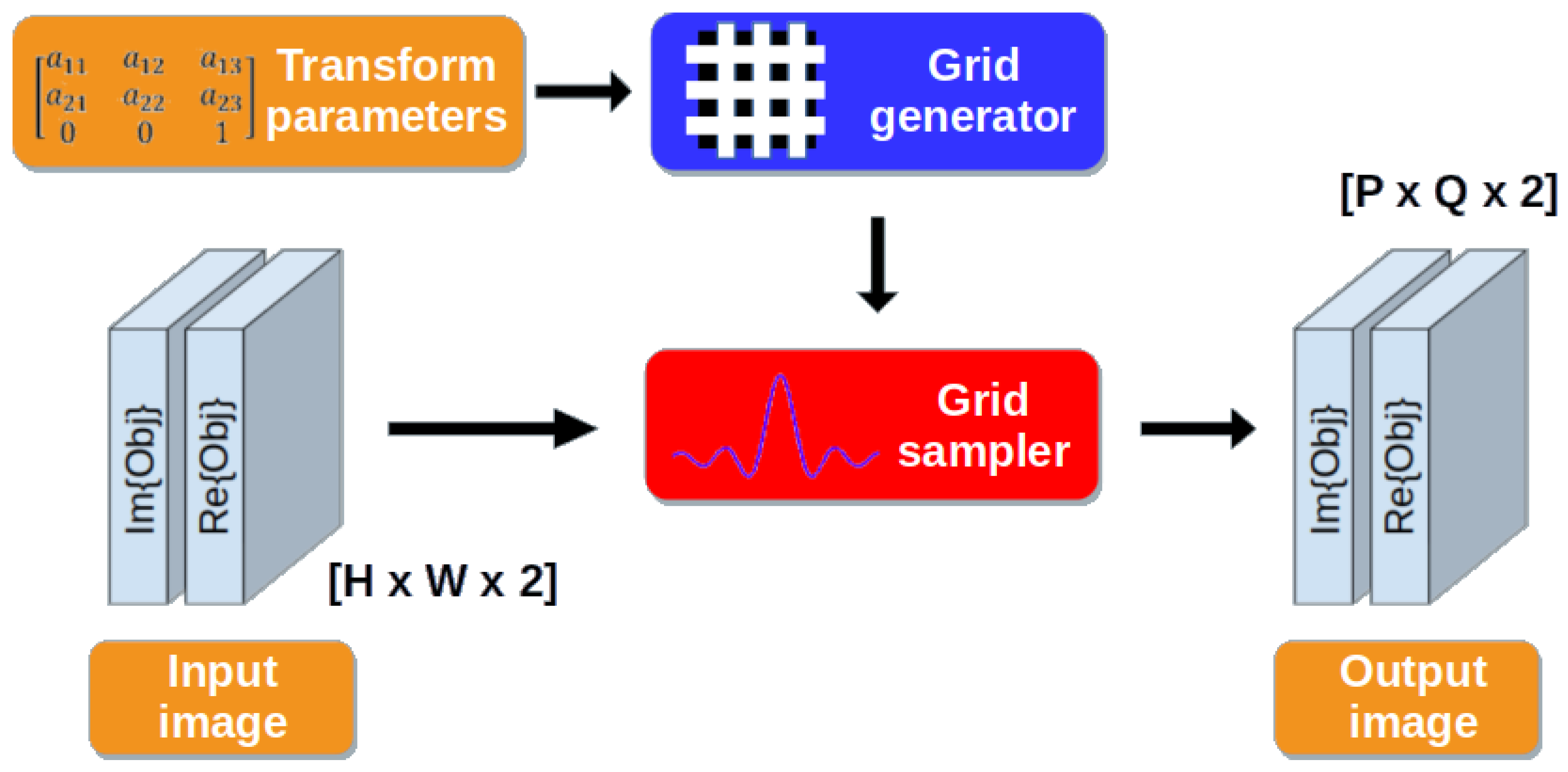
3.4. Spatial Transform Layer

If as seen in Equations (6) and (7), writing a mathematical expression in the parameters $\mathbf{O}$, $\mathbf{P}$ and z directly permits the gradient generation, the same does not hold for the spatial shift correction defined on a discrete sampling grid. Indeed, in the typical ptychography reconstruction algorithm, the computational box for a given jth position is defined by exploiting a simple crop operator on a 2D tensor. While this method is simple and computationally fast (pointer arithmetics), it is not differentiable, as integer differentiation is nonsense. In this work, an approach borrowed from the DL community was then explored.

Convolutional neural networks are not invariant to geometric transforms applied to their input. To cope with this problem, a spatial transform layer [19] is introduced; the new learnable model is trained by inferring the spatial transformation that, applied to the input feature map, maximises the task metric. This approach greatly improves classification and recognition performances (e.g., in face recognition [46]).

In this work, instead, the parameters of the affine transform were directly learned as the position refinement coefficients, which minimise the objective function (Equation (6)) during the reconstruction. To do so, two components were used (Figure 6): (I) a grid generator and (II) a grid sampler. The first element transforms a regular input sampling grid ${(x_i,y_i)}^T$ into an output coordinates grid ${(x_o,y_o)}^T$, by applying an affine transform to the former; this mapping (Equation (10)) is fully defined by six degrees of freedom, but as concerns rigid translation, only the last column ${(t_x,t_y)}^T$ is optimised. The scaling factors ${(s_x,s_y)}^T$ are thus constants used to crop the central region.

$${\left(\begin{array}{c}{x}_o\\ y_o\end{array}\right)}_j={\left(\begin{array}{ccc}{s}_x& 0& t_x\\ 0& s_y& t_y\end{array}\right)}_j{\left(\begin{array}{c}{x}_i\\ y_i\end{array}\right)}_j$$

(10)

Then, for each jth diffraction pattern and each jth shift-vector ${(t_x,t_y)}^T$, the jth output grid ${(x_o,y_o)}^T$ is generated. From the latter, the grid sampler thus outputs a warped version of the object. Following the formalism introduced in [19], the cropped portion of the object $V_j$ is generated from the entire object U by:

$$V_j=\sum _{h=1}^H\sum _{w=1}^W{U}_{w,h}·K(w-x_j,h-y_j)$$

(11)

A well-performed sampling (with an antialiasing filter) adds a regularisation term that can help during the optimisation. The bilinear sampling exploits a triangular (separable) kernel K, defined in Equation (12), which does not present dangerous overshooting artefacts:

$$K(w-x,h-y)=K_1(w-x)·K_1(h-y)$$

(12)

where:

$$K_1\left(t\right)=max(0,1-|t\left|\right).$$

(13)

Figure 6 shows the structure of the proposed approach, applied to the ptychography framework. The same spatial transform is enforced on the two channels of the tensor that represent the real and imaginary parts of the cropped region of the object. Within this setup, gradient propagation is possible because derivative expressions can be calculated with respect to both the affine grid and the output pixel values [19].

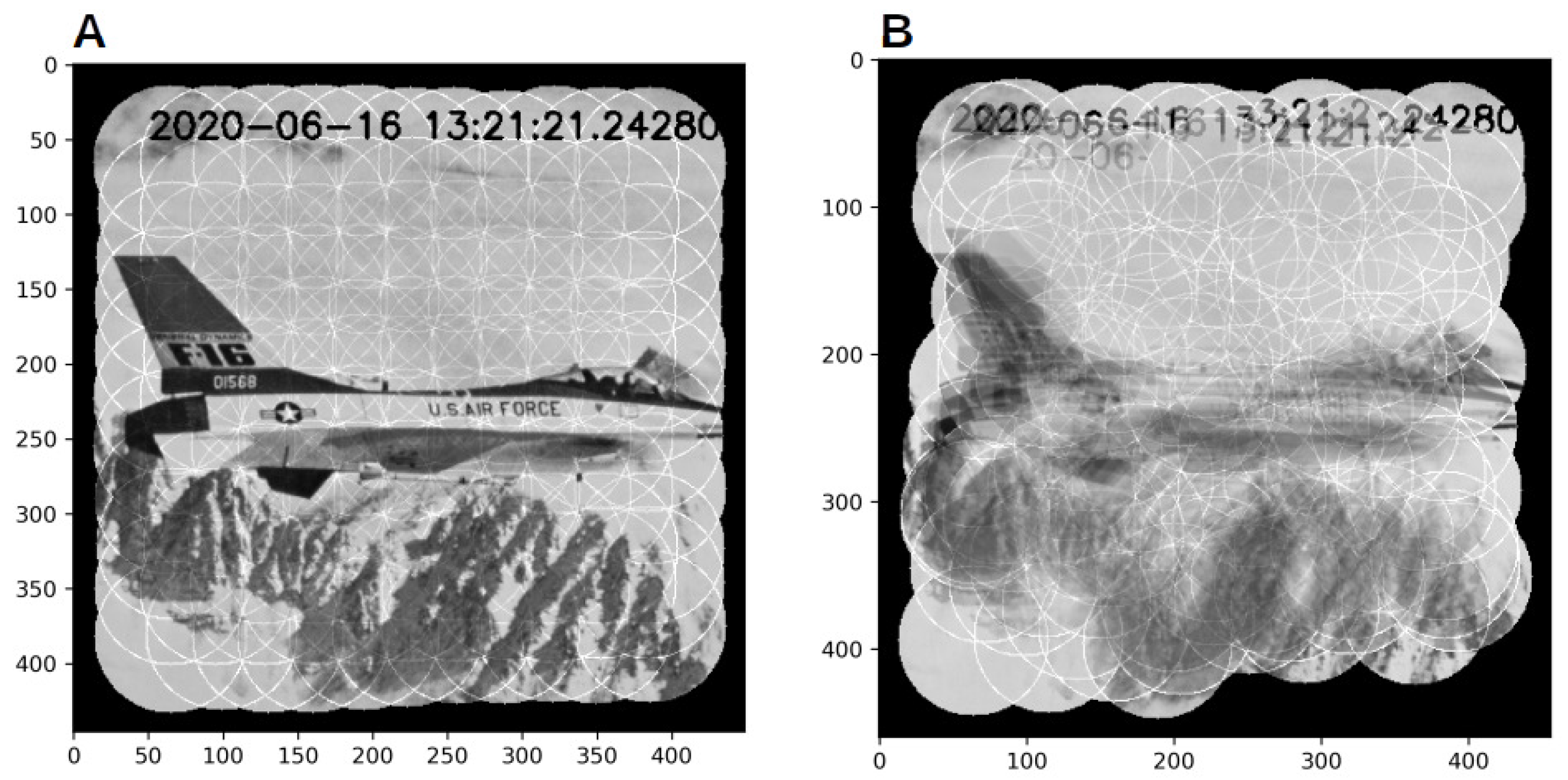
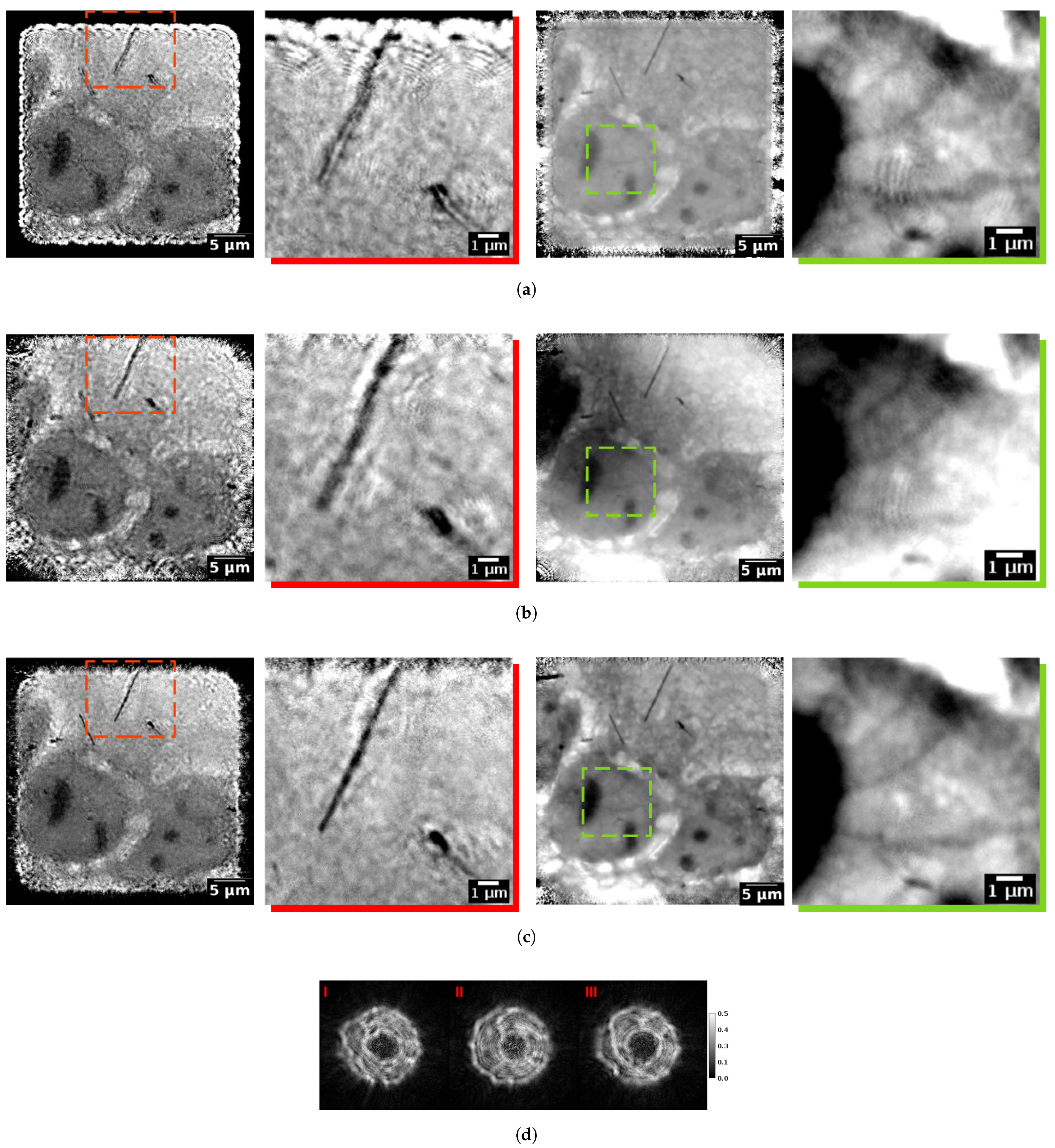
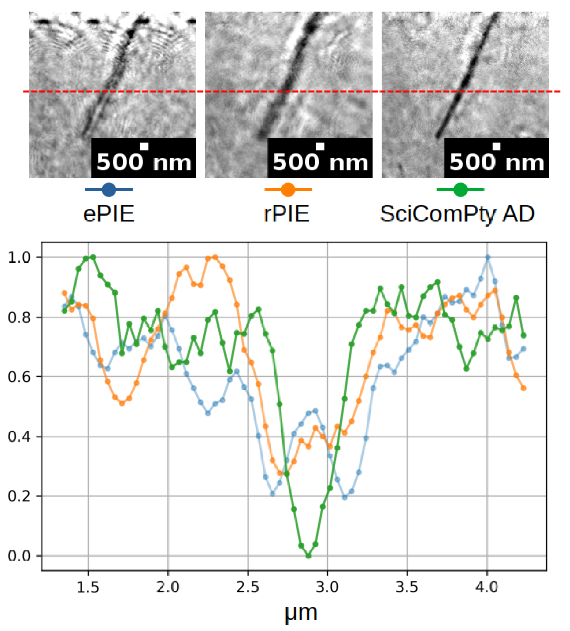
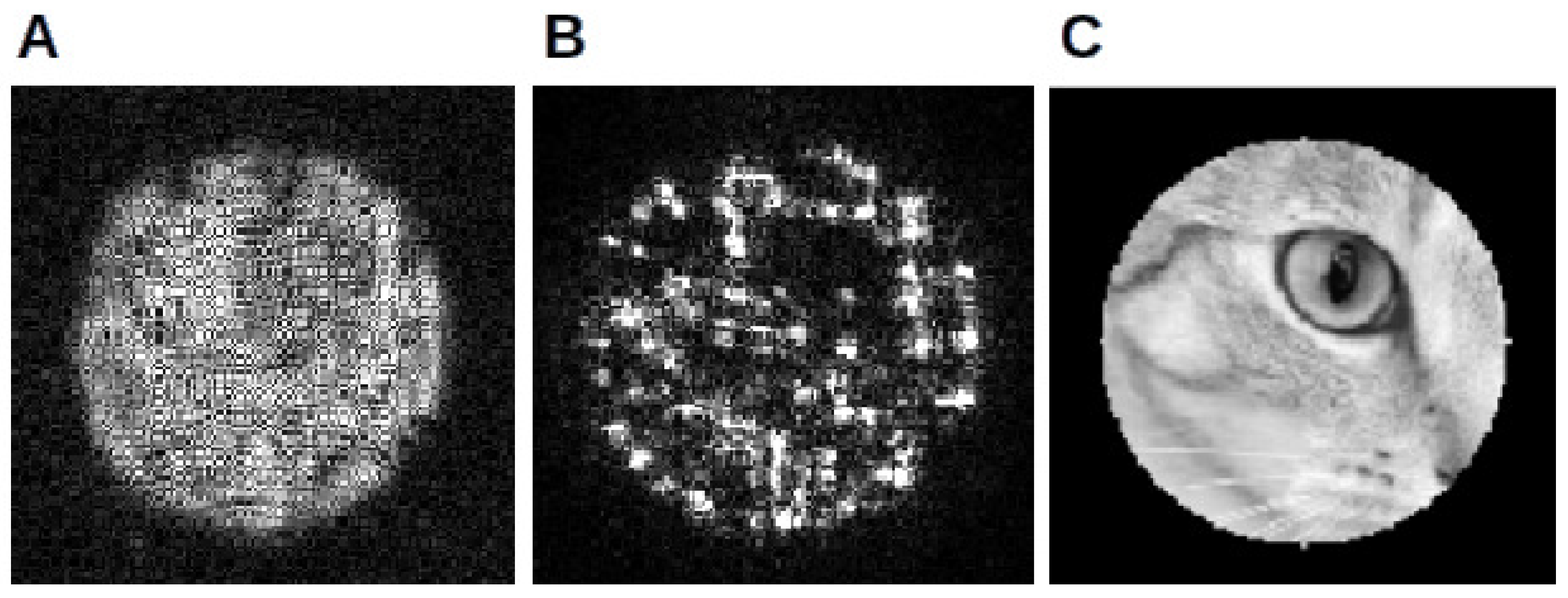
4. Results and Discussion

In this section, reconstructions obtained from a soft X-ray experiment are presented. Additional details on the performance analysis for many synthetic datasets can be found instead in the Supplementary Materials of this publication. The reconstruction obtained through the proposed method is confronted with the output of the EPIE [22] and RPIE [47] algorithms. The virtual propagation distance of $0.037$ mm was chosen by reconstructing at many z and selecting the best reconstruction. All the computational experiments were written on PyTorch 1.2 [43] and executed on a computer equipped with an Intel Xeon (R) E3-1245 v5 CPU running at 3.50 GHz. The entire code was implemented on a GPU (Nvidia Quadro P2000), which is essential for this heavy-duty computational imaging.

The imaging experiment was performed at the TwinMic spectromicroscopy beamline [9,10] at the Elettra synchrotron facility. TwinMic can operate in three imaging modalities: (I) STXM; (II) full-field TXM/CDI; (III) scanning CDI (ptychography). Clearly, the latter (the one used for this work) is obtained by combining the optic setup of the second modality and the control of the sample stage from the first one.

Similar to other ptychography experiments performed at the beamline (e.g., [10,48]), X-ray data were collected using a 1020 eV X-ray synchrotron beam [9] focused with a 600 $\mathsf{\mu }$$\mathrm{m}$ diameter Fresnel Zone Plate (FZP) with an outer zone width of 50 $\mathrm{n}$$\mathrm{m}$. The zone plate was placed approximately at 2 m downstream a 25 $\mathsf{\mu }$$\mathrm{m}$ aperture that defines a secondary source. This is crucial to increase the beam coherence, at the expenses of brightness. A Peltier-cooled Charge-Coupled Device (CCD) detector (Princeton MT-MTE) with 1300 × 1340 $20 \mathsf{\mu }\mathrm{m}\times 20$ $\mathsf{\mu }$$\mathrm{m}$ px${}^2$ was placed roughly 72 cm downstream of the FZP. According to the Abbe theory [48], the limit of the resolution for coherent illumination is $\Gamma =0.82\lambda /NA$ = 50 nm. The resolution in Fresnel CDI is a function of the experimental geometry [49], namely the distance from the focal point of the FZP to the detector and the physical size of the detector itself, rather than the focusing optics.

From the ptychography configuration point of view, the situation is similar to the one presented in [50], where a point source (obtained by idealising the focus of an FZP through an order sorting aperture) illuminates the sample. Following the approach of [50], during the data analysis, the beam was parallelised by using the Fresnel scaling theorem [44]. In the following experiment, as pointed out in Section 2, the sample was considered sufficiently thin [21,51] to be modelled by a multiplicative complex transmission function O defined by the expression:

$$O\left(\mathbf{r}\right)=e^{j\frac{2\pi }{\lambda }[n\left(\mathbf{r}\right)-1]t\left(\mathbf{r}\right))}=e^{j\frac{2\pi }{\lambda }t\left(\mathbf{r}\right)[-\delta \left(\mathbf{r}\right)+j\beta \left(\mathbf{r}\right)]}$$

(14)

where $\mathbf{r}$ is the planar coordinate on the sample plane, $n\left(\mathbf{r}\right)$ is the complex refraction index and $t\left(\mathbf{r}\right)$ a real $R^2\mapsto R^1$ function defining the local thickness. From the reconstruction-inferred $O\left(\mathbf{r}\right)$ (the objective of the reconstruction), the magnitude map corresponds to:

$$ln\left|O\left(\mathbf{r}\right)\right|=ln\sqrt{I\left(\mathbf{r}\right)}=ln\sqrt{I_o\left(\mathbf{r}\right)}-\frac{2\pi }{\lambda }\beta \left(\mathbf{r}\right)·t\left(\mathbf{r}\right)$$

(15)

where $I_o$ is the flat field intensity and I the sample intensity. The phase map instead corresponds to:

$$\arg \left\{O\left(\mathbf{r}\right)\right\}=\varphi \left(\mathbf{r}\right)=-\frac{2\pi }{\lambda }\delta \left(\mathbf{r}\right)·t\left(\mathbf{r}\right).$$

(16)

If the properties of the material ($\beta$ and $\delta$) are known, it is simple to infer its thickness and vice versa.

Diffraction data were acquired in the form of a 16-bit multipage tiff file. The nominal positions were directly acquired from the shift vectors provided to the control system of the mechanical stage. A series of dark field images was acquired for the dark field correction.

Figure 7 shows a group of chemically fixed mesothelial cells: Mesenchymal–Epithelial Transition (Met5A) cells were grown on silicon nitride windows and exposed to asbestos fibres [10]. The absorbing diagonal bar is indeed an asbestos fibre included in the sample. The reconstructed sample is shown in magnitude (second columns) and phase (third column), where the first and the fourth ones are the magnification of the red (magnitude) and green (phase) area denoted in the figure. Each row shows the reconstruction obtained with a different algorithm (EPIE, RPIE and the proposed method “SciComPty autodiff”). Due to the fact that for each algorithm, many iterations (10,000) were needed for this dataset, in order to reduce the computation time, each diffraction pattern was scaled to 256 × 256 px, giving a resulting pixel size of roughly 36 nm (~4 × 9 nm = 36 nm) on a 846 × 847 px reconstructed image. As in all the simulated experiments, for each diffraction pattern, the correct value of the padding was inferred by the propagation routine, taking into account the wavelength and the current propagation distance value.

Observing the quality of the results, the proposed method (Figure 7) clearly surpassed all the aforementioned ones: Figure 7 shows the red insets of the top left fibre, which was correctly reconstructed with the highest resolution only by the proposed algorithm; in a multimode DM and EPIE reconstruction, many ringing artefacts are visible. RPIE [47] provided the best result among the typical reconstruction algorithms, with an object with a large field of view, which extended also into sparse sampled areas. The proposed method (fourth row) reconstructed the fibre and the cell at the highest resolution in both magnitude and phase (see Figure 8). A second inset (green colour) shows the texture in the phase reconstruction, where again, the proposed method outperformed the others; cell structures were corrupted by fewer artefacts and visible in their entire length.

The higher reconstruction quality can be directly attributed to the combined action of both the automatic inference of the virtual propagation distance (Fresnel scaling theorem) of 0.24 mm instead of the 0.37 mm (as obtained by an exhaustive manual search for the other algorithms) and the use of an advanced optimisation algorithm (Adam [52]) in which the choice of the batch size represents a new hyperparameter that can be tuned in grain steps (therefore easily). In all the other methods, the position refinement was also enabled. The final scan positions retrieved by the algorithm are shown in Figure 9. We stress that the use of a DL-inspired position refinement routine was here not in competition with other methods, but it was necessary to carry out the reconstruction within an AD framework.

The downscaling is required not only for speed reasons, but also due to the high GPU memory consumption, which is currently a drawback of the method: as the gradient are calculated per batch, increasing the batch size produces a faster computation (less gradients are calculated for the entire set of diffraction patterns), but the memory consumption is greatly increased.

The proposed method thus provides a good reconstruction of both the magnitude and phase of the object transmission function. Figure 8 shows the line profile for each magnitude reconstruction with an FWHM resolution that is clearly twice better than the other methods.

5. Conclusions

Automatic Differentiation (AD) methods are rapidly growing in popularity in the scientific computing world. This is especially true for difficult computational imaging problems such as ptychography or CT. In this paper, an AD-optimisation-based ptychography reconstruction algorithm was presented, which retrieves at the same time the object, the illumination and the set of setup-related quantities. We proposed a solution to solve at the same time for partial coherence, position errors and sensitivity to setup incoherences. In this way, accurate X-ray measurements become possible, even in the presence of large setup incoherences. This kind of automatic refinement not only allows improving the viability of a ptychography experiment, but also is particularly crucial to reduce the time for a reliable analysis, which currently is highly hand-tuned. Extended tests were performed on synthetic datasets and on a real soft-X-ray dataset acquired at the Elettra TwinMic spectromicroscopy beamline, resulting in a very noticeable quality increase. We implemented our algorithm in our modular ptychography software framework, SciComPty, which is provided to the research community as open-source [20].

References

1. Shechtman, Y.; Eldar, Y.C.; Cohen, O.; Chapman, H.N.; Miao, J.; Segev, M. Phase Retrieval with Application to Optical Imaging: A contemporary overview. IEEE Signal Process. Mag. 2015, 32, 87–109. [Google Scholar] [CrossRef] [Green Version]
2. Rodenburg, J.M.; Faulkner, H.M.L. A phase retrieval algorithm for shifting illumination. Appl. Phys. Lett. 2004, 85, 4795–4797. [Google Scholar] [CrossRef] [Green Version]
3. Rodenburg, J.; Maiden, A. Ptychography. In Springer Handbook of Microscopy; Hawkes, P.W., Spence, J.C.H., Eds.; Springer International Publishing: Cham, Switzerland, 2019; pp. 819–904. [Google Scholar] [CrossRef]
4. Miao, J.; Charalambous, P.; Kirz, J.; Sayre, D. Extending the methodology of X-ray crystallography to allow imaging of micrometre-sized non-crystalline specimens. Nature 1999, 400, 342–344. [Google Scholar] [CrossRef]
5. Robinson, I.K.; Vartanyants, I.A.; Williams, G.J.; Pfeifer, M.A.; Pitney, J.A. Reconstruction of the Shapes of Gold Nanocrystals Using Coherent X-Ray Diffraction. Phys. Rev. Lett. 2001, 87, 195505. [Google Scholar] [CrossRef] [Green Version]
6. Hounsfield, G.N. Computerized transverse axial scanning (tomography): Part 1. Description of system. BJR 1973, 46, 1016–1022. [Google Scholar] [CrossRef]
7. Cormack, A.M. Reconstruction of densities from their projections, with applications in radiological physics. Phys. Med. Biol. 1973, 18, 195–207. [Google Scholar] [CrossRef]
8. Pfeiffer, F. X-ray ptychography. Nature Photon. 2017, 12, 9–17. [Google Scholar] [CrossRef]
9. Gianoncelli, A.; Kourousias, G.; Merolle, L.; Altissimo, M.; Bianco, A. Current status of the TwinMic beamline at Elettra: A soft X-ray transmission and emission microscopy station. J. Synchrotron Radiat. 2016, 23, 1526–1537. [Google Scholar] [CrossRef]
10. Gianoncelli, A.; Bonanni, V.; Gariani, G.; Guzzi, F.; Pascolo, L.; Borghes, R.; Billè, F.; Kourousias, G. Soft X-ray Microscopy Techniques for Medical and Biological Imaging at TwinMic—Elettra. Appl. Sci. 2021, 11, 7216. [Google Scholar] [CrossRef]
11. Dierolf, M.; Thibault, P.; Menzel, A.; Kewish, C.M.; Jefimovs, K.; Schlichting, I.; König, K.v.; Bunk, O.; Pfeiffer, F. Ptychographic coherent diffractive imaging of weakly scattering specimens. New J. Phys. 2010, 12, 035017. [Google Scholar] [CrossRef]
12. Hüe, F.; Rodenburg, J.; Maiden, A.; Midgley, P. Extended ptychography in the transmission electron microscope: Possibilities and limitations. Ultramicroscopy 2011, 111, 1117–1123. [Google Scholar] [CrossRef]
13. Shenfield, A.; Rodenburg, J.M. Evolutionary determination of experimental parameters for ptychographical imaging. J. Appl. Phys. 2011, 109, 124510. [Google Scholar] [CrossRef] [Green Version]
14. Nikolic, B. Acceleration of Non-Linear Minimisation with PyTorch. arXiv 2018, arXiv:1805.07439. [Google Scholar]
15. Li, T.M.; Gharbi, M.; Adams, A.; Durand, F.; Ragan-Kelley, J. Differentiable programming for image processing and deep learning in halide. ACM Trans. Graph. 2018, 37, 1–13. [Google Scholar] [CrossRef] [Green Version]
16. Jiang, S.; Guo, K.; Liao, J.; Zheng, G. Solving Fourier ptychographic imaging problems via neural network modeling and TensorFlow. Biomed. Opt. Express 2018, 9, 3306. [Google Scholar] [CrossRef]
17. Kandel, S.; Maddali, S.; Allain, M.; Hruszkewycz, S.O.; Jacobsen, C.; Nashed, Y.S.G. Using automatic differentiation as a general framework for ptychographic reconstruction. Opt. Express 2019, 27, 18653. [Google Scholar] [CrossRef] [Green Version]
18. Du, M.; Kandel, S.; Deng, J.; Huang, X.; Demortiere, A.; Nguyen, T.T.; Tucoulou, R.; De Andrade, V.; Jin, Q.; Jacobsen, C. Adorym: A multi-platform generic X-ray image reconstruction framework based on automatic differentiation. Opt. Express 2021, 29, 10000. [Google Scholar] [CrossRef] [PubMed]
19. Jaderberg, M.; Simonyan, K.; Zisserman, A.; Kavukcuoglu, K. Spatial Transformer Networks. In Advances in Neural Information Processing Systems 28: Annual Conference on Neural Information Processing Systems 2018, NeurIPS 2015, Montréal, QC, Canada, 7–12 December 2015; Cortes, C., Lawrence, N.D., Lee, D.D., Sugiyama, M., Garnett, R., Eds.; NeurIPS: La Jolla, CA, USA, 2015; pp. 2017–2025. [Google Scholar]
20. Guzzi, F.; Kourousias, G.; Billè, F.; Pugliese, R.; Gianoncelli, A. Material Concerning a Publication on an Autograd-Based Method for Ptychography, Implemented within the SciComPty Suite. Available online: https://doi.org/10.5281/zenodo.5560908 (accessed on 15 February 2021).
21. Thibault, P.; Dierolf, M.; Menzel, A.; Bunk, O.; David, C.; Pfeiffer, F. High-Resolution Scanning X-ray Diffraction Microscopy. Science 2008, 321, 379–382. [Google Scholar] [CrossRef]
22. Maiden, A.M.; Rodenburg, J.M. An improved ptychographical phase retrieval algorithm for diffractive imaging. Ultramicroscopy 2009, 109, 1256–1262. [Google Scholar] [CrossRef]
23. Whitehead, L.W.; Williams, G.J.; Quiney, H.M.; Vine, D.J.; Dilanian, R.A.; Flewett, S.; Nugent, K.A.; Peele, A.G.; Balaur, E.; McNulty, I. Diffractive Imaging Using Partially Coherent X Rays. Phys. Rev. Lett. 2009, 103, 243902. [Google Scholar] [CrossRef] [Green Version]
24. Chen, B.; Abbey, B.; Dilanian, R.; Balaur, E.; van Riessen, G.; Junker, M.; Tran, C.Q.; Jones, M.W.M.; Peele, A.G.; McNulty, I.; et al. Diffraction imaging: The limits of partial coherence. Phys. Rev. B 2012, 86, 235401. [Google Scholar] [CrossRef] [Green Version]
25. Thibault, P.; Menzel, A. Reconstructing state mixtures from diffraction measurements. Nature 2013, 494, 68–71. [Google Scholar] [CrossRef]
26. Batey, D.J.; Claus, D.; Rodenburg, J.M. Information multiplexing in ptychography. Ultramicroscopy 2014, 138, 13–21. [Google Scholar] [CrossRef] [PubMed]
27. Li, P.; Edo, T.; Batey, D.; Rodenburg, J.; Maiden, A. Breaking ambiguities in mixed state ptychography. Opt. Express 2016, 24, 9038. [Google Scholar] [CrossRef] [PubMed]
28. Shi, X.; Burdet, N.; Batey, D.; Robinson, I. Multi-Modal Ptychography: Recent Developments and Applications. Appl. Sci. 2018, 8, 1054. [Google Scholar] [CrossRef] [Green Version]
29. Guizar-Sicairos, M.; Fienup, J.R. Phase retrieval with transverse translation diversity: A nonlinear optimization approach. Opt. Express 2008, 16, 7264. [Google Scholar] [CrossRef] [PubMed]
30. Maiden, A.; Humphry, M.; Sarahan, M.; Kraus, B.; Rodenburg, J. An annealing algorithm to correct positioning errors in ptychography. Ultramicroscopy 2012, 120, 64–72. [Google Scholar] [CrossRef]
31. Zhang, F.; Peterson, I.; Vila-Comamala, J.; Diaz, A.; Berenguer, F.; Bean, R.; Chen, B.; Menzel, A.; Robinson, I.K.; Rodenburg, J.M. Translation position determination in ptychographic coherent diffraction imaging. Opt. Express 2013, 21, 13592. [Google Scholar] [CrossRef] [Green Version]
32. Tripathi, A.; McNulty, I.; Shpyrko, O.G. Ptychographic overlap constraint errors and the limits of their numerical recovery using conjugate gradient descent methods. Opt. Express 2014, 22, 1452. [Google Scholar] [CrossRef]
33. Mandula, O.; Elzo Aizarna, M.; Eymery, J.; Burghammer, M.; Favre-Nicolin, V. PyNX.Ptycho: A computing library for X-ray coherent diffraction imaging of nanostructures. J. Appl. Cryst. 2016, 49, 1842–1848. [Google Scholar] [CrossRef]
34. Guzzi, F.; Kourousias, G.; Billè, F.; Pugliese, R.; Reis, C.; Gianoncelli, A.; Carrato, S. Refining scan positions in Ptychography through error minimisation and potential application of Machine Learning. J. Inst. 2018, 13, C06002. [Google Scholar] [CrossRef]
35. Dwivedi, P.; Konijnenberg, A.; Pereira, S.; Urbach, H. Lateral position correction in ptychography using the gradient of intensity patterns. Ultramicroscopy 2018, 192, 29–36. [Google Scholar] [CrossRef]
36. Guarnieri, G.; Fontani, M.; Guzzi, F.; Carrato, S.; Jerian, M. Perspective registration and multi-frame super-resolution of license plates in surveillance videos. Forensic Sci. Int. Digit. Investig. 2021, 36, 301087. [Google Scholar] [CrossRef]
37. Guzzi, F.; Kourousias, G.; Gianoncelli, A.; Pascolo, L.; Sorrentino, A.; Billè, F.; Carrato, S. Improving a Rapid Alignment Method of Tomography Projections by a Parallel Approach. Appl. Sci. 2021, 11, 7598. [Google Scholar] [CrossRef]
38. Loetgering, L.; Rose, M.; Keskinbora, K.; Baluktsian, M.; Dogan, G.; Sanli, U.; Bykova, I.; Weigand, M.; Schütz, G.; Wilhein, T. Correction of axial position uncertainty and systematic detector errors in ptychographic diffraction imaging. Opt. Eng. 2018, 57, 1. [Google Scholar] [CrossRef]
39. Seifert, J.; Bouchet, D.; Loetgering, L.; Mosk, A.P. Efficient and flexible approach to ptychography using an optimization framework based on automatic differentiation. OSA Continuum 2021, 4, 121. [Google Scholar] [CrossRef]
40. Bartholomew-Biggs, M.; Brown, S.; Christianson, B.; Dixon, L. Automatic differentiation of algorithms. J. Comput. Appl. Math. 2000, 124, 171–190. [Google Scholar] [CrossRef] [Green Version]
41. Manzyuk, O.; Pearlmutter, B.A.; Radul, A.A.; Rush, D.R.; Siskind, J.M. Perturbation confusion in forward automatic differentiation of higher-order functions. J. Funct. Prog. 2019, 29, 153:1–153:43. [Google Scholar] [CrossRef] [Green Version]
42. van Merrienboer, B.; Breuleux, O.; Bergeron, A.; Lamblin, P. Automatic differentiation in ML: Where we are and where we should be going. In Advances in Neural Information Processing Systems 31: Annual Conference on Neural Information Processing Systems 2018, NeurIPS 2018, Montréal, QC, Canada, 3–8 December 2018; Bengio, S., Wallach, H.M., Larochelle, H., Grauman, K., Cesa-Bianchi, N., Garnett, R., Eds.; NeurIPS: La Jolla, CA, USA, 2018; pp. 8771–8781. [Google Scholar]
43. Paszke, A.; Gross, S.; Massa, F.; Lerer, A.; Bradbury, J.; Chanan, G.; Killeen, T.; Lin, Z.; Gimelshein, N.; Antiga, L.; et al. PyTorch: An Imperative Style, High-Performance Deep Learning Library. In Advances in Neural Information Processing Systems 32: NeurIPS 2019, Vancouver, BC, Canada, 8–14 December 2019; Wallach, H.M., Larochelle, H., Beygelzimer, A., d’Alché-Buc, F., Fox, E.B., Garnett, R., Eds.; NeurIPS: La Jolla, CA, USA, 2019; pp. 8024–8035. [Google Scholar]
44. Paganin, D. Coherent X-Ray Optics; Oxford University Press: Oxford, UK, 2006. [Google Scholar] [CrossRef]
45. Fischer, R.F.H. Precoding and Signal Shaping for Digital Transmission; John Wiley & Sons, Inc.: Chicago, IL, USA, 2002. [Google Scholar] [CrossRef]
46. Guzzi, F.; De Bortoli, L.; Molina, R.S.; Marsi, S.; Carrato, S.; Ramponi, G. Distillation of an End-to-End Oracle for Face Verification and Recognition Sensors. Sensors 2020, 20, 1369. [Google Scholar] [CrossRef] [Green Version]
47. Maiden, A.; Johnson, D.; Li, P. Further improvements to the ptychographical iterative engine. Optica 2017, 4, 736. [Google Scholar] [CrossRef]
48. Jones, M.W.; Abbey, B.; Gianoncelli, A.; Balaur, E.; Millet, C.; Luu, M.B.; Coughlan, H.D.; Carroll, A.J.; Peele, A.G.; Tilley, L.; et al. Phase-diverse Fresnel coherent diffractive imaging of malaria parasite-infected red blood cells in the water window. Opt. Express 2013, 21, 32151. [Google Scholar] [CrossRef]
49. Quiney, H. Coherent diffractive imaging using short wavelength light sources. J. Mod. Optic. 2010, 57, 1109–1149. [Google Scholar] [CrossRef]
50. Stockmar, M.; Cloetens, P.; Zanette, I.; Enders, B.; Dierolf, M.; Pfeiffer, F.; Thibault, P. Near-field ptychography: Phase retrieval for inline holography using a structured illumination. Sci. Rep. 2013, 3, 1927. [Google Scholar] [CrossRef] [Green Version]
51. Maiden, A.M.; Humphry, M.J.; Rodenburg, J.M. Ptychographic transmission microscopy in three dimensions using a multi-slice approach. J. Opt. Soc. Am. A 2012, 29, 1606. [Google Scholar] [CrossRef]
52. Kingma, D.P.; Ba, J. Adam: A Method for Stochastic Optimization. In Proceedings of the 3rd International Conference on Learning Representations, ICLR 2015, San Diego, CA, USA, 7–9 May 2015. [Google Scholar]
Figure 1. In a computational model (larger box) built on physical insights (embedded boxes), latent variables are used as the input to simulate physical quantities.
Condensedmatter 06 00036 g001
Figure 2. Iterative-gradient-based optimisation: all the latent quantities are updated by using the information from the loss function computed between simulated and measured quantities. The update estimation is based on the reconstruction error gradient, which is calculated automatically in an automatic differentiation framework.
Condensedmatter 06 00036 g002
Figure 3. A typical ptychography setup used in synchrotron laboratories: a virtual point source illuminates (probe) a well-defined region on the sample, which is mounted on a motorised stage. The scattered field intensity is recorded at a distance z d .
Condensedmatter 06 00036 g003
Figure 4. Artificial stitching of the illuminated object ROIs with correct (Panel A) and wrong positions (Panel B): severe artefacts are produced together with a deformation of the total computational box (maximal occupation).
Condensedmatter 06 00036 g004
Figure 5. Typical artefacts in a probe retrieval procedure (simulated data) in the case of the wrong propagation distance (Panel A, speckle patterns) and no position refinement (Panel B, cluster of dots). (Panel C) shows the real illumination (magnitude).
Condensedmatter 06 00036 g005
Figure 6. Schematics of the differentiable components used in our method. For each positions vector, a grid generator takes as the input the corresponding shift transform expressed in an affine transform formalism; the sampling grid is then generated using this information. The object is then sampled at each coordinate defined by the sampling grid, producing the correct cropped region of the object.
Condensedmatter 06 00036 g006
Figure 7. Ptychography reconstructions of MET cells exposed to asbestos: the proposed algorithm (Panel d) provides the sharpest reconstruction, as can be seen from the insets. (Panel d) shows the retrieved multimode illumination. (a) Multimode EPIE. (b) Single-mode RPIE. (c) SciComPty autograd (proposed method). (d) SciComPty autograd illumination.
Condensedmatter 06 00036 g007
Figure 8. Line profile for each of the reconstructions in Figure 7.
Condensedmatter 06 00036 g008
Figure 9. (Panel A) shows the final scan positions in micrometres. The corresponding sample density mask is represented in (Panel B), which denotes a high sampling density, especially in the centre (higher overlap).
Condensedmatter 06 00036 g009
Publisher’s Note: MDPI stays neutral with regard to jurisdictional claims in published maps and institutional affiliations.