Theory of Time-Resolved Optical Conductivity of Superconductors: Comparing Two Methods for Its Evaluation

Abstract

Time-resolved optical conductivity is an often used tool to interrogate quantum materials driven out of equilibrium. Theoretically calculating this observable is a complex topic with several approaches discussed in the literature. Using a nonequilibrium Keldysh formalism and a functional derivative approach to the conductivity, we present a comparison of two particular approaches to the calculation of the optical conductivity and their distinguishing features, as applied to a pumped superconductor. The two methods are distinguished by the relative motion of the probe and gate times; either the probe or gate time is kept fixed while the other is swept. We find that both the methods result in same qualitative features of the time-resolved conductivity after pump is over. However, calculating the conductivity by keeping the gate fixed removes artifacts inherent to the other method. We provide software that, based on data for the first method, is able to construct the second approach.

1. Introduction

Time-resolved optical conductivity is one of the workhorse experiments for studying quantum materials driven out of equilibrium. Recent advances in THz technology have enabled the time-resolved measurement of the conductivity at low frequencies, and this approach has been applied to a variety of systems, including superconductors driven out of equilibrium, where several novel features have been observed. These include a low-frequency upturn in the inductive response [1], which indicates a potential enhancement of superconductivity and oscillations at a frequency of twice the superconducting gap ($2\Delta$) that has been attributed to the Higgs amplitude mode of the superconductor [2,3,4,5,6,7,8,9,10], although the contribution from light-induced excitation of the Cooper pairs is also shown to be important [11,12,13].

From the theoretical side, the calculation of time-resolved optical conductivity has been limited to few cases, or evaluated [6,11,14,15,16] using simple models for the electronic states and the time evolution. Notable exceptions are Eckstein et al. [17], Tsuji et al. [18], and Kumar et al. [19], who used a nonequilibrium Green’s function approach for the driven electronic states and in one case a numerical functional derivative approach to calculate the optical conductivity. The important advance of the latter is that it includes the vertex corrections due to the included interactions automatically. Kumar et al. [19] studied the time-resolved optical conductivity of a driven superconductor, and observed signatures of the Higgs oscillations across the spectrum.

Fundamentally, the conductivity $\sigma$ is the linear proportionality between the applied electric field $E\left(t\right)$ and the resulting current $J\left(t\right)$. In the time domain, this is expressed as

$$\begin{array}{c}\hfill J\left(t\right)={\int }_{-\infty }^{t}d\overline{t}\sigma (t-\overline{t})E\left(\overline{t}\right),\end{array}$$

(1)

where we have suppressed vector indices for clarity. That is, we apply a field at some time, and observe the resulting current at some time later. Given this relation, we may take a functional derivative to obtain the conductivity

$$\begin{array}{c}\hfill \sigma (t-t^{\prime })=\frac{\delta J\left(t\right)}{\delta E\left(t^{\prime }\right)},\end{array}$$

(2)

or equivalently, a ratio in the frequency domain

$$\begin{array}{c}\hfill \sigma \left(\omega \right)=\frac{J\left(\omega \right)}{E\left(\omega \right)}.\end{array}$$

(3)

Out of equilibrium, the situation becomes more complex. There are now three separate time points: the pump time, the probe time, and the time at which the current is measured (the gate time). These three are illustrated in Figure 1. The presence of the pump pulse which induces system dynamics breaks the time-translation invariance, which implies the equation for the conductivity now reads

$$\begin{array}{c}\hfill \sigma (t,t^{\prime })=\frac{\delta J\left(t\right)}{\delta E\left(t^{\prime }\right)},\end{array}$$

(4)

and an ambiguity arises for the evaluation in the frequency domain. That is, given that there are now three fixed points in time rather than two, which temporal axis should be Fourier transformed? And, which ones (or which differences) correspond to t and $t^{\prime }$?

The measurement or calculation of the optical conductivity is typically performed with a pump and a probe at times $t_{pump}$ and $t_{probe}$, respectively. The simplest approach is to measure the emitted field after the probe as a function of sampling time (by a gate) and take a Fourier transform along this axis, using the pump–probe separation $t_{probe}-t_{pump}$ as the time delay axis in $\sigma (\omega ,t_{delay})$. This is schematically shown as “Method I” in Figure 1a. However, while the signal is collected, the dynamics induced by the pump are still occurring in the system, which are in a sense averaged over the time during which the emitted field is measured. To remedy this, another approach is used where the pump and gate time are kept at a fixed separation, and the probe pulse is swept backwards—this is shown as “Method II” in the figure. This second method has the advantage that the system is always in the same state after the pump whenever the measurement occurs (the probe is assumed to be small and to not affect the dynamics). As was pointed out in works by the authors of [20,21,22], this remedies issues such as the appearance of dynamics before the pump occurs (termed “perturbed free induction”). In this work, we will apply both Methods to obtain the conductivity of a pumped superconductor, and contrast the approaches.

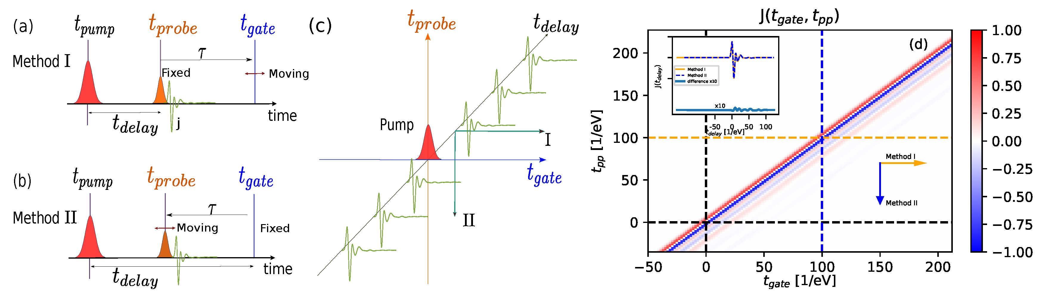
2. Methods

The conductivities, regardless of method, are determined by a functional derivative of the current $J\left(\tau \right)$. The current is obtained by a nonequilibrium Keldysh Green’s function formalism: the self-consistent solution of the Dyson equation on the Keldysh contour [23]. The equations of motion are solved in the superconducting state using a the Nambu Green’s functions [24], with strong electron–phonon interactions mediating the pairing interactions. In addition to electron–phonon interactions (which also scatter in addition to providing the pairing glue), we include impurity scattering to consider the dirty limit of BCS and its resulting signal below the energy of the pairing boson [25,26]. The parameters for the calculation are listed in

Table 1. Parameters used in the simulation.

Phonon frequency $\left(\mathsf{\Omega }\right)$	0.20 eV
Phonon coupling $\left(g^2\right)$	0.12 eV
Impurity coupling (${\langle V_i\rangle }^2$)	0.01 eV
Band parameters	$V_{nn}=0.25$ eV, $\mu =0.0$ eV
Temperature	$\beta =140$ eV${}^{-1}$
Pump pulse	${\omega }_p=1.5$ eV, ${\sigma }_p=8$ eV${}^{-1}$
Probe pulse	$\omega =0.01$ eV, $\sigma =3$ eV${}^{-1}$

. These parameters were chosen for simplicity of calculation and do not represent any specific material; they may be adjusted to simulate real materials. Samples of the resulting currents are shown in Figure 1.

We calculated the conductivity using two methods, as illustrated in Figure 1, and as explained here. In both cases, a current is measured as a function of a time $\tau$, and a functional derivative is performed numerically by Fourier transforming $J\left(\tau \right)$ and the electric field, and taking the ratio. The difference arises in which time is kept fixed, and which is swept to evaluate the current $J\left(\tau \right)$. There are three time points. $t_{pump}$ is the arrival time of the pump pulse, which is used as time zero. $t_{probe}$ is when the probe pulse hits the sample. Finally, $t_{gate}$ is the time when the generated current is measured. The relative time between the pump and the probe is $t_{pp}\equiv t_{pump}-t_{probe}$.

Method I: We compute for fixed values of $t_{pp}$ the ratio $\sigma (\omega ,t_{delay})=\frac{\mathrm{J}(\omega ,t_{pp})}{\mathrm{E}(\omega ,t_{pp})}$, taking the Fourier transform along the $t_{gate}$ axis (in the horizontal direction in Figure 1d). This Method is from a computational perspective straightforward since it simply involves the application of two pulses, and calculating the resulting current.

Method II: $t_{gate}$ is kept at a fixed distance from the pump, and the probe is swept backwards to generate the current $J\left(\tau \right)$. Then, for fixed values of $t_{gate}$ we compute the ratio $\sigma (\omega ,t_{delay})=\frac{\mathrm{J}(\omega ,t_{gate})}{\mathrm{E}(\omega ,t_{gate})}$, taking the Fourier transform along the $\tau$ axis (in the vertical direction in Figure 1d). This Method is computationally more complex since a large number of pump–probe delay sets need to be generated. Here, we have taken data generated from method I and performed Akima spline interpolation [27] to be able to take vertical cuts. The interpolation results are shown in Figure 1d.

The advantage of Method II is that the system dynamics, which are driven by the pump, are always in the same state when the current is measured (at $t_{gate}$). Since the goal of the measurement is to determine the pump-induced dynamics, this method may be able to more selectively observe these and provide better time resolution. In Method I, the effective time resolution for the dynamics is set by the decay time of the current (signal length), which may be long and is generally not known in advance. This long decay time (and thus long effective resolution) produces an averaging over the system dynamics, which may obscure them or in extreme cases hide them if the pump-induced dynamics is comparable to the signal length.

From an experimental viewpoint, there appears to be a preference towards Method I, potentially due to its simplicity and the long relaxation of the excitations compared to the probe width (see, e.g., works by the authors of [1,3,28]. A notable exception is the work by the authors of [22], which discusses the perturbed free induction decay in some detail. As we will demonstrate below, Method II has potential upsides which may prove useful within the experimental context.

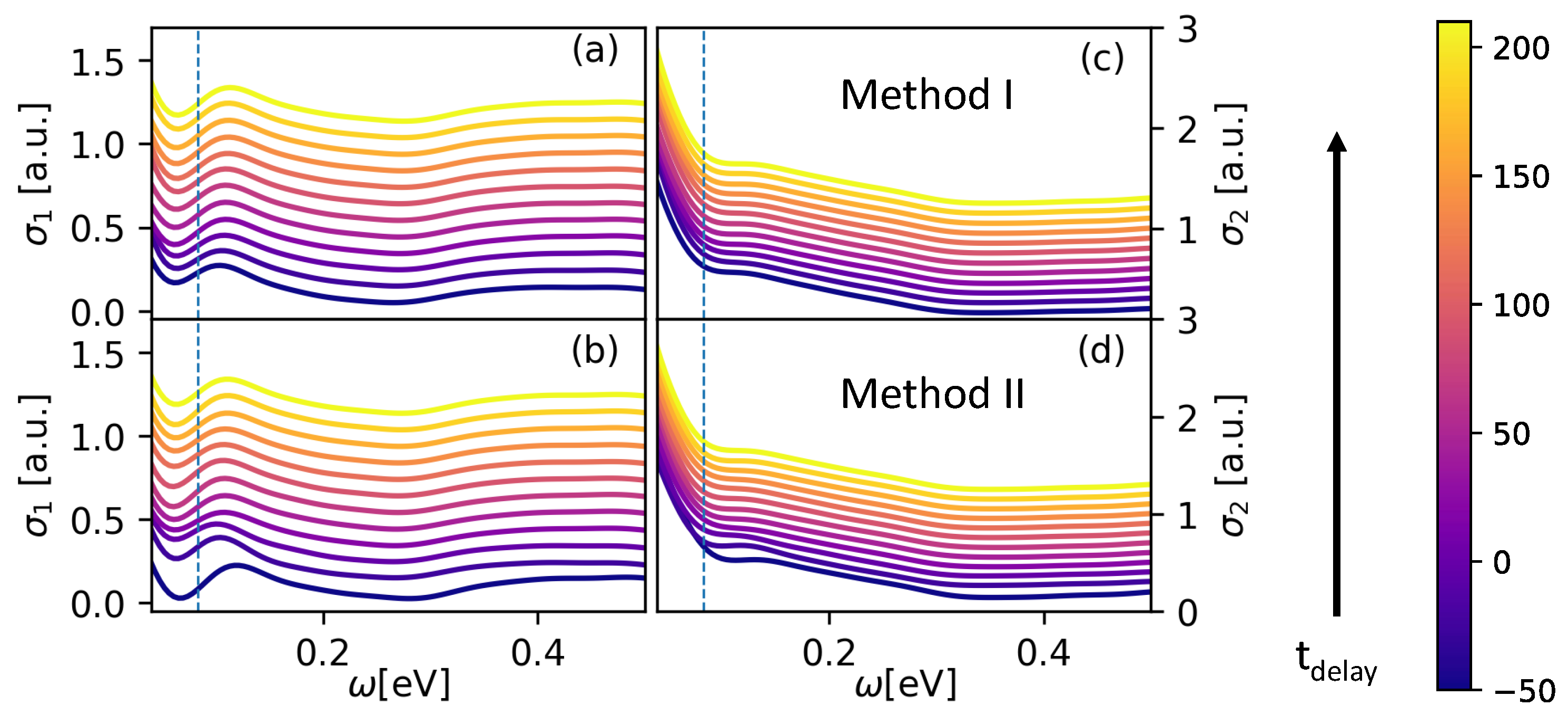
3. Results

To demonstrate the difference between the two approaches, we consider a driven system that has interesting dynamics after the pump—a pumped superconductor. This system shows nontrivial changes in the conductivity, most notably oscillations of the superconducting order. Oscillations are complex when it comes to evaluating them in the optical conductivity since this requires a Fourier transform; in principle, this could simply average over the oscillations and result in a peak in the conductivity rather than any time-dependent behavior, and thus we expect the two methods to show marked differences here.

Figure 2 displays the evolution of the real $\left({\sigma }_1\right)$ and imaginary $\left({\sigma }_2\right)$ parts of the conductivity computed with both Methods as a function of their respective $t_{delay}$ values. The bottom curves corresponding to $t_{delay}=-50.0$ indicate the conductivity components in the equilibrium state, before the pump is applied. The conductivity shows the expected features for a strong-coupling BCS superconductor in the presence of impurity scattering: in ${\sigma }_1$ an upturn at low frequencies in the real part, a step near $2\Delta$, and a minimum at $\mathsf{\Omega }+2\Delta$, and in ${\sigma }_2$ a divergence towards low frequencies. As the pump is applied, the superconductor is partially melted and the features who positions involve $\Delta$ redshift.

In addition to a reduction in the order parameter, the system exhibits Higgs (or Anderson–Higgs) oscillations, which are an oscillatory decay in the relaxation of the excited population of the Cooper pairs in superconducting condensates subject to perturbation by ultrafast pump fields—these were previously discussed based on similar calculations using the nonequilibrium Keldysh formalism [5,19,24,29]. Higgs oscillations arise here due to a time-dependence of the superconducting order parameter and we observe them in the time-dependent conductivity $\sigma (\omega ,t_{delay})$ as time-dependent oscillations of the gap edge and minimum around the phonon energy. It is important to note that a critical aspect of the method for observing the Higgs oscillations with Method I is that the probe current decays. If this were not the case, Method I would effectively have no time resolution, and only oscillations in the peak height would be visible [14].

Following the analysis of Kumar et al. [19], we further investigate the time-evolution of the superconducting order parameter in the aftermath of the pump by considering the dynamics of four time-resolved quantities as functions of $t_{delay}$ for the two methods:

• The probe current minimum, which was demonstrated to be a measure of the order parameter [2,19].
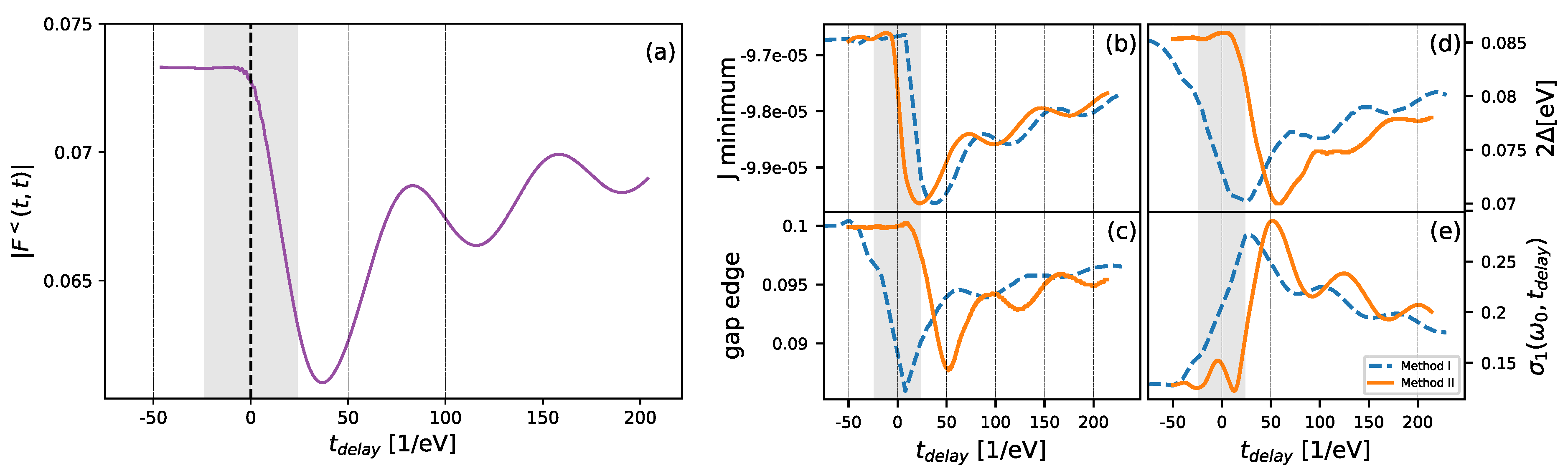
• The location of the gap edge in ${\sigma }_1(\omega ,t_{delay})$, which we define to the the point ${\omega }_{edge}$ on the frequency axis, where the mean of ${\left({\sigma }_1^{sc}/{\sigma }_1^{ns}\right)}_{max}$ and ${\left({\sigma }_1^{sc}/{\sigma }_1^{ns}\right)}_{min}$ is located within the range from $\omega =0$ to $\omega \approx 2{\Delta }_{equilibrium}$.
• The location of the ${\sigma }_1(\omega ,t_{delay})$ minimum about the phonon frequency $\mathsf{\Omega }$ (measured with respect to $\mathsf{\Omega }$).
• The conductivity at a fixed frequency: ${\sigma }_1(\omega =0.083,t_{delay})$.

These four quantities, obtained using both methods, are shown in Figure 3b–e, in the order in which they were discussed. The time axis $t_{delay}$ is provided by $t_{pp}$ and $t_{gate}$ for Methods I and II, respectively. For reference, we also show the anomalous “density”: $F^{<}(t,t)$. This quantity is an instantaneous measure of the superconductivity in the system; in equilibrium it is equivalent to the right hand side of the gap equation, summed over momenta

$$\begin{array}{c}\hfill F^{<}(t,t)=-i\sum _{\mathbf{k}}\frac{{\Delta }_{eq}}{2E_{\mathbf{k}}}tanh\left(\frac{E_{\mathbf{k}}}{2T}\right),\end{array}$$

(5)

where $E_{\mathbf{k}}=\sqrt{{\xi }_{\mathbf{k}}^2+{\Delta }_{eq}^2}$, and T is the temperature. Although this is an imperfect measure of the amount of superconductivity in the system because it only captures the amplitude of the order and not the phase [30], it has shown to be correlated with the spectral gap and its dynamics [24].

There are several differences between the two methods, which we will now discuss. In all cases, the curves show a suppression of the gap, followed by the characteristic Higgs oscillations, which were discussed in detail in the work by the authors of [19].

However, the most striking difference is an apparent horizontal shift between the curves. For the Fourier transformed quantities obtained from the conductivity panels (c–e)), the dynamics using Method I occur earlier by approximately 50 eV${}^{-1}$. These shifts are due to a mechanism termed “perturbed free induction decay,” where for negative times the pump arrives while the probe-induced current is still decaying, causing an earlier than expected observation of changes in the conductivity due to the pump (see, e.g., the third current in Figure 1c). This is in particular relevant for low-frequency features in the conductivity, which by nature require long time signals. This effect produces both the earlier appearance of the maximal change and following shift of the Higgs oscillations, but also the appearance of changes before the pump is active. In contrast, Method II does not have this artifact—the maximal change occurs more closely to where $F^{<}(t,t)$ reaches its maximal change.

In the case of the minimum current, the reverse occurs: the current from Method II reaches its largest change earlier than Method I. Here, this is due to the delay in when the minimum current occurs: it appears some fixed time after the pump, which in Method I shifts the time to higher values. In comparing the currents, Method II more correctly identifies when the change in the gap occurs—it stops decreasing when the pump is off.

4. Summary

We have evaluated the conductivity of a pumped superconductor with two experimentally accessible methods. The methods involve two arrangements of the three times involved in an optical pump–probe experiment: the pump, probe, and gate times. The conductivities obtained from the two methods are qualitatively similar, but differ in some key details. The pumped superconductor typically exhibits a suppression, followed by recovery with Higgs oscillations. Both methods discussed here exhibit these features, but with notable differences. First, the (simpler) Method I observes “perturbed free induction” changes before the pump arrives. More generally, due to an effective averaging over the current decay time, Method I’s features are somewhat smeared. In contrast, Method II has sharp changes, and exhibits no changes before the pump arrives. Our results suggest that Method II offers improved time resolution over Method I, although Method I does reproduce some of the observed effects.

5. Materials and Methods

The simulations were performed with the self-consistent nonequilibrium Keldysh formalism described in the work by the authors of [23]. The Holstein Hamiltonian is used to simulate a phonon-mediated, s-wave superconductor on 2D square lattice

$$\begin{array}{cc}\hfill \mathcal{H}& =\sum _{\mathbf{k},\sigma }\xi \left(\mathbf{k}\right)c_{\mathbf{k},\sigma }^{†}{c}_{\mathbf{k},\sigma }^{\phantom{†}}+\mathsf{\Omega }\sum _{\mathbf{q}}\left(b_{\mathbf{q}}^{†}{b}_{\mathbf{q}}^{\phantom{†}}+\frac{1}{2}\right)+\frac{g}{\sqrt{N}}\sum _{\begin{array}{c}\sigma \\ \mathbf{k},\mathbf{q}\end{array}}{c}_{\mathbf{k}+\mathbf{q},\sigma }^{†}{c}_{\mathbf{k},\sigma }^{\phantom{†}}\left(b_{\mathbf{q}}^{\phantom{†}}+b_{-\mathbf{q}}^{†}\right)+\sum _{i,\sigma }{V}_i{c}_{i,\sigma }^{†}{c}_{i,\sigma }\hfill \end{array}$$

(6)

Here, $\xi \left(\mathbf{k}\right)$ ($=-2{\mathrm{V}}_{\mathrm{nn}}\left[cos\left(k_x\right)+cos\left(k_y\right)\right]-\mu$) is the nearest neighbor tight-binding energy dispersion with hopping parameter $V_{nn}$ measured relative to the chemical potential $\mu$, $c_{\mathbf{k}}^{†},c_{\mathbf{k}}^{\phantom{†}}$ ($b_{\mathbf{q}}^{†},b_{\mathbf{q}}$) are the standard creation and annihilation operators for an electron (phonon), g is the momentum-independent e-ph coupling constant, and $\mathsf{\Omega }$ is the frequency for the Einstein phonon. $V_i$ is the coupling between electrons and impurities which are distributed randomly on lattice sites.

We used the parameters listed in Table 1. An oscillating Gaussian pump pulse with a width ${\sigma }_p$ and a central frequency ${\omega }_p$ was applied, followed by a probe pulse of similar shape but with $\sigma$ and $\omega$ as width and central frequency, respectively. As illustrated in Figure 1, the pump–probe delay time was varied. The generated data was interpolated with Akima splines [27] before taking Fourier transforms in the two directions indicated in the figure.

The software and data used in this manuscript is publicly available in the work by the authors of [31].

References

- Mitrano, M.; Cantaluppi, A.; Nicoletti, D.; Kaiser, S.; Perucchi, A.; Lupi, S.; Di Pietro, P.; Pontiroli, D.; Riccò, M.; Clark, S.R.; et al. Possible light-induced superconductivity in K3C60 at high temperature. Nature 2016, 530, 461–464. [Google Scholar] [CrossRef] [PubMed]
- Matsunaga, R.; Hamada, Y.I.; Makise, K.; Uzawa, Y.; Terai, H.; Wang, Z.; Shimano, R. Higgs Amplitude Mode in the BCS Superconductors Nb1−xTixN Induced by Terahertz Pulse Excitation. Phys. Rev. Lett. 2013, 111, 057002. [Google Scholar] [CrossRef] [PubMed]
- Matsunaga, R.; Tsuji, N.; Fujita, H.; Sugioka, A.; Makise, K.; Uzawa, Y.; Terai, H.; Wang, Z.; Aoki, H.; Shimano, R. Light-induced collective pseudospin precession resonating with Higgs mode in a superconductor. Science 2014, 345, 1145–1149. [Google Scholar] [CrossRef] [PubMed]
- Murakami, Y.; Werner, P.; Tsuji, N.; Aoki, H. Multiple amplitude modes in strongly coupled phonon-mediated superconductors. Phys. Rev. B 2016, 93, 094509. [Google Scholar] [CrossRef]
- Tsuji, N.; Murakami, Y.; Aoki, H. Nonlinear light–Higgs coupling in superconductors beyond BCS: Effects of the retarded phonon-mediated interaction. Phys. Rev. B 2016, 94, 224519. [Google Scholar] [CrossRef]
- Kennes, D.M.; Wilner, E.Y.; Reichman, D.R.; Millis, A.J. Nonequilibrium optical conductivity: General theory and application to transient phases. Phys. Rev. B 2017, 96, 054506. [Google Scholar] [CrossRef]
- Silaev, M. Nonlinear electromagnetic response and Higgs-mode excitation in BCS superconductors with impurities. Phys. Rev. B 2019, 99, 224511. [Google Scholar] [CrossRef]
- Murotani, Y.; Shimano, R. Nonlinear optical response of collective modes in multiband superconductors assisted by nonmagnetic impurities. Phys. Rev. B 2019, 99, 224510. [Google Scholar] [CrossRef]
- Shimano, R.; Tsuji, N. Higgs Mode in Superconductors. arXiv 2019, arXiv:1906.09401. [Google Scholar]
- Jujo, T. Quasiclassical Theory on Third-Harmonic Generation in Conventional Superconductors with Paramagnetic Impurities. J. Phys. Soc. Jpn. 2017, 87, 024704. [Google Scholar] [CrossRef]
- Cea, T.; Castellani, C.; Seibold, G.; Benfatto, L. Nonrelativistic Dynamics of the Amplitude (Higgs) Mode in Superconductors. Phys. Rev. Lett. 2015, 115, 157002. [Google Scholar] [CrossRef]
- Cea, T.; Castellani, C.; Benfatto, L. Nonlinear optical effects and third-harmonic generation in superconductors: Cooper pairs versus Higgs mode contribution. Phys. Rev. B 2016, 93, 180507. [Google Scholar] [CrossRef]
- Udina, M.; Cea, T.; Benfatto, L. Theory of coherent oscillations detection in THz pump-probe spectroscopy: From phonons to electronic collective modes. arXiv 2019, arXiv:1907.06092. [Google Scholar]
- Krull, H.; Manske, D.; Uhrig, G.S.; Schnyder, A.P. Signatures of nonadiabatic BCS state dynamics in pump-probe conductivity. Phys. Rev. B 2014, 90, 014515. [Google Scholar] [CrossRef]
- Orenstein, J.; Dodge, J.S. Terahertz time-domain spectroscopy of transient metallic and superconducting states. Phys. Rev. B 2015, 92, 134507. [Google Scholar] [CrossRef]
- Shao, C.; Tohyama, T.; Luo, H.G.; Lu, H. Numerical method to compute optical conductivity based on pump-probe simulations. Phys. Rev. B 2016, 93, 195144. [Google Scholar] [CrossRef]
- Eckstein, M.; Kollar, M. Theory of time-resolved optical spectroscopy on correlated electron systems. Phys. Rev. B 2008, 78, 205119. [Google Scholar] [CrossRef]
- Tsuji, N.; Oka, T.; Aoki, H. Nonequilibrium Steady State of Photoexcited Correlated Electrons in the Presence of Dissipation. Phys. Rev. Lett. 2009, 103, 047403. [Google Scholar] [CrossRef] [PubMed]
- Kumar, A.; Kemper, A. Higgs Oscillations in time-resolved Optical Conductivity. arXiv 2019, arXiv:1902.09549. [Google Scholar]
- Kindt, J.T.; Schmuttenmaer, C.A. Theory for determination of the low-frequency time-dependent response function in liquids using time-resolved terahertz pulse spectroscopy. J. Chem. Phys. 1999, 110, 8589–8596. [Google Scholar] [CrossRef]
- Němec, H.; Kadlec, F.; Kužel, P. Methodology of an optical pump-terahertz probe experiment: An analytical frequency-domain approach. J. Chem. Phys. 2002, 117, 8454–8466. [Google Scholar] [CrossRef]
- Coslovich, G.; Kemper, A.F.; Behl, S.; Huber, B.; Bechtel, H.A.; Sasagawa, T.; Martin, M.C.; Lanzara, A.; Kaindl, R.A. Ultrafast dynamics of vibrational symmetry breaking in a charge-ordered nickelate. Sci. Adv. 2017, 3, e1600735. [Google Scholar] [CrossRef] [PubMed]
- Kemper, A.; Sentef, M.; Moritz, B.; Freericks, J.; Devereaux, T. Effect of dynamical spectral weight redistribution on effective interactions in time-resolved spectroscopy. Phys. Rev. B 2014, 90, 075126. [Google Scholar] [CrossRef]
- Kemper, A.F.; Sentef, M.A.; Moritz, B.; Freericks, J.K.; Devereaux, T.P. Direct observation of Higgs mode oscillations in the pump-probe photoemission spectra of electron-phonon mediated superconductors. Phys. Rev. B 2015, 92, 224517. [Google Scholar] [CrossRef]
- Mattis, D.C.; Bardeen, J. Theory of the Anomalous Skin Effect in Normal and Superconducting Metals. Phys. Rev. 1958, 111, 412–417. [Google Scholar] [CrossRef]
- Zimmermann, W.; Brandt, E.H.; Bauer, M.; Seider, E.; Genzel, L. Optical conductivity of BCS superconductors with arbitrary purity. Phys. C Supercond. 1991, 183, 99–104. [Google Scholar] [CrossRef]
- Akima, H. A new method of interpolation and smooth curve fitting based on local procedures. J. ACM 1970, 17, 589–602. [Google Scholar] [CrossRef]
- Yang, X.; Vaswani, C.; Sundahl, C.; Mootz, M.; Gagel, P.; Luo, L.; Kang, J.H.; Orth, P.P.; Perakis, I.E.; Eom, C.B.; et al. Terahertz-light quantum tuning of a metastable emergent phase hidden by superconductivity. Nat. Mater. 2018, 17, 586–591. [Google Scholar] [CrossRef] [PubMed]
- Kemper, A.; Sentef, M.A.; Moritz, B.; Devereaux, T.; Freericks, J. Review of the Theoretical Description of Time-Resolved Angle-Resolved Photoemission Spectroscopy in electron-phonon Mediated Superconductors. Annalen der Physik 2017, 529, 1600235. [Google Scholar] [CrossRef]
- Stahl, C.; Eckstein, M. Noise correlations in time- and angle-resolved photoemission spectroscopy. Phys. Rev. B 2019, 99, 241111. [Google Scholar] [CrossRef]
- GRENDEL Development Team. Available online: https://github.com/kemperlab/grendel/ (accessed on 26 August 2019).