Article

Implementation of an Enhanced Crayfish Optimization Algorithm

1
College of Electrical and Computer Science, Jilin Jianzhu University, Changchun 130000, China
2
Jilin Provincial Department of Human Resources and Social Security, Changchun 130000, China
*
Author to whom correspondence should be addressed.
Biomimetics 2024, 9(6), 341; https://doi.org/10.3390/biomimetics9060341
Submission received: 12 April 2024 / Revised: 21 May 2024 / Accepted: 22 May 2024 / Published: 4 June 2024
(This article belongs to the Special Issue Bioinspired Algorithms)

Abstract

:
This paper presents an enhanced crayfish optimization algorithm (ECOA). The ECOA includes four improvement strategies. Firstly, the Halton sequence was used to improve the population initialization of the crayfish optimization algorithm. Furthermore, the quasi opposition-based learning strategy is introduced to generate the opposite solution of the population, increasing the algorithm’s searching ability. Thirdly, the elite factor guides the predation stage to avoid blindness in this stage. Finally, the fish aggregation device effect is introduced to increase the ability of the algorithm to jump out of the local optimal. This paper performed tests on the widely used IEEE CEC2019 test function set to verify the validity of the proposed ECOA method. The experimental results show that the proposed ECOA has a faster convergence speed, greater performance stability, and a stronger ability to jump out of local optimal compared with other popular algorithms. Finally, the ECOA was applied to two real-world engineering optimization problems, verifying its ability to solve practical optimization problems and its superiority compared to other algorithms.

1. Introduction

Engineering problems have become increasingly complex [1] with the rapid development of engineering technology. As a result, more and more issues need to be optimized, making the importance of optimization increasingly prominent [2]. Traditional optimization algorithms, such as linear programming [3], gradient descent [4], and the simplex method [5], are often used to solve these problems in the past. Although they performed well in solving simple problems, their limitations became more apparent as engineering challenges and data processing requirements increased. Traditional algorithms are difficult to solve high-dimensional, nonlinear, or discrete optimization problems. Therefore, the swarm intelligent optimization algorithm [6] was developed, simulating the behavior of biological groups in nature to seek the optimal solution through cooperation and information exchange between individuals [7]. The swarm intelligence algorithms have more vital global optimization ability, robustness, and adaptability and can deal with various complex optimization tasks compared to traditional algorithms. These problems are all complex, and a swarm intelligent optimization algorithm can help find the optimal or approximate optimal solution [8], improving the solving efficiency and solution quality.
Many swarming optimization algorithms have been proposed recently due to their simplicity and strong optimization capabilities [9]. These algorithms include ant colony algorithm [10] (ACO) inspired by the foraging behavior of ants in nature, particle swarm optimization algorithm [11] (PSO) that simulates bird foraging behavior, and whale optimization algorithm [12] (WOA) that simulates the unique search methods and trapping mechanisms of humpback whales, among others. Although these standard swarming algorithms have been successful in many problems, they may still face some challenges in some cases [13]. Scholars have proposed several improved versions to address these challenges and improve the performance of swarm intelligence algorithms. For instance, Hadi Moazen et al. [14] identified the shortcomings of the PSO and developed an improved PSO-ELPM algorithm with elite learning, enhanced parameter updating, and exponential mutation operators. This algorithm balances the exploration and development capabilities of the PSO and produces higher accuracy at an acceptable time complexity, as demonstrated by the CEC 2017 test set. Similarly, Ya Shen et al. [15] proposed the MEWOA algorithm, which divides individual whales into three subpopulations and adopts different renewal methods and evolutionary strategies. This algorithm has been applied to global optimization and engineering design problems, and its effectiveness and competitiveness have been verified. Furthermore, Fang Zhu et al. [16] found that the Dung Beetle optimization algorithm (DBO) was prone to falling into local optima in the late optimization period. They proposed the Dung Beetle search algorithm (QHDBO) based on quantum computing and a multi-strategy mixture to address this issue. The strategy’s effectiveness was verified through experiments, which significantly improved the convergence speed and optimization accuracy of the DBO. These proposed and improved optimization algorithms significantly promote the development of swarm intelligence algorithms and make their performance better, allowing them to be applied to optimization problems in various fields, such as workshop optimization scheduling [17], microgrid optimization scheduling [18], vehicle path planning [19], engineering design [20], and wireless sensor layout [21].
The crayfish optimization algorithm [22] (COA) was proposed in September 2023 as a new swarm intelligence optimization algorithm inspired by the summer, competition, and predatory behavior of crayfish. There is intense competition in global optimization and engineering optimization. However, experiments have found that the convergence rate could be slower in some problems and has fallen into local optimal problems. This paper presents four strategies to improve it and comprehensively improve the optimization performance of the COA. The main contributions of this paper are as follows:
(1)
An enhanced crayfish optimization algorithm (ECOA) is proposed by mixing four improvement strategies. Halton sequence was introduced to improve the population initialization process of COA, which made the initial population distribution of crayfish more uniform and increased the initial population’s diversity and the early COA’s convergence rate. Before crayfish began to summer resort, compete, and predate, QOBL was applied to the COA population, which was conducive to increasing the search range of the population and improving the quality of candidate solutions to accelerate the convergence rate. There is a certain blindness in this process, and elite factors are introduced to guide the crayfish because crayfish can directly ingest food when the size of the food is appropriate. This paper introduces the fish device aggregation effect (FADs) in the marine predator algorithm (MPA) into the predation phase of crayfish to enhance the ability of COA to jump out of local optimality.
(2)
The proposed ECOA solves the widely used IEEE CEC2019 test function set and compares it with four standard swarm intelligence algorithms, four improved swarm intelligence algorithms, and crayfish optimization algorithms, respectively. Five experiments were carried out: numerical experiment, iterative curve analysis, box plot analysis, the Wilcoxon rank sum test, and ablation experiments. The experimental results show that the proposed ECOA is competitive and compared to similar algorithms, it has faster convergence speed, higher convergence accuracy, and stronger ability to jump out of local optima.
(3)
Using the ECOA for practical optimization problems in the three-bar truss design and pressure vessels design, and comparing it with other algorithms. The ECOA shows higher convergence accuracy, faster convergence speed, and higher stability compared to other algorithms.
The rest of this paper is arranged as follows: Part 2 introduces the standard crayfish optimization algorithm (COA), Part 3 details the proposed enhanced crayfish optimization algorithm (ECOA), Part 4 tests the effectiveness of the ECOA and its superiority over other optimization algorithms through five experiments, Part 5 applies the ECOA to practical engineering optimization problems and Part 6 is the conclusion and future work.

2. The Crayfish Optimization Algorithm (COA)

The crayfish optimization algorithm (COA) is a novel swarm intelligence optimization algorithm inspired by crayfish’s summer heat, competition, and predation behavior. Crayfish are arthropods of the shrimp family that live in various freshwater areas. Research has shown that crayfish behave differently in different ambient temperatures. In the mathematical modeling of COA, the heat escape, competition, and predation behavior are defined as three distinct stages, and the optimization algorithm is controlled to enter different stages by defining different temperature intervals. Among them, the summer stage is the exploration stage of COA, the competition stage, and the foraging stage is the development stage of COA. The steps of the COA are described in detail below.

2.1. Population Initialization

The COA is a population-based algorithm that starts with population initialization to provide a suitable starting point for the subsequent optimization process. In the modeling of COA, the location of each crayfish represents a candidate solution to a problem, which has D dimension, and the population location of N crayfish constitutes a group of candidate solutions X, whose expression is shown as Equation (1).
X = X 1 X i X N = X 1,1 X 1 , j X 1 , D X i , 1 X N , 1 X i , j X N , j X i , D X N , D N × D
where X is the location of the initial crayfish population, N is the number of crayfish population, D is the dimension of the problem, and X i , j is the initial location of the i crayfish in the j dimension, which is generated in the search space of the problem randomly, and the specific expression of X i , j is shown in Equation (2).
X i , j = l b j + u b j l b j · r , i = 1,2 , , N ; j = 1,2 , , D
where l b j is the lower bound of the j-dimension of the problem variable in the search space, u b j is the upper bound, and r is the uniformly distributed random number belonging to [0, 1].

2.2. Define Temperature and Crawfish Food Intake

At different ambient temperatures, crayfish will enter different stages. The crayfish will enter the summer stage when the temperature is above 30 °C. Crayfish have assertive predation behavior between 15 °C and 30 °C, with 25 °C being the optimal temperature. Their food intake is also affected by temperature and is approximately normal as temperature changes. In COA, the temperature T e m p is defined as Equation (3).
T e m p = 20 + r · 15
where T e m p is the ambient temperature. The mathematical expression of food intake P of crayfish is shown in Equation (4).
P = C 1 · 1 2 π · σ · exp T e m p μ 2 2 σ 2
where μ is the optimal temperature and C 1 and σ are used to control the food intake of crayfish at different ambient temperatures.

2.3. Summer Phase

When the temperature T e m p is higher than 30 °C, crayfish will choose X s h a d e cave for heat escape, which is the heat escape stage of the COA. The mathematical definition of X s h a d e cave is shown in Equation (5).
X s h a d e = 0.5 · X G + X L
where X G is the optimal position obtained by the algorithm iteration so far, and X L is the optimal position of the current crayfish population.
There may be competition for crawfish to get into the heat. Multiple crayfish will compete for the same burrow to escape the heat if there are many crayfish and few burrows. This will not be the case if there are more caves. A random number between 0 and 1, r a n d is used to determine whether a race has occurred in the COA. When the random number r a n d < 0.5 , no other crayfish compete for the cave, and crayfish can directly enter the cave to escape the heat. The mathematical expression of this process is shown in Equation (6).
X i , j t + 1 = X i , j t + C 2 · r · X s h a d e X i , j t
where t is the current number of iterations, X i , j t is the current position of the i crayfish in the j th dimension, t + 1 represents the number of iterations of the next generation, r is a random number [0, 1], and the value of C 2 decreases with the increase in iterations, as expressed in Equation (7).
C 2 = 2 t T , t = 1,2 , , T
where T is the maximum number of iterations of the algorithm.

2.4. Competition Phase

Multiple crayfish will compete for a cave and enter the competition stage when the temperature T e m p is higher than 30 °C and the random number r a n d 0.5 . At this stage, the position of the crayfish is updated, as shown in Equation (8).
X i , j t + 1 = X i , j t X z , j t + X s h a d e
where z is a random crayfish in the population, and its expression is shown in Equation (9).
z = r o u n d r · ( N 1 ) + 1
where r is the random number belonging to [0, 1], and r o u n d · is the integer function.

2.5. Predation Stage

The crayfish will hunt and eat food when the temperature T e m p 30   ° C . The Crawfish move towards their food and eat it. The food location X f o o d is defined in Equation (10).
X f o o d = X G
The crayfish will judge the size of the food to adopt different ways before ingesting food. The size Q of food is defined in Equation (11). The crayfish will tear the food with their claws first if the food is too large, and alternate eating with their second and third walking feet.
Q = C 3 · r · F i t n e s s i F i t n e s s f o o d
where C 3 is the food factor, representing the maximum value of food, and the value is constant 3; F i t n e s s i is the fitness value of the i crayfish, that is the objective function value; F i t n e s s f o o d represents the fitness value of the food location X f o o d . The Crayfish judge the size of their food by the size C 3 of their maximum food. When the size of the food Q > C 3 + 1 / 2 , the food is too large, and the tiny dragon will use chelates (shrimp claws, the first pair of feet) to tear the food; the mathematical expression is as Equation (12).
X f o o d = exp 1 Q · X f o o d
After that, the crayfish will alternate feeding with the second and third feet, a process simulated in the COA using sine and cosine functions, as shown in Equation (13).
X i , j t + 1 = X i , j t + X f o o d · P · cos 2 · π · r sin 2 · π · r
where P is the food intake and r is the random number belonging to [0, 1].
The food size is appropriate and crayfish can be directly ingested when Q C 3 + 1 / 2 , and the position update expression is shown in Equation (14).
X i , j t + 1 = P · X i , j t X f o o d + P · r · X i , j t
where r is a random number belonging to [0, 1].

3. The Enhanced Crayfish Optimization Algorithm (ECOA)

This section describes the proposed enhanced crayfish optimization algorithm (ECOA). Because the crawfish optimization algorithm (COA) has defects in slow convergence speed and easy falling into local areas, this paper adopts four strategies to improve it and comprehensively enhance the optimization performance of the crawfish optimization algorithm. Firstly, the Halton sequence is used to improve the population initialization so that the initial population is more evenly distributed in the search space. Secondly, quasi opposition-based learning strategy is introduced to generate the quasi-oppositional solution of the population, and the next-generation population is selected by greedy strategy, which increases the search space and enhances the diversity of the crayfish population. Thirdly, the foraging stage is improved, and the elite guiding factor is introduced to enhance the optimization rate of this stage. Finally, after the foraging stage, the vortex effect of the marine predator algorithm is introduced to strengthen the ability of the algorithm to jump out of the local optimal. Specific enhancement strategies are as follows.

3.1. Halton Sequence Population Initialization

Generally, population initialization in swarm intelligent optimization algorithms creates initial solutions that can converge to better solutions through continuous iteration [23]. This process forms the basis of algorithm iteration, and the population initialization quality directly affects the algorithm’s iteration speed and global optimization ability. In a standard COA, crayfish populations are generated randomly. Although this initialization method is simple and easy to implement, it may lead to uneven distribution of small and medium-sized lobsters in the population, and the population cannot cover the entire search space well, resulting in slow convergence of the algorithm and even falling into local optimal prematurely.
In contrast, the Halton sequence [24] makes the generated points evenly distributed throughout the search space as a low difference [25] numerical sequence. It differs from random sequences that create different points each time because of its deterministic nature. This paper uses the Halton sequence to replace the original random initialization strategy. This alternative can make the initial population cover the whole search space more evenly, improve the diversity of the population, and speed up the algorithm’s convergence. The expression for the initial location of each crayfish produced by population initialization based on the Halton sequence is shown in Equation (15).
X i , j = l b j + u b j l b j · H a l t o n s e t , i = 1,2 , , N ; j = 1,2 , , D
where H a l t o n s e t is a value based on the Halton sequence.

3.2. Quasi Opposition-Based Learning

Opposition-based learning [26] (OBL) was first proposed by Tizhoosh in 2005 and has been widely used to improve swarm intelligence optimization algorithms in subsequent studies. The concept is to generate the opposite solution of the current population, and by comparing the current solution and the opposite solution, retain the better candidate solution of the two as the next-generation population. OBL proposed that the opposition values of the current candidate solutions may be closer to the optimal solution, and the process is conducive to increasing the search range of the population and improving the quality of the candidate solutions. The position expression of the generated opposition solutions is shown in Equation (16).
X i O B L = l b + u b X i
where lb is the lower bound of the problem variable in the search space, and u b is the upper bound.
There are also limitations. Inverse learning can improve the algorithm’s convergence speed in the early iteration stage, although some improvements show good performance. The inverse solution generated in the late iteration stage may slow down the algorithm speed due to the excessive position change. Quasi opposition-based learning [27] (QOBL) is a more effective oppositional learning strategy evolved from OBL. It requires that the opposite solution be close to the center M of the search space, not the opposite value; the value of M is shown in Equation (17). Figure 1 shows the position schematic of the generated quasi-opposition and the ordinary opposition solutions. It can be seen from the figure that the position of the quasi-opposition solution generated by QOBL is between the opposition solution and the center of the search space.
The expression X i Q O B L for the position of the quasi-opposite solution generated by QOBL is shown in Equation (18).
M = l b + u b / 2
X i Q O B L = M + X i O B L M · r , X i < M X i O B L + M X i O B L · r , e l s e
where r is the uniformly distributed random number belonging to [0, 1].

3.3. Elite Steering Factor

Formula (14) describes that crayfish can directly ingest food when the size of the food is appropriate, and there is a certain blindness in this process of crayfish. Therefore, this paper introduces the elite factor [28] to guide the position update, as shown in Equation (19). With its replacement Formula (14), the algorithm can be guided to converge faster and improve the optimization accuracy to a certain extent. The boundary value is taken if the crayfish position updated by Equation (19) is outside the search boundary.
X i , j t + 1 = P · X i , j t X f o o d + P · r · X L
where X L is the optimal position of the current crayfish population, that is the elite.

3.4. Vortex Formation and Fish Aggregation Device Effect

Modeling the effects of fish aggregating devices ( F A D s ) [29] was first proposed in the marine predator algorithm. In modeling the F A D s effect, the individual position of the population may produce a long jump, which can help the algorithm jump out of the local optimal solution. In this paper, the F A D s effect is added to the predation phase of COA. Suppose the crawfish fitness f i t n e s s i t + 1 after the update of Equation (19) is not as good as the fitness f i t n e s s i t of the previous generation, the positions of these crawfish are disturbed according to the F A D effect, and the mathematical expression of this process is shown in (20).
X i t + 1 = X i t + C F · l b + r · u b l b · U ,   r F A D s X i t + F A D s · 1 r · X r 1 t X r 2 t ,   r > F A D s
where X i t is the current position of the i crayfish, X i t + 1 represents the position of the next generation, the value of F A D s is 0.2, U is a binary vector whose value is between 0 and 1, r is a uniformly distributed random number belonging to [0, 1], and X r 1 t and X r 2 t are the positions of two random individuals in the current population.

3.5. Pseudo-Code of the ECOA

The pseudo-code of the ECOA proposed in this paper is shown in Algorithm 1.
Algorithm 1. The pseudo-code of the ECOA
Initialize population size N , number of iterations T , problem dimension D
for  i = 1: N
  for  j = 1: D
     Generate the initial population individual position according to Equation (15)
  end
end
Calculate the fitness value of the population to obtain the values of X G and X L
While  t < T
  Define the ambient temperature T e m p through Equation (3)
  for  i = 1: N
       Crayfish perform QOBL according to Equation (18)
  end
  Choosing to retain crayfish populations with better fitness for the next generation
  if  T e m p > 30
    Define the cave location X s h a d e according to Equation (5)
    if  r a n d > 0.5
       Crayfish undergo the summer retreat stage according to Equation (6)
    else
       Crayfish compete in stages according to Equation (8)
    end
  else
    Define food intake P and size Q through Equations (4) and (11), respectively
    if  Q > 2
       Crayfish shred food according to Equation (12)
       Crayfish ingest food according to Equation (13)
    else
       Crayfish can directly consume food according to Equation (19)
       if f i t n e s s i t + 1 < f i t n e s s i t
       The position of crayfish remains unchanged
       else
       Update the F A D s effect of crayfish based on Equation (20)
       end
    end
  end
Perform boundary processing
Update fitness values, X G and X L values
    t = t + 1
end

3.6. Analysis of Computational Time Complexity of the ECOA

In the standard crayfish optimization algorithm (COA), N is the number of crayfish populations, D is the number of problem variables, and T is the maximum number of iterations in the algorithm. The time complexity of the standard crayfish optimization algorithm is O ( N × D × T ) . In the ECOA, the complexity of the introduced Halton sequence initialization is O ( N × D ) , which is the same as the original random initialization. The complexity of quasi opposition-based learning is also O ( N × D ) . The elite factor introduced during the predation phase is an improvement on the established steps of the original algorithm and will not increase the complexity of the original algorithm. Due to the fact that only a small number of crayfish undergo the F A D s effect, its time complexity is much smaller than O ( N × D ) . In summary, the overall complexity of the ECOA is less than O ( N × D × ( 3 + T ) ) . Therefore, the proposed ECOA does not increase much computational complexity and is on the same order of magnitude as the complexity of COA.

4. The ECOA Effectiveness Test Experiment

4.1. Experimental Scheme

In this section, we conduct simulation experiments on the IEEE CEC2019 [30] test function set to verify the proposed enhanced crayfish optimization algorithm’s (ECOA) optimization performance. The name, dimension D, range and optimal value information of the IEEE CEC2019 test function set are shown in Table 1, which contains 10 minimally optimized single-objective test functions, which is highly challenging.
This paper compares the ECOA with a nine-population intelligent optimization algorithm. They include advanced standard optimization algorithms: the particle swarm optimization algorithm (PSO), the Aquila Optimizer [31] (AO), the Beluga Optimization algorithm [32] (BWO), the golden jackal optimization algorithm [33] (GJO), and the crayfish optimization algorithm (COA). Recently, advanced optimization algorithms have been proposed: the sine-cosine chaotic Harris Eagle Optimization Algorithm [34] (CSCAHHO), the Adaptive slime fungus algorithm [35] (AOSMA), the mixed arithmetic-trigonometric optimization algorithm [36] (ATOA), and the Adaptive Gray Wolf Optimizer [37] (AGWO). These algorithms include the most widely used algorithms, recently proposed algorithms, and four highly advanced improved algorithms. They have demonstrated strong optimization performance in previous research, and compared with these algorithms, they better reflect the excellent optimization ability of the proposed ECOA. The population of all algorithms is set to 30, the maximum number of iterations is set to 2000, and the critical parameters of each algorithm are set using the original algorithm parameters, as shown in Table 2.
All experiments were conducted on a computer with a Windows 10 operating system, a Intel(R) Core (TM) i7-7700HQ 2.80 GHz CPU and 16 GB memory. The simulation experiment platform used is Matlab R2022a. This experiment is divided into five parts: numerical experiment analysis, iterative curve analysis, box plot analysis, the Wilcoxon rank sum tests and ablation experiments. The above experimental system verifies the effectiveness and superiority of the ECOA.

4.2. Numerical Experiment and Analysis

In this section, the results of each algorithm running 30 times on CEC2019 are counted, and the statistical indicators include the best value (Best), the mean value (Mean), and the standard deviation (Std). The numerical experimental results of the ECOA and other comparisons are shown in Table 3. In addition to the PSO and the GJO, the ECOA and other algorithms have an optimal value of 1 on F1. The average and optimal values obtained by the ECOA are the minimum, and the minimum standard deviation is obtained on most test functions on F2–F9. By comparing the best value with the average value, it can be seen that the proposed ECOA algorithm has higher optimization accuracy than other algorithms. From the statistical results of the standard deviation, it can be seen that the ECOA proposed in most test functions has higher robustness.

4.3. Iterative Curve Analysis

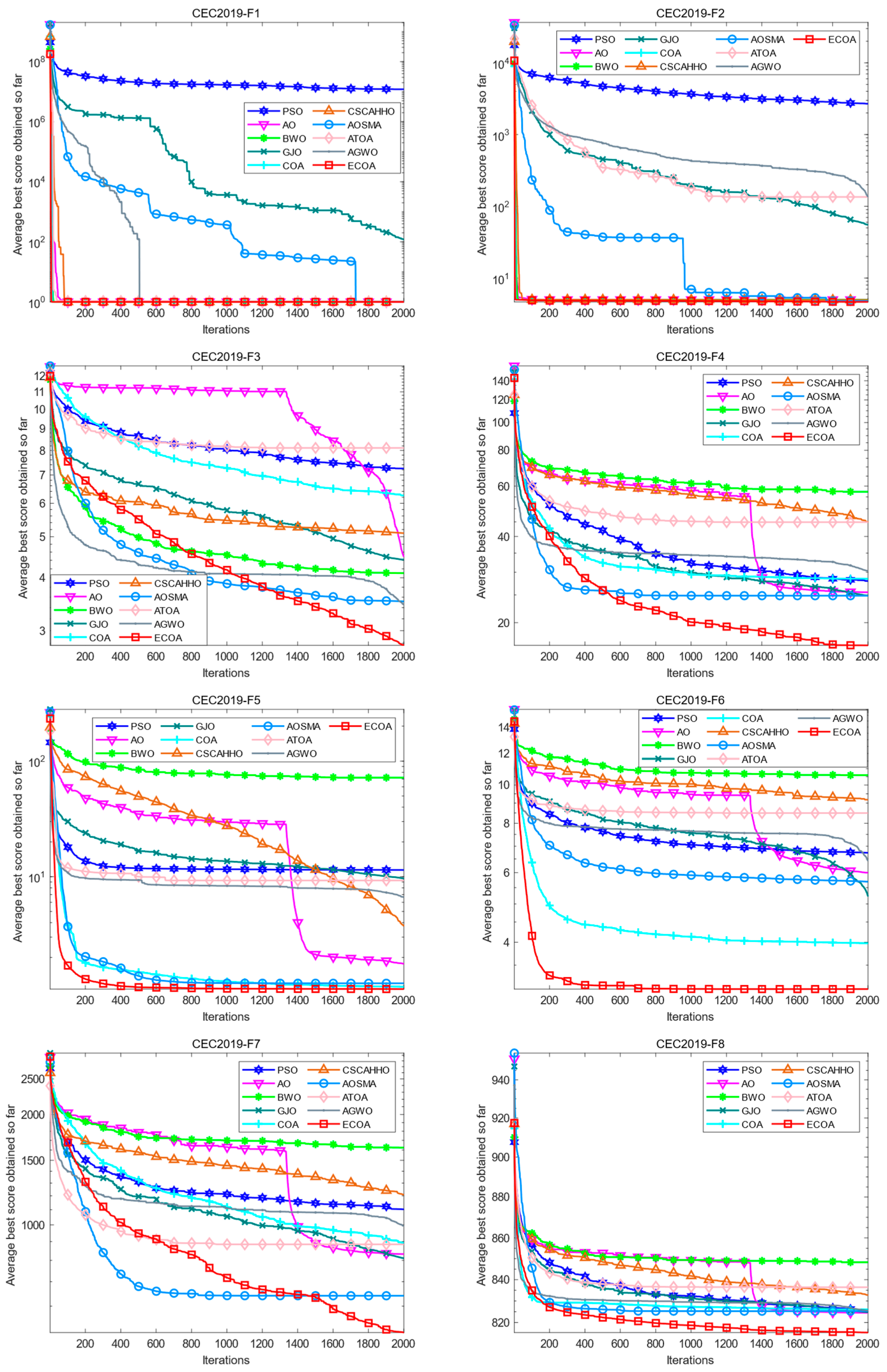
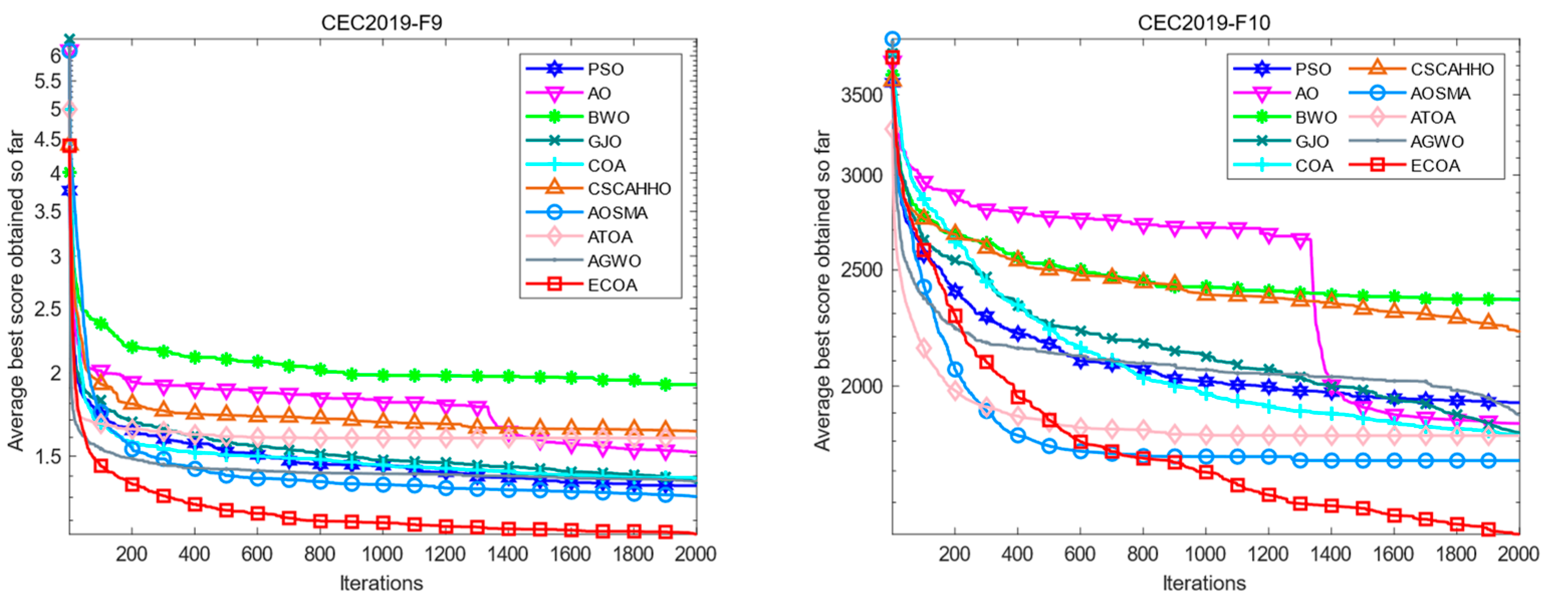
This paper took the average value of the 30 iterations in which each optimization algorithm was independently run and drew iteration curves for intuitive comparison to verify the proposed ECOA’s optimization performance further. The results are shown in Figure 2. On F1, in addition to the slow convergence speed of PSO and GJO, other algorithms converge quickly to the optimal value, and the ECOA’s convergence speed is the fastest. On F2, except for the slow convergence speed of PSO, GJO, ATOA, and AGWO, other algorithms converge to a quick and close precision. On F3, F4, F7, F8, F9, and F10, although the speed is slightly behind that of some algorithms in the early stage of iteration, other algorithms fall into local optimality with the progress of iteration. The speed is slower, while the ECOA can search and converge faster and has a more vital ability to jump out of local optimality. On both F5 and F6, the ECOA converges to a better value faster than other algorithms. The proposed ECOA has a faster convergence speed and a more vital ability to jump out of local optima compared with the standard optimization algorithm or improved algorithm.

4.4. Box Plot Analysis

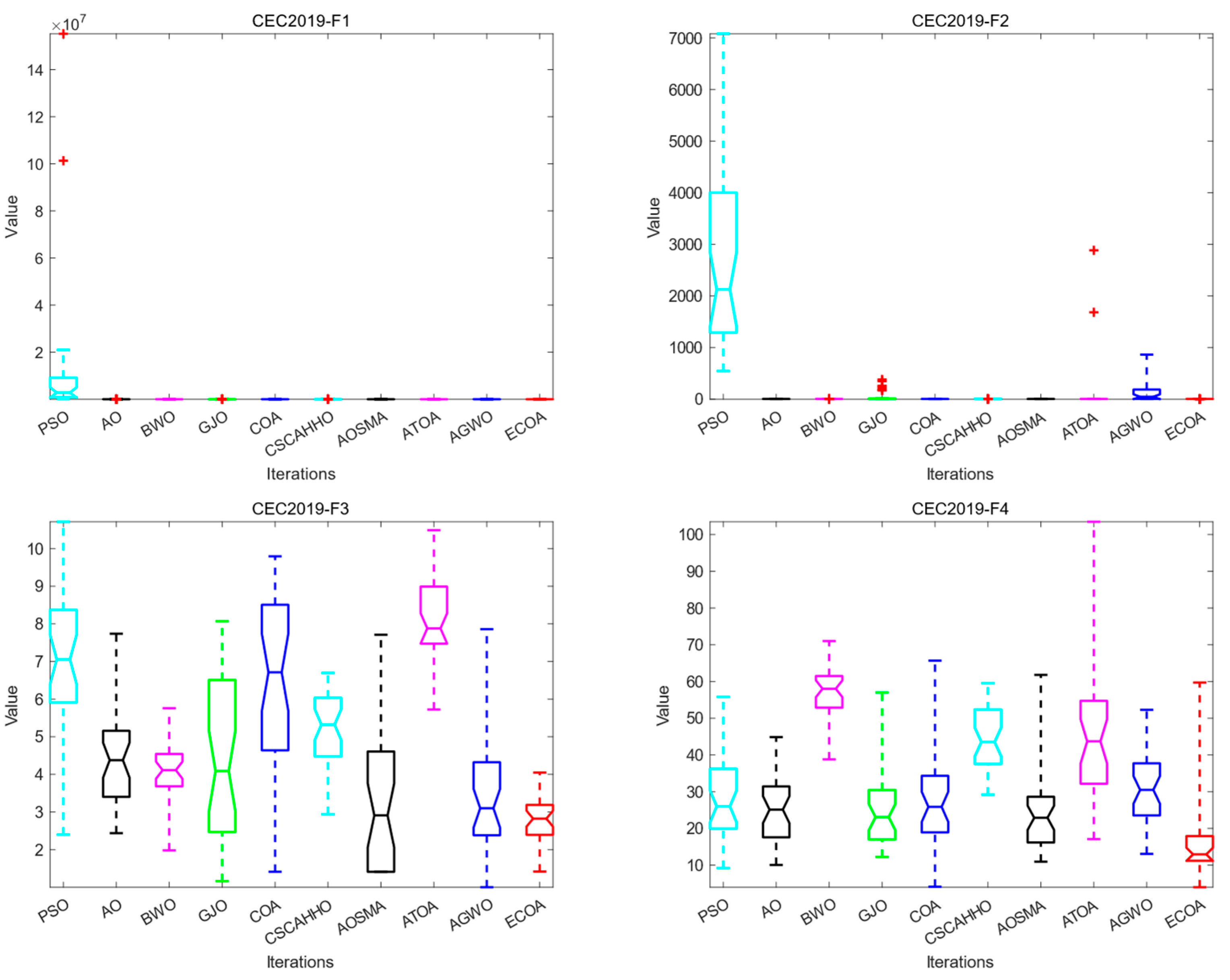
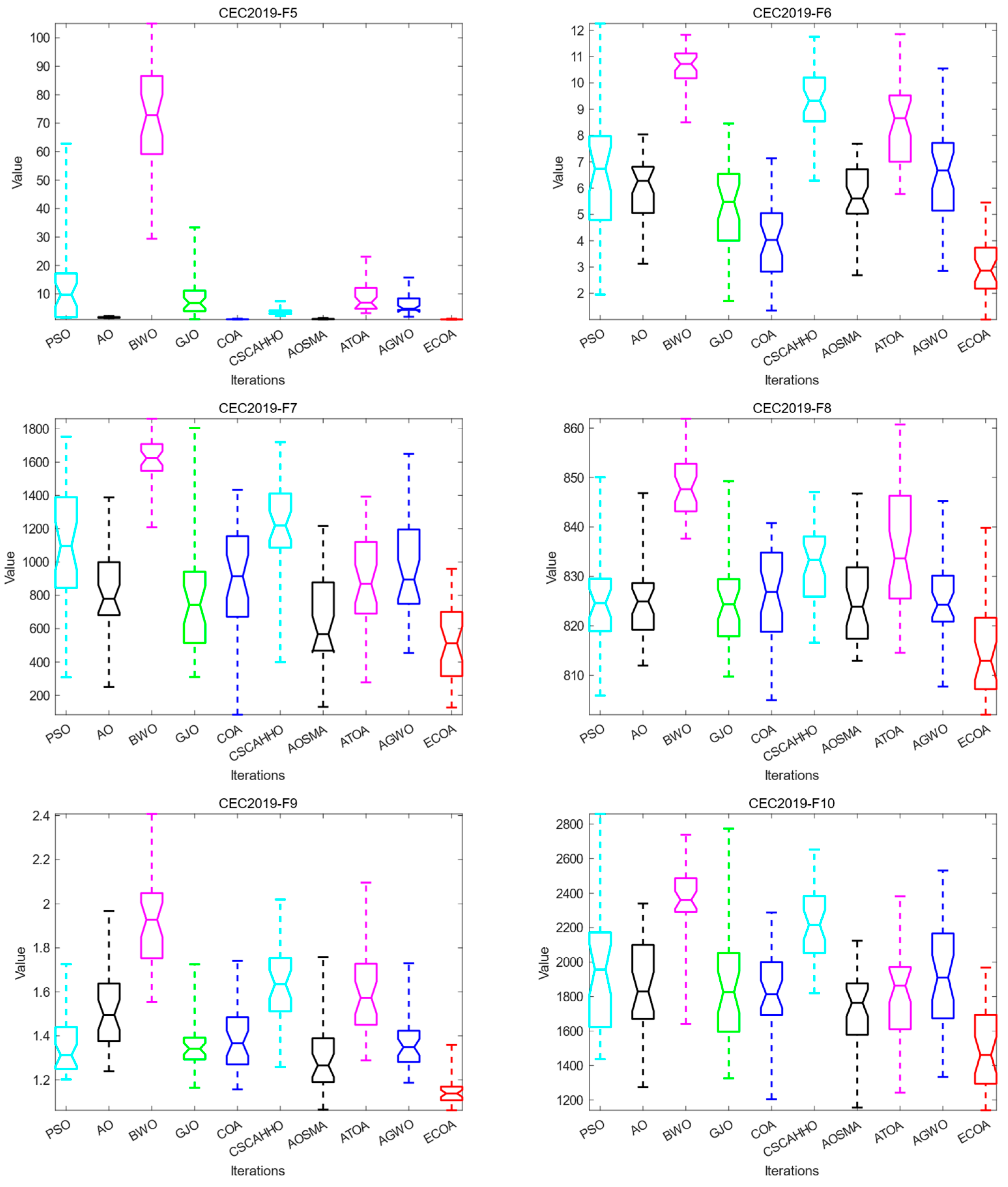
We draw boxplots according to the optimization results of the ECOA and other algorithms running 30 times on each test function and carry out the box plot analysis experiment. The boxplot [38] can reflect the distribution and spread range of 30 statistical results for each algorithm and reflect each algorithm’s performance stability when optimizing the IEEE CEC2019 test function. The shorter the box range means that the algorithm’s values are more similar when run several times, and the better the stability and reliability of the algorithm can be obtained. The smaller the value of the median line, the higher the optimization accuracy of the algorithm. The box diagram results are shown in Figure 3. In addition to the results of the ECOA boxplot on F1, F2, and F5, the ECOA’s boxplot range is shorter, and the median line is lower than that of the compared algorithms on other test functions. As a result, the ECOA can achieve better optimization results during multiple runs, and its performance is more stable, which can be used as a more reliable optimization algorithm.

4.5. The Wilcoxon Rank Sum Test

The Wilcoxon rank sum test [39] is a nonparametric statistical method that can statistically test the difference in the optimization performance of optimization algorithms. This paper compares the ECOA running 30 times in IEEE CEC2019 with the results of other algorithms by the Wilcoxon rank sum test. The p value of the significance level was set at 0.05. Suppose the rank sum test result of the ECOA and the compared algorithm is less than 0.05. In that case, it indicates that the optimization performance of the ECOA is completely better than that of the compared algorithm, and there is a significant difference. Table 4 shows the results of the Wilcoxon rank sum test between the ECOA and each algorithm. It can be seen that the p-value of the ECOA and the compared algorithm is less than 0.05 in most of the number functions, which has a significant difference. “N/A” indicates no significant difference between the two algorithms. In the last row of the table, the “worse”, “same”, and “better” of the optimization performance of the ECOA compared with the algorithm are visually counted, which are represented by “–”, “=“, and “+”, respectively. The performance of the ECOA in comparison to the compared algorithms is less than 0.05 in the vast majority of p-values, with slight differences only in individual functions (highlighted in bold). The rank sum test verifies that the ECOA has significantly improved performance compared with other algorithms.

4.6. Analysis of Ablation Experiments

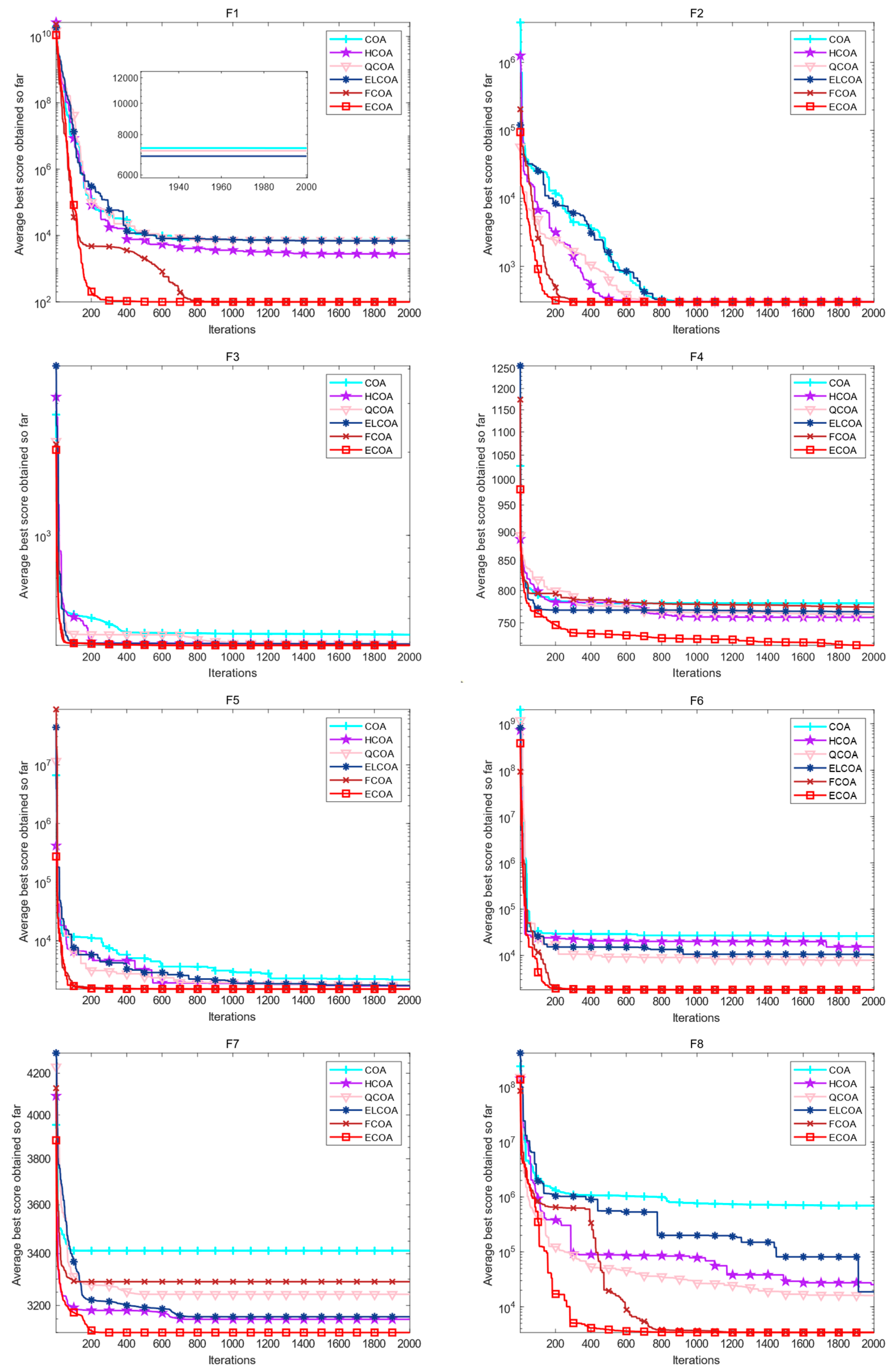
In this section, in order to further verify whether all four improvement strategies adopted for COA have had a positive improvement effect, ablation experiments are conducted to analyze. In the experiment, we will conduct ablation comparison experiments using only HCOA initialized with the Halton sequence, QCOA with only quasi opposition-based learning strategy, ELCOA with only elite factor, FCOA with only F A D s effect, original COA, and the ECOA proposed by the mixed four strategies. We selected eight different types of functions from the widely used and IEEE CEC2017 test function set for ablation experiments to further verify the rationality of the improved strategy and the superiority of the proposed ECOA. The information of eight test functions is shown in Table 5. To maintain fairness, the population size of all algorithms is set to 30 and the maximum number of iterations is set to 2000.
The iteration curve results of all algorithm ablation experiments are shown in Figure 4. The results show that on eight different types of IEEE CEC2017 test functions, each single strategy improved COA has faster convergence speed and optimization accuracy compared to the original algorithm, and the optimization performance of the proposed ECOA is significantly better than other algorithms. Through the above experiments, the feasibility of the adopted strategy was further verified, and mixing these four strategies can comprehensively improve the optimization performance of the original algorithm.

5. Practical Engineering Optimization Experiment

In this section, to verify the optimization performance of the proposed ECOA in solving practical engineering problems, we will use the ECOA to solve two engineering design optimization problems [40], namely the three-bar truss design problem and the pressure vessel design problem. Compared with other algorithms, 12 standard and improved algorithms were tested, including the marine predator algorithm (MPA), sine cosine algorithm [41] (SCA), PSO, AO, BWO, GJO, COA, CSCAHHO, AOSMA, ATOA, and AGWO. All algorithms run independently 30 times to statistically analyze the experimental results, with a population size of 30 and a maximum iteration count of 2000.

5.1. Three-Bar Truss Design Problem

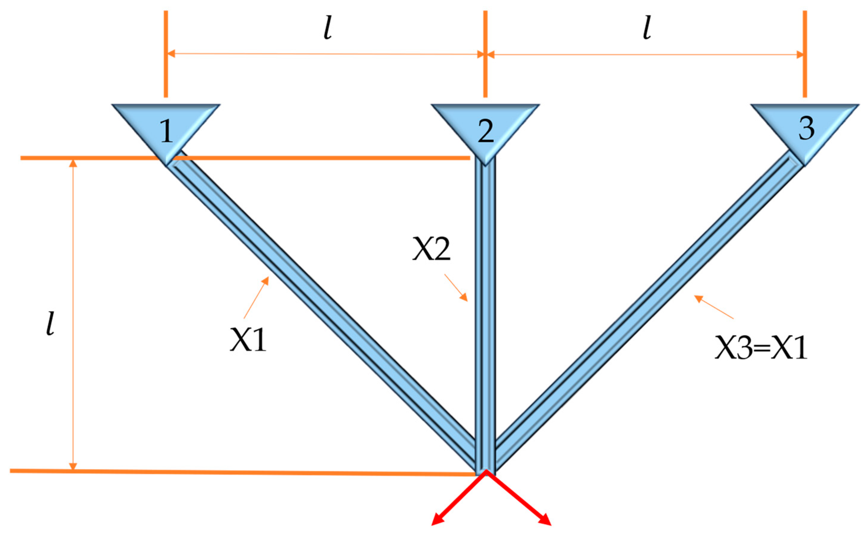
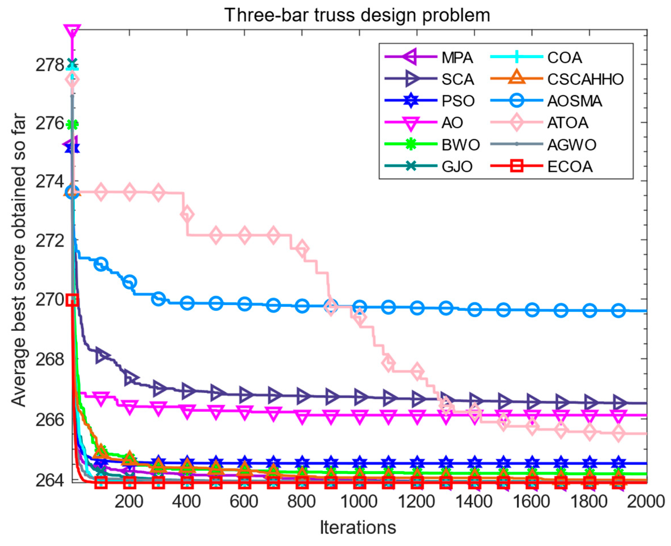
The three-bar truss design problem refers to the minimization of the volume of the truss by optimizing and adjusting the cross-sectional areas (X1 and X2) under stress constraints on each truss. The structure of the three-bar truss is shown in Figure 5, l represents spacing, X1, X2, and X3 represent cross-sectional areas. Its objective function is nonlinear and includes two decision parameters and three inequality constraints. The fitness iteration curve results of all algorithms are shown in Figure 6, which shows that compared to other algorithms, the ECOA has a faster convergence speed and higher convergence accuracy. The numerical results of each algorithm are summarized in Table 6. The ECOA results in higher accuracy and more stable performance.

5.2. Pressure Vessel Design

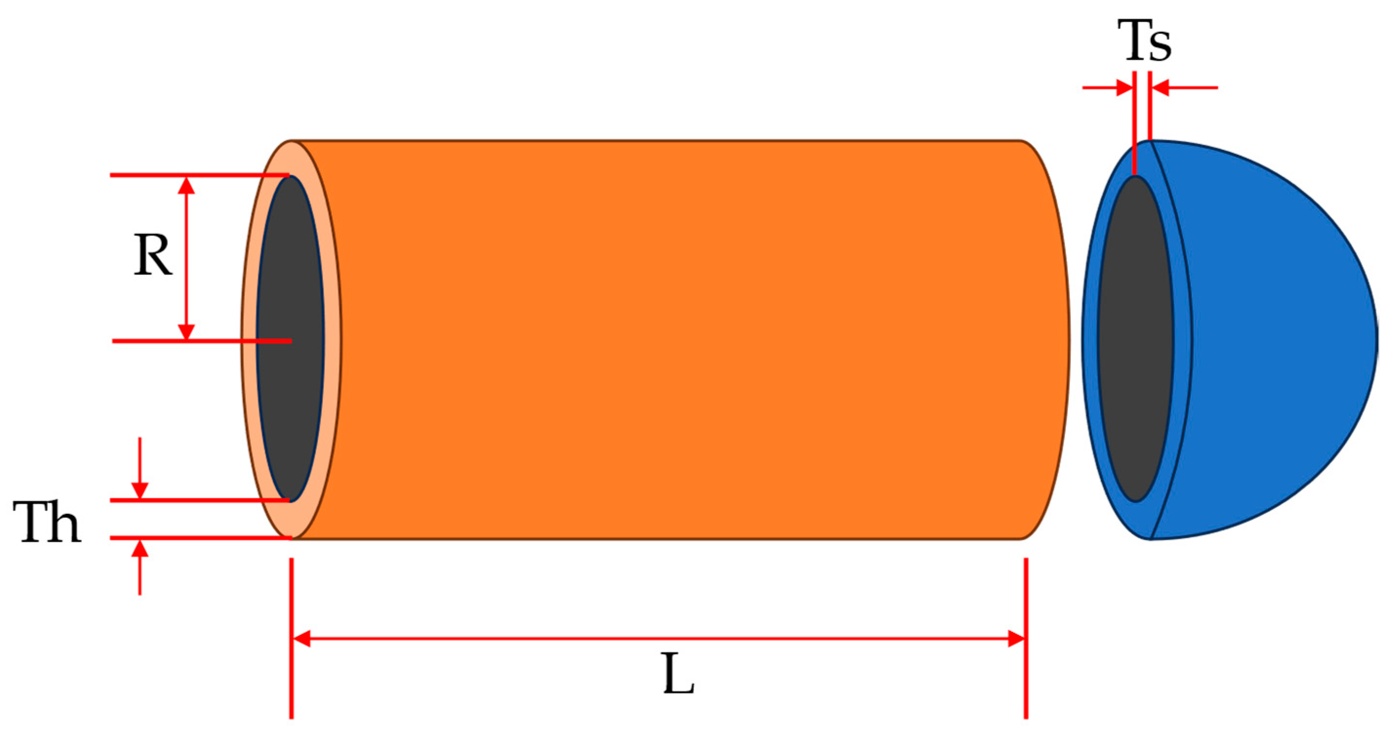
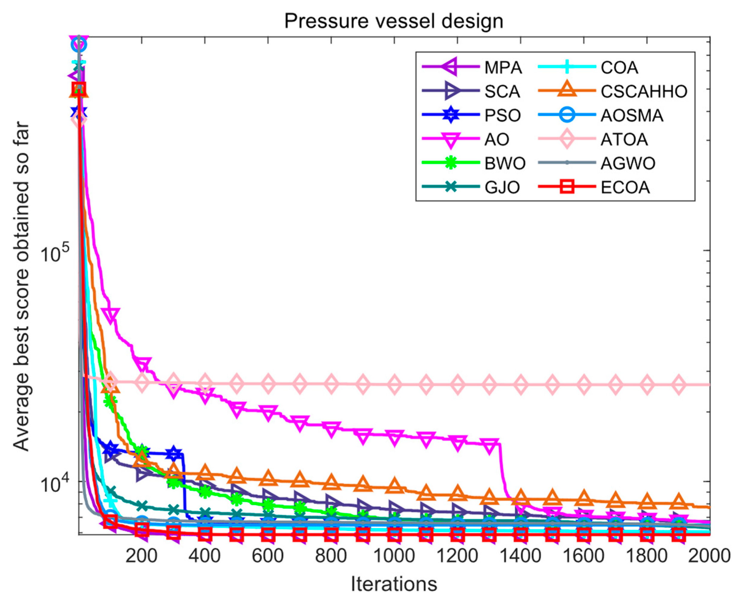
The pressure vessel design problem is to obtain the design structure of a pressure vessel with minimal cost through optimization while satisfying constraints. There are four decision variables that need to be optimized for this problem, namely: hemispherical head thickness (Th), container wall thickness (Ts), cylindrical section length (L), and inner diameter (R). The structural diagram of the pressure vessel is shown in Figure 7. The fitness iteration curves of all algorithms for pressure vessel design problems are shown in Figure 8. The optimization results of various algorithms for pressure vessel design problems are shown in Table 7. Based on the results in Figure 8 and Table 7, it can be seen that the results obtained by the ECOA and MPA are superior to those of other algorithms, and both have achieved optimal results. Moreover, from the convergence curve, it can be seen that the ECOA quickly converged to a better value, indicating its feasibility and superiority in applying to this problem.

6. Conclusions and Future Work

The crayfish optimization algorithm (COA) is a new swarm intelligence optimization algorithm that is performing well in global and engineering optimization. However, the COA also has some defects. In this paper, the standard COA mixing strategy is improved: (1) The Halton sequence is used to initialize the population so that the initial population is more evenly distributed in the search space, and the convergence speed of the initial COA iteration is increased. (2) QOBL is introduced to generate the quasi-oppositional solution of the population. The better solution is selected from the original solution, and the quasi-oppositional solution enters the next generation to improve the quality of candidate solutions. (3) Introducing elite guiding factors in the predation stage to avoid the blindness of this process. (4) The fish device aggregation effect (FADs) in the marine predator algorithm is introduced into COA to enhance its ability to jump out of local optimal. Based on the above, an enhanced crayfish optimization algorithm (ECOA) with better performance is proposed. This paper compares it with other optimization algorithms and improved algorithms on the CEC2019 test function and two real-world engineering optimization problems set to verify the effectiveness of the ECOA. The experimental results show that the ECOA can better balance the exploration and development of the algorithm and has a more robust global optimization ability. In future work, we will apply the ECOA to other practical problems, such as UAV track optimization, flexible shop scheduling, and microgrid optimization scheduling, to verify its ability to solve various complex practical problems.

Author Contributions

Conceptualization, Y.Z. and P.L.; methodology, Y.Z.; software, P.L.; validation, P.L. and Y.L.; formal analysis, Y.L.; writing—original draft preparation, Y.Z.; writing—review and editing, P.L.; visualization, Y.L. All authors have read and agreed to the published version of the manuscript.

Funding

This work is supported by the fund of the Science and Technology Development Project of Jilin Province No. 20220203190SF.

Data Availability Statement

The data that support the findings of this study are available from the corresponding author upon reasonable request.

Conflicts of Interest

The authors declare no conflict of interest.

References

  1. Hu, G.; Zhong, J.; Du, B.; Wei, G. An enhanced hybrid arithmetic optimization algorithm for engineering applications. Comput. Methods Appl. Mech. Eng. 2022, 394, 114901. [Google Scholar] [CrossRef]
  2. Jiang, Y.; Yin, S.; Dong, J.; Kaynak, O. A Review on Soft Sensors for Monitoring, Control, and Optimization of Industrial Processes. IEEE Sens. J. 2021, 21, 12868–12881. [Google Scholar] [CrossRef]
  3. Cosic, A.; Stadler, M.; Mansoor, M.; Zellinger, M. Mixed-integer linear programming based optimization strategies for renewable energy communities. Energy 2021, 237, 121559. [Google Scholar] [CrossRef]
  4. Shen, Y.; Branscomb, D. Orientation optimization in anisotropic materials using gradient descent method. Compos. Struct. 2020, 234, 111680. [Google Scholar] [CrossRef]
  5. Xu, Z.; Geng, H.; Chu, B. A Hierarchical Data–Driven Wind Farm Power Optimization Approach Using Stochastic Projected Simplex Method. IEEE Trans. Smart Grid 2021, 12, 3560–3569. [Google Scholar] [CrossRef]
  6. Mavrovouniotis, M.; Li, C.; Yang, S. A survey of swarm intelligence for dynamic optimization: Algorithms and applications. Swarm Evol. Comput. 2017, 33, 1–17. [Google Scholar] [CrossRef]
  7. Tang, J.; Liu, G.; Pan, Q. A Review on Representative Swarm Intelligence Algorithms for Solving Optimization Problems: Applications and Trends. IEEE/CAA J. Autom. Sin. 2021, 8, 1627–1643. [Google Scholar] [CrossRef]
  8. Li, W.; Wang, G.-G.; Gandomi, A.H. A Survey of Learning-Based Intelligent Optimization Algorithms. Arch. Comput. Methods Eng. 2021, 28, 3781–3799. [Google Scholar] [CrossRef]
  9. El-Kenawy, E.-S.M.; Khodadadi, N.; Mirjalili, S.; Abdelhamid, A.A.; Eid, M.M.; Ibrahim, A. Greylag Goose Optimization: Nature-inspired optimization algorithm. Expert Syst. Appl. 2024, 238, 122147. [Google Scholar] [CrossRef]
  10. Dorigo, M.; Birattari, M.; Stutzle, T. Ant colony optimizationtimization. IEEE Comput. Intell. Mag. 2006, 1, 28–39. [Google Scholar] [CrossRef]
  11. Kennedy, J.; Eberhart, R. Particle swarm optimization. In Proceedings of the ICNN’95—International Conference on Neural Networks, Perth, WA, Australia, 27 November–1 December 1995; Volume 4, pp. 1942–1948. [Google Scholar] [CrossRef]
  12. Mirjalili, S.; Lewis, A. The Whale Optimization Algorithm. Adv. Eng. Softw. 2016, 95, 51–67. [Google Scholar] [CrossRef]
  13. Elseify, M.A.; Hashim, F.A.; Hussien, A.G.; Kamel, S. Single and multi-objectives based on an improved golden jackal optimization algorithm for simultaneous integration of multiple capacitors and multi-type DGs in distribution systems. Appl. Energy 2024, 353, 122054. [Google Scholar] [CrossRef]
  14. Moazen, H.; Molaei, S.; Farzinvash, L.; Sabaei, M. PSO-ELPM: PSO with elite learning, enhanced parameter updating, and exponential mutation operator. Inf. Sci. 2023, 628, 70–91. [Google Scholar] [CrossRef]
  15. Shen, Y.; Zhang, C.; Gharehchopogh, F.S.; Mirjalili, S. An improved whale optimization algorithm based on multi-population evolution for global optimization and engineering design problems. Expert Syst. Appl. 2023, 215, 119269. [Google Scholar] [CrossRef]
  16. Zhu, F.; Li, G.; Tang, H.; Li, Y.; Lv, X.; Wang, X. Dung beetle optimization algorithm based on quantum computing and multi-strategy fusion for solving engineering problems. Expert Syst. Appl. 2024, 236, 121219. [Google Scholar] [CrossRef]
  17. Zhang, X.; Sang, H.; Li, Z.; Zhang, B.; Meng, L. An efficient discrete artificial bee colony algorithm with dynamic calculation method for solving the AGV scheduling problem of delivery and pickup. Complex Intell. Syst. 2024, 10, 37–57. [Google Scholar] [CrossRef]
  18. Yang, Y.; Qiu, J.; Qin, Z. Multidimensional Firefly Algorithm for Solving Day-Ahead Scheduling Optimization in Microgrid. J. Electr. Eng. Technol. 2021, 16, 1755–1768. [Google Scholar] [CrossRef]
  19. Song, Q.; Zhao, Q.; Wang, S.; Liu, Q.; Chen, X. Dynamic Path Planning for Unmanned Vehicles Based on Fuzzy Logic and Improved Ant Colony Optimization. IEEE Access 2020, 8, 62107–62115. [Google Scholar] [CrossRef]
  20. Kalita, K.; Ramesh, J.V.N.; Cepova, L.; Pandya, S.B.; Jangir, P.; Abualigah, L. Multi-objective exponential distribution optimizer (MOEDO): A novel math-inspired multi-objective algorithm for global optimization and real-world engineering design problems. Sci. Rep. 2024, 14, 1816. [Google Scholar] [CrossRef]
  21. Al Aghbari, Z.; Raj, P.V.P.; Mostafa, R.R.; Khedr, A.M. iCapS-MS: An improved Capuchin Search Algorithm-based mobile-sink sojourn location optimization and datdata collection scheme for Wireless Sensor Networks. Neural Comput. Appl. 2024, 36, 8501–8517. [Google Scholar] [CrossRef]
  22. Jia, H.; Rao, H.; Wen, C.; Mirjalili, S. Crayfish optimization algorithm. Artif. Intell. Rev. 2023, 56 (Suppl. S2), 1919–1979. [Google Scholar] [CrossRef]
  23. Li, Q.; Liu, S.-Y.; Yang, X.-S. Influence of initialization on the performance of metaheuristic optimizers. Appl. Soft Comput. 2020, 91, 106193. [Google Scholar] [CrossRef]
  24. Wei, F.; Zhang, Y.; Li, J. Multi-strategy-based adaptive sine cosine algorithm for engineering optimization problems. Expert Syst. Appl. 2024, 248, 123444. [Google Scholar] [CrossRef]
  25. Halton, J.H. Algorithm 247: Radical-inverse quasi-random point sequence. Commun. ACM 1964, 7, 701–702. [Google Scholar] [CrossRef]
  26. Tizhoosh, H.R. Opposition-Based Learning: A New Scheme for Machine Intelligence. In Proceedings of the International Conference on Computational Intelligence for Modelling, Control and Automation and International Conference on Intelligent Agents, Web Technologies and Internet Commerce (CIMCA-IAWTIC’06), Vienna, Austria, 28–30 November 2005; pp. 695–701. [Google Scholar] [CrossRef]
  27. Truonga, K.H.; Nallagownden, P.; Baharudin, Z.; Vo, D.N. A Quasi-Oppositional-Chaotic Symbiotic Organisms Search algorithm for global optimization problems. Appl. Soft Comput. 2019, 77, 567–583. [Google Scholar] [CrossRef]
  28. Yang, X.; Hao, X.; Yang, T.; Li, Y.; Zhang, Y.; Wang, J. Elite-guided multi-objective cuckoo search algorithm based on crossover operation and information enhancement. Soft Comput. 2023, 27, 4761–4778. [Google Scholar] [CrossRef]
  29. Faramarzi, A.; Heidarinejad, M.; Mirjalili, S.; Gandomi, A.H. Marine Predators Algorithm: A nature-inspired metaheuristic. Expert Syst. Appl. 2020, 152, 113377. [Google Scholar] [CrossRef]
  30. Zhang, M.; Tan, K.C. Conference Report on 2019 IEEE Congress on Evolutionary Computation (IEEE CEC 2019). IEEE Comput. Comput. Intell. Mag. 2020, 15, 4–5. [Google Scholar] [CrossRef]
  31. Abualigah, L.; Yousri, D.; Elaziz, M.A.; Ewees, A.A.; Al-Qaness, M.A.A.; Gandomi, A.H. Aquila Optimizer: A novel meta-heuristic optimization algorithm. Comput. Ind. Eng. 2021, 157, 107250. [Google Scholar] [CrossRef]
  32. Zhong, C.; Li, G.; Meng, Z. Beluga whale optimization: A novel nature-inspired metaheuristic algorithm. Knowl. -Based Syst. 2022, 251, 109215. [Google Scholar] [CrossRef]
  33. Chopra, N.; Ansari, M.M. Golden jackal optimization: A novel nature-inspired optimizer for engineering applications. Expert Syst. Appl. 2022, 198, 116924. [Google Scholar] [CrossRef]
  34. Zhang, Y.-J.; Yan, Y.-X.; Zhao, J.; Gao, Z.-M. CSCAHHO: Chaotic hybridization algorithm of the Sine Cosine with Harris Hawk optimization algorithms for solving global optimization problems. PLoS ONE 2022, 17, e0263387. [Google Scholar] [CrossRef]
  35. Naik, M.K.; Panda, R.; Abraham, A. Adaptive opposition slime mould algorithm. Soft Comput. 2021, 25, 14297–14313. [Google Scholar] [CrossRef]
  36. Devan, P.A.M.; Hussin, F.A.; Ibrahim, R.B.; Bingi, K.; Nagarajapandian, M.; Assaad, M. An Arithmetic-Trigonometric Optimization Algorithm with Application for Control of Real-Time Pressure Process Plant. Sensors 2022, 22, 617. [Google Scholar] [CrossRef]
  37. Meidani, K.; Hemmasian, A.; Mirjalili, S.; Farimani, A.B. Adaptive grey wolf optimizer. Neural Comput. Appl. 2022, 34, 7711–7731. [Google Scholar] [CrossRef]
  38. Streit, M.; Gehlenborg, N. Bar charts and box plots. Nat. Methods 2014, 11, 117. [Google Scholar] [CrossRef]
  39. Bo, Q.; Cheng, W.; Khishe, M. Evolving chimp optimization algorithm by weighted opposition-based technique and greedy search for multimodal engineering problems. Appl. Soft Comput. 2023, 132, 109869. [Google Scholar] [CrossRef]
  40. Zhang, S.-W.; Wang, J.-S.; Li, Y.-X.; Zhang, S.-H.; Wang, Y.-C.; Wang, X.-T. Improved honey badger algorithm based on elementary function density factors and mathematical spirals in polar coordinate systema. Artif. Intell. Rev. 2024, 57, 55. [Google Scholar] [CrossRef]
  41. Mirjalili, S. SCA: A Sine Cosine Algorithm for solving optimization problems. Knowl.-Based Syst. 2016, 96, 120–133. [Google Scholar] [CrossRef]
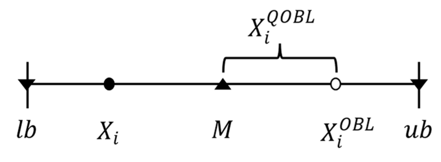
Figure 1. Schematic diagram of individual location of QOBL population.
Biomimetics 09 00341 g001
Figure 2. Comparison of iteration curves of each algorithm on the CEC2019 test set.
Biomimetics 09 00341 g002aBiomimetics 09 00341 g002b
Figure 3. Comparison of box plots of various algorithms on the CEC2019 test set.
Biomimetics 09 00341 g003aBiomimetics 09 00341 g003b
Figure 4. Iteration curves of various algorithms in ablation experiments.
Biomimetics 09 00341 g004
Figure 5. Three-bar truss structure diagram.
Biomimetics 09 00341 g005
Figure 6. Iterative curves of various algorithms for three-bar truss design problems.
Biomimetics 09 00341 g006
Figure 7. Schematic diagram of pressure vessel structure.
Biomimetics 09 00341 g007
Figure 8. Iterative curves of various algorithms for pressure vessel design.
Biomimetics 09 00341 g008
Table 1. Information of IEEE CEC2019 test function set.
FunctionName D Search RangeOptimum
F1Storn’s Chebyshev Polynomial Fitting Problem9[−8192, 8192]1
F2Inverse Hilbert Matrix Problem16[−16,384, 16,384]1
F3Lennard–Jones Minimum Energy Cluster18[−4, 4]1
F4Rastrigin’s Function10[−100, 100]1
F5Griewangk’s Function10[−100, 100]1
F6Weierstrass Function10[−100, 100]1
F7Modified Schwefel’s Function10[−100, 100]1
F8Expanded Schaffer’s F6 Function10[−100, 100]1
F9Happy Cat Function10[−100, 100]1
F10Ackley Function10[−100, 100]1
Table 2. Important parameter settings of each algorithm.
AlgorithmsParameters
PSO ω   = 0.9, C1 = C2 = 2
AO α   = 0.1 ,   δ   = 0.1
BWOProbability of whale fall decreased at interval W f [ 0.1 ,   0.05 ]
GJO E 0 [ 1 ,   1 ]
COA r [ 0 ,   1 ] ,   C 2 = 2 t / T ,   C 3 = 3 ,
CSCAHHO a = 2 ,   r ,     r 1 [ 0 ,   1 ] ,   r 2 [ 0 ,   2 π ] , r 3 [ 0 ,   2 ] ,   E 1 [ 2 ,   0 ]
AOSMA δ = 0.03
ATOA min = 0.2 ,   max = 1 ,   α = 5 ,   μ = 0.499 ,   ε = 1
AGWO γ damping when F is not decreasing significantly
ECOA F A D s   = 0.2
Table 3. Numerical experimental results of each algorithm on the CEC2019 test set.
CEC2019ValuePSOAOBWOGJOCOACSCAHHOAOSMAATOAAGWOECOA
F1Best1.361 × 10+5111111111
Mean1.202 × 10+711120.2597111111
Std3.027 × 10+71.135 × 10−90642.78809.879 × 10−110000
F2Best545.919254.85564.21974.05574.27394.23164.47554.21743.2141
Mean2689.105554.993555.31574.80874.94494.7893135.0859133.8714.6568
Std1741.300100.027086106.43490.333740.173280.32882556.0031194.26980.64381
F3Best2.39792.43611.98051.16341.41042.94111.40915.72341.00041.4173
Mean7.25014.48844.1034.41366.26065.09943.5178.10863.4622.7698
Std1.96161.28680.7662.28712.66031.07522.22991.22771.5320.62451
F4Best9.220910.057638.800912.2484.141429.190110.949617.089813.06033.9849
Mean27.944625.534257.315324.84328.439744.821724.839344.880930.326416.6629
Std11.07348.79016.936510.742815.74638.859111.323116.76329.523811.1345
F5Best1.55111.483329.4051.13391.04972.19181.02463.26751.96981.0074
Mean11.4281.759772.02119.55421.1153.72371.1949.27336.63921.0641
Std13.50640.1866319.47829.01790.0613051.12330.116465.83613.80980.050987
F6Best1.95523.12148.50151.70381.34436.28462.68725.77682.85081.0041
Mean6.73675.998210.59025.22583.97849.17075.69188.49216.42513.0444
Std2.45931.24840.778041.72371.54531.33841.30331.61491.75361.268
F7Best308.3668249.34341208.3006309.912283.4932399.241130.7135278.2579453.8124126.6386
Mean1102.4747832.30151623.6728810.9943894.6441206.1076640.6508884.6521994.0343508.5085
Std355.712265.7038130.0862376.0119339.8851290.3894277.6008269.8459298.1859230.6677
F8Best805.925811.9902837.6275809.7835804.9748816.6299812.9345814.5553807.7328802.0457
Mean825.7583824.5015848.2828824.7693825.9996832.6092825.2471836.4446825.521815.3867
Std10.10057.47536.02629.25268.94548.43708.926313.11827.85719.9757
F9Best1.16161.15321.54751.20251.16831.35141.05381.19771.21291.0359
Mean1.35791.49241.93411.32281.37861.65911.28421.60301.39561.1378
Std0.09990.16970.13360.09280.14420.15450.12230.22050.11290.0522
F10Best1436.991274.081641.751325.811204.191818.691155.341241.951333.241139.99
Mean1937.941861.892362.491828.641819.192217.231733.811819.031892.9621505.39
Std349.35275.94194.21344.89267.68216.92214.91268.69309.42229.69
Table 4. Test p-values of each algorithm on the IEEE CEC2019 test set.
CEC2019PSOAOBWOGJOCOACSCAHHOAOSMAATOAAGWO
F11.534 × 10−143.706 × 10⁻⁴N/A1.534 × 10−14N/A2.527 × 10−10N/AN/AN/A
F21.322 × 10−133.017 × 10−33.031 × 10−32.943 × 10−27.786 × 10−13.253 × 10−19.044 × 10−18.363 × 10−21.162 × 10−7
F35.851 × 10−122.255 × 10−82.789 × 10−97.939 × 10−32.678 × 10−71.438 × 10−118.325 × 10−16.545 × 10−135.119 × 10⁻²
F46.466 × 10−67.221 × 10−63.865 × 10−126.834 × 10−56.189 × 10−59.661 × 10−117.922 × 10−52.254 × 10−101.955 × 10⁻⁷
F56.545 × 10−136.545 × 10−136.545 × 10−137.132 × 10−132.477 × 10−56.545 × 10−132.248 × 10−96.545 × 10−136.545 × 10⁻¹³
F64.928 × 10−92.625 × 10−106.545 × 10−131.156 × 10−61.044 × 10−26.545 × 10−131.565 × 10−96.545 × 10−132.625 × 10⁻¹⁰
F77.510 × 10−106.118 × 10−66.545 × 10−135.536 × 10−42.204 × 10−62.527 × 10−116.689 × 10−24.399 × 10−71.307 × 10⁻⁸
F81.413 × 10−49.620 × 10−57.761 × 10−132.363 × 10−42.608 × 10−51.399 × 10−85.327 × 10−58.626 × 10−93.935 × 10−5
F95.851 × 10−122.342 × 10−126.545 × 10−134.566 × 10−125.388 × 10−126.545 × 10−132.761 × 10−81.191 × 10−121.411 × 10⁻¹²
F105.620 × 10−71.852 × 10−61.819 × 10−124.357 × 10−54.628 × 10−62.342 × 10−121.348 × 10−49.498 × 10−61.090 × 10⁻⁶
−/=/+0/0/100/0/100/1/90/0/100/2/80/1/90/4/60/2/80/2/8
Table 5. Information on the eight test functions of IEEE CEC2017.
Function TypeFunction NumberNameDimensionTheoretical Optimal Value
Unimodal functionCEC2017-F1Shifted and rotated bent cigar function10100
CEC2017-F2Shifted and rotated zakharov function10300
Multimodal functionCEC2017-F3Shifted and rotated Rosenbrock’s function10400
CEC2017-F4Shifted and rotated lunacek Bi_Rastrigin10700
Hybrid functionCEC2017-F5Hybrid function 5 (N = 4)101500
CEC2017-F6Hybrid function 6 (N = 5)101800
Composition functionCEC2017-F7Composition function 8 (N = 6)102800
CEC2017-F8Composition function 10 (N = 3)103000
Table 6. Experimental results of various algorithms on the three-bar truss design problems.
AlgorithmsDecision VariablesBestMeanStd
X1X2
MPA0.7885436610.408621746263.8958263.89602.2142 × 10−4
SCA0.8170875690.354123484263.9162266.51966.5123
PSO0.7956456560.394874029263.8959264.53003.4587
AO0.7591974790.513909988264.0598266.12452.0766
BWO0.7893219150.409324881263.8969264.18640.2262
GJO0.7895079170.405951715263.8961263.90170.0048061
COA0.7886047060.408449023263.8959263.89601.3825 × 10−4
CSCAHHO0.7908608570.402928576263.8959263.98210.11688
AOSMA0.7358181170.614832778264.1893269.60412.1968
ATOA0.8221923050.329610280263.9000265.51212.2217
AGWO0.7888288450.407890221263.8972263.90350.0067363
ECOA0.7886751350.408248289263.8958263.89581.7345 × 10−13
Table 7. Experimental results of various algorithms in pressure vessel design.
AlgorithmsDecision VariablesBestMeanStd
ThTsLR
MPA0.3846491630.77816864120040.319618725885.33285885.33285.3255 × 10−13
SCA0.4992918800.925842231146.404885146.382430535984.18736717.5887563.3545
PSO0.4853681910.971227746119.834881350.227480555887.88886471.8242667.9827
AO0.5079636541.000199547101.894160651.190450016099.87676649.8309433.1601
BWO0.4755368710.888263455155.189621744.843733265936.49476469.8463340.4535
GJO0.4612828960.928624719132.50474548.08930525890.14956298.0075527.7598
COA0.422041870.846150966161.182389343.806030795886.77756050.5243202.9679
CSCAHHO0.6094163811.23675193346.2575411859.248403476085.66217694.8483900.2840
AOSMA0.4920610060.995469322103.786004751.578721335890.49976475.3967587.2016
ATOA0.8659033311.88567638451.1029264484.144504316843.704426,244.236526,733.8240
AGWO0.4733620910.950451055124.834230149.176786645895.67726376.1675567.2517
ECOA0.3846491630.77816864120040.319618725885.33285885.33281.6889 × 10−13
Disclaimer/Publisher’s Note: The statements, opinions and data contained in all publications are solely those of the individual author(s) and contributor(s) and not of MDPI and/or the editor(s). MDPI and/or the editor(s) disclaim responsibility for any injury to people or property resulting from any ideas, methods, instructions or products referred to in the content.