


Bio-Inspired Space Robotic Control Compared to Alternatives


Abstract
1. Introduction
1.1. Broad Context and Why This Study Is Important
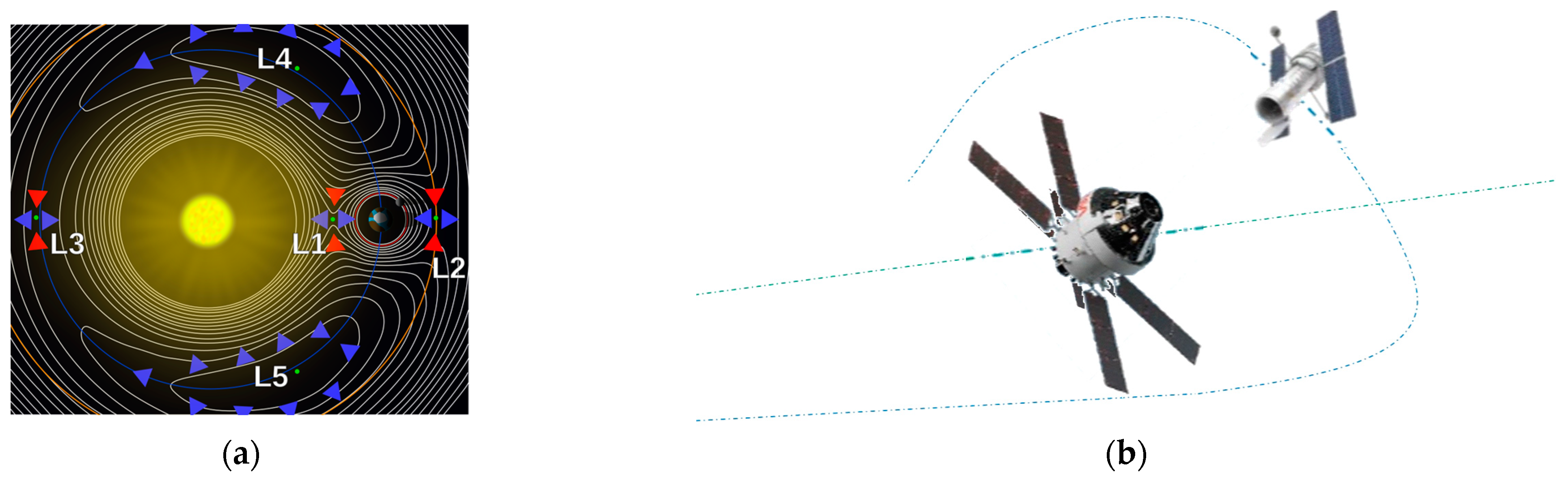
1.1.1. Cislunar Space
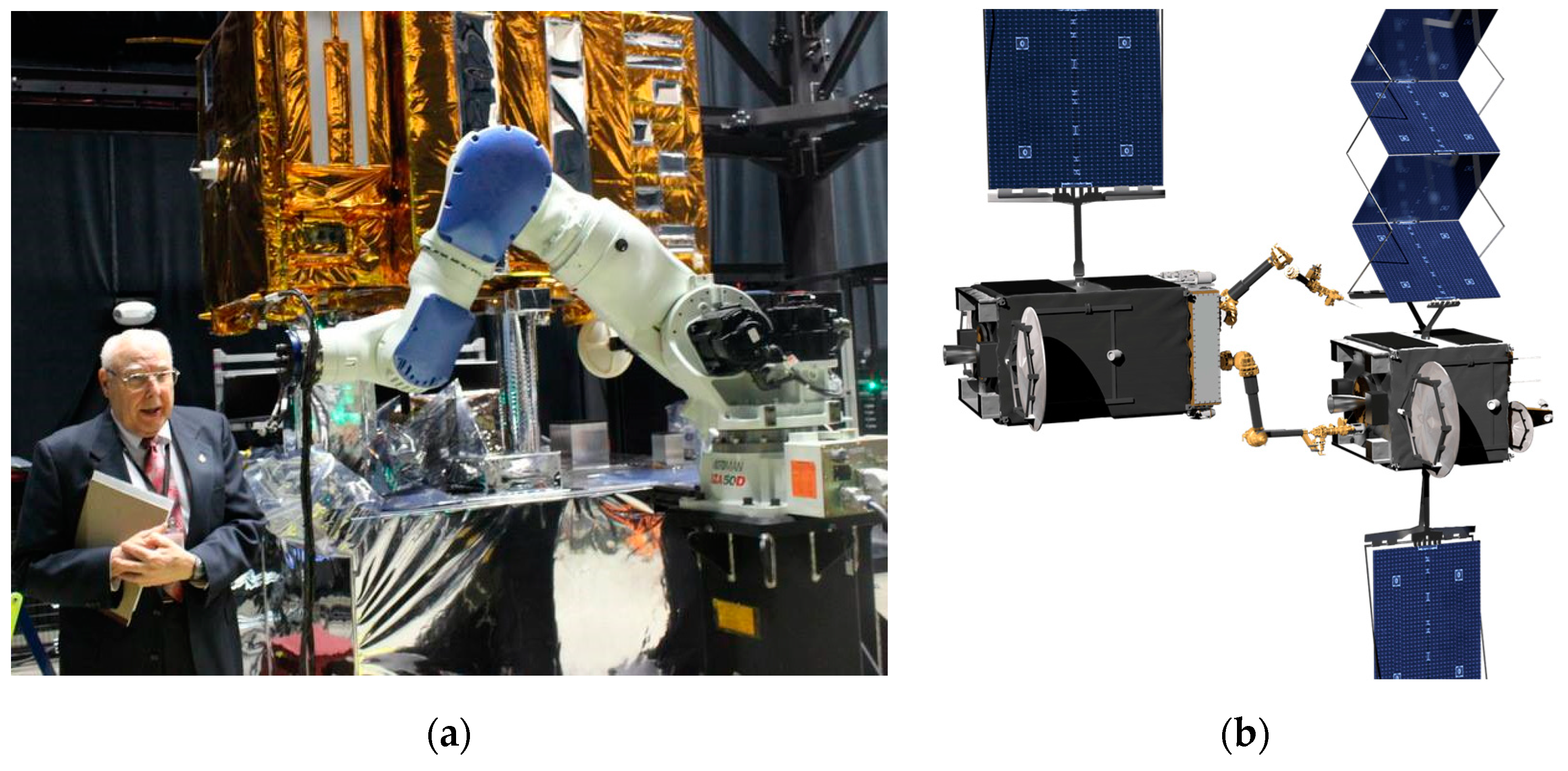
1.1.2. Cislunar Robotic Operations

| Variable/Acronym | Definition | Variable/Acronym | Definition |
|---|---|---|---|
| Centerline unit vector | Appendage stiffness | ||
| Control torque | Flexible masses and inertias | ||
| Main body inertia mass moment | Flexible inertia mass moment | ||
| Main body rotation angle | Translation and rotation angles |

1.2. Broad Review of Modeling and Control from First Principles to Modern Instantiations
1.3. The Current State of the Research Field and Key References
- Gain stabilization [56]: Tuning of gain to achieve stability of the rigid-body mode. Advantages: simplicity and based on well-known mathematics. Disadvantages: imprecise and uses effort (or equivalently fuel) wastefully compared to more modern methods.
- Classical second-order structural filtering [56]: Second-order filters designed for each chosen resonance and anti-resonance, usually of the lowest mode or the lowest two modes to ensure stability. Advantages: aids fuel usage of gain stabilization approaches. Disadvantages: mathematic model must have precision and remain not time varying.
- Rigid-body, minimum-fuel input trajectory shaping: Apply control analytically derived from constrained control-minimization boundary value problem solutions. Advantages: existing proofs of mathematical optimality. Disadvantages: lacks robustness.
- Single-frequency trajectory shaping: The fashion commanded trajectory from a single sinusoid chosen to avoid mode frequencies of the flexible robot. Advantages: simplicity. Disadvantages: still need accurate mathematical models to properly pick the single frequency.
- Flatten the curve to improve stability: Use option #2 to compensate for all structural modes seeking to create a magnitude response curve resembling such a curve for a second-order rigid-body system (primary motivation remains increased system stability). Advantages: aids fuel usage of gain stabilization approaches. Disadvantages: mathematic model must have precision and remain not time varying.
- Flatten the curve to improve trajectory tracking: This option is like option #7, except choosing parts of modes (resonance or anti-resonance) to minimize trajectory tracking errors (proposed in this manuscript). Advantages: aids fuel usage of gain stabilization approaches. Disadvantages: mathematic model must have precision and remain not time varying.
- Deterministic artificial intelligence: Use physics to define robot self-awareness, while adapting or learning time-varying physical system parameters (e.g., mass, mass moments, stiffness, and damping). Advantages: proofs of optimality, robustness and simple algorithms. Disadvantages: relatively unknown compared to peer methods.
- 9.1
- Self-awareness statements [62]: Use governing equations from physics to exclusively define robot self-awareness, while prescribing necessary trajectories to be tracked (currently only sinusoidal trajectories and control-minimizing trajectories are in the literature).
- 9.2
1.4. Controversial and Diverging Hypotheses—Literature Gaps
1.5. Main Aim of the Work and Highlighting of Principal Conclusions
1.6. Novelties Presented
- Commanded trajectory-shaping options are compared using control effort and tracking accuracy, and recommendations are offered.
- Feedforward controls are compared using control effort and tracking accuracy, and recommendations are offered.
- Commanded trajectories are compared with filtered feedback and no feedforward using least control effort tracking accuracy, and recommendations are offered.
- Mode 1 filtering options are compared using control effort tracking accuracy, and recommendations are offered.
- Mode 3 filtering options are compared using control effort tracking accuracy, and recommendations are offered.
- Mode 4 filtering options are compared using control effort tracking accuracy, and recommendations are offered.
- Overall recommendations are made for selection of commanded trajectories, feedforward controls, and filtered versus unfiltered feedback.
- The least control effort was achieved with step trajectories, rigid-body optimal feedforward control and unfiltered feedback, while recommendations are offered based on tracking accuracy and control effort.
2. Materials and Methods
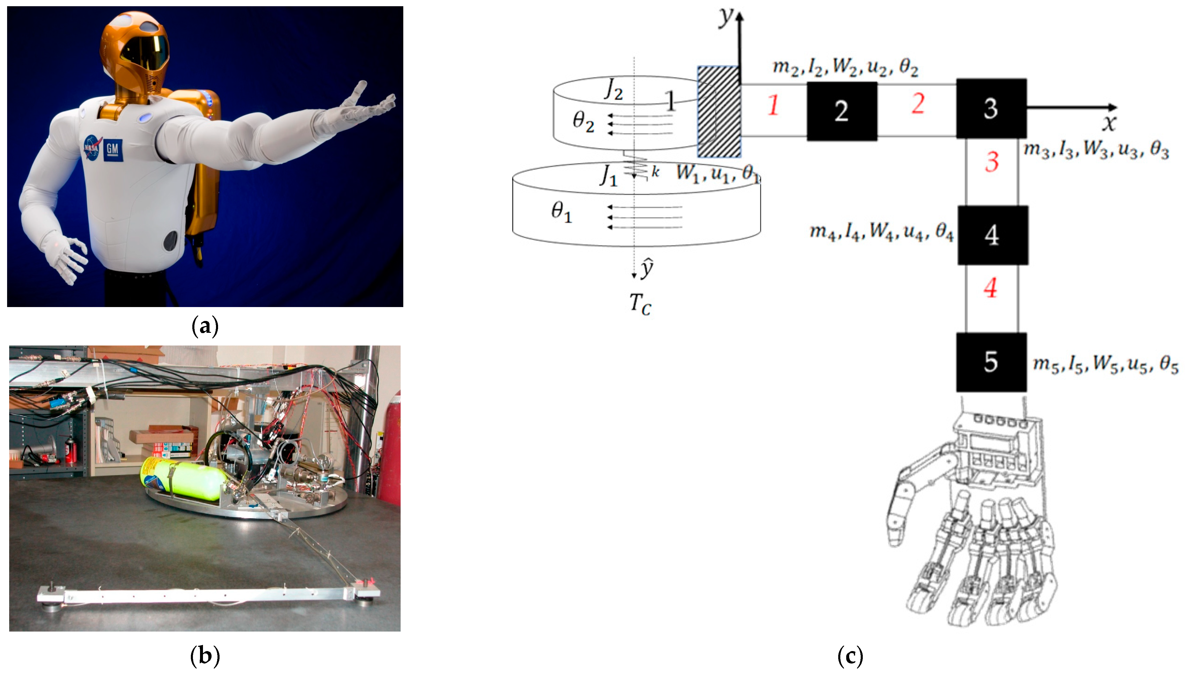
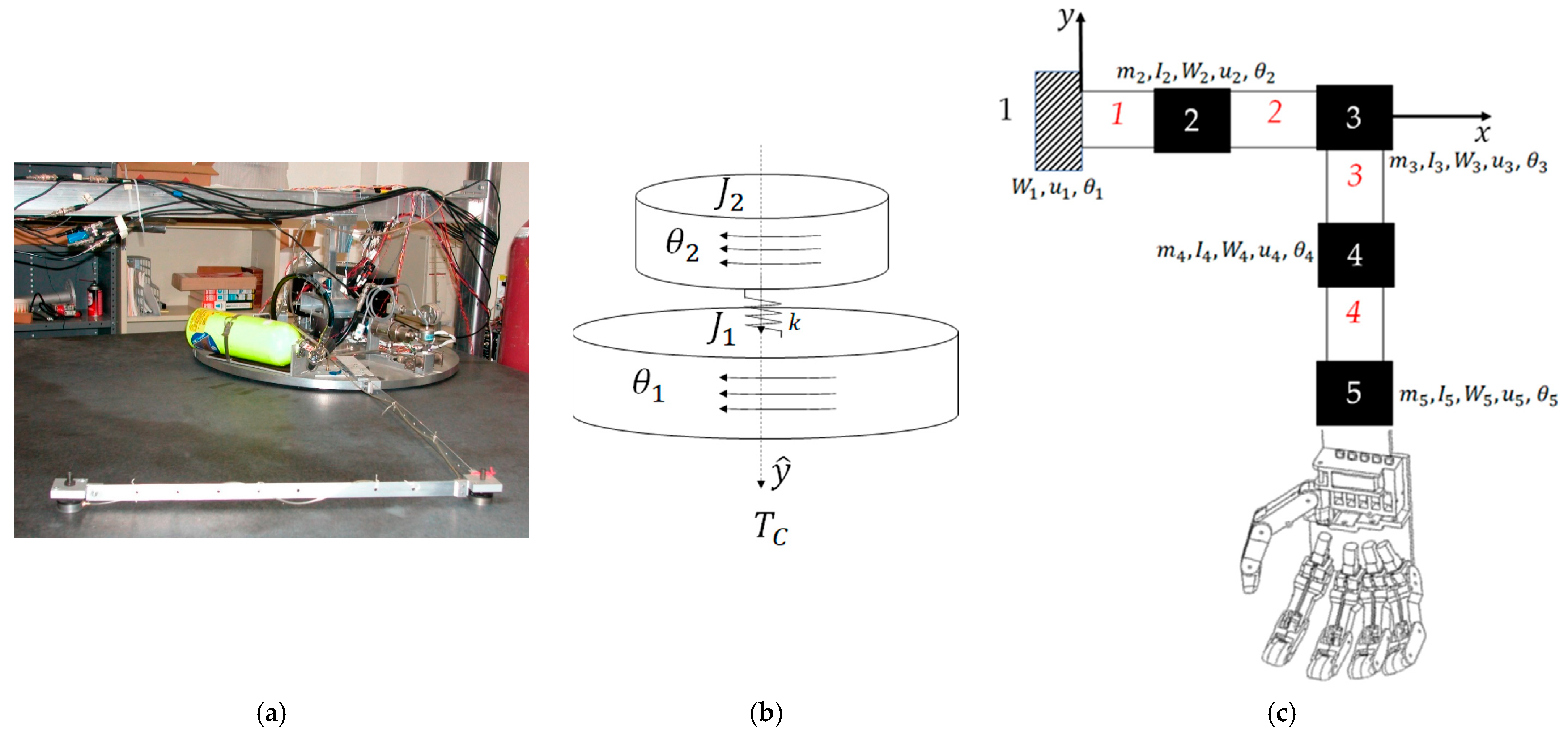
2.1. Space Robot Modeling
| Variable/Acronym | Definition | Variable/Acronym | Definition |
|---|---|---|---|
| Centerline unit vector | Appendage stiffness | ||
| Control torque | Flexible masses and inertias | ||
| Main body inertia mass moment | Flexible inertia mass moment | ||
| Main body rotation angle | Translation and rotation angles |
| Variable/Acronym | Definition |
|---|---|
| , | Externally applied force and torque expressed in inertial coordinates |
| , | Externally applied force and torque expressed in non-inertial coordinates |
| , | Body’s mass and mass moment of inertia |
| Resulting accelerations expressed in inertial coordinates | |
| , | Angular velocity and acceleration vectors |
| ; | Translational velocity and acceleration vectors |
| Flexible member stiffnesses | |
| Assembled matrices of masses and stiffnesses |
| Variable/Acronym | Definition |
|---|---|
| Body principal moment of inertia with respect to Z-axis | |
| Angular acceleration of the system rotation angle, | |
| Rigid–elastic coupling term | |
| Acceleration in generalized displacement coordinates | |
| Reaction wheel principal moment of inertia with respect to C, Z axis | |
| Angular acceleration of the reaction wheel rotation angle, | |
| Control torque of the spacecraft reaction wheel | |
| Disturbance torques |
2.2. Competing Control Design Methodologies
- Gain stabilization,
- Classical second-order structural filtering,
- Input shaping,
- Whiplash compensation,
- Rigid-body minimum-fuel input trajectory shaping,
- Single-frequency trajectory shaping,
- Flatten the curve to improve stability,
- Flatten the curve to improve trajectory tracking,
- Deterministic artificial intelligence:
- 9.1
- Self-awareness statements, and
- 9.2
- Adaption or optimal learning.
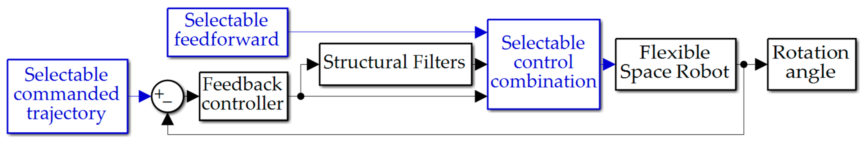
2.3. Selectable Options: Trajectories, Feedforward, Feedback, and Filtering
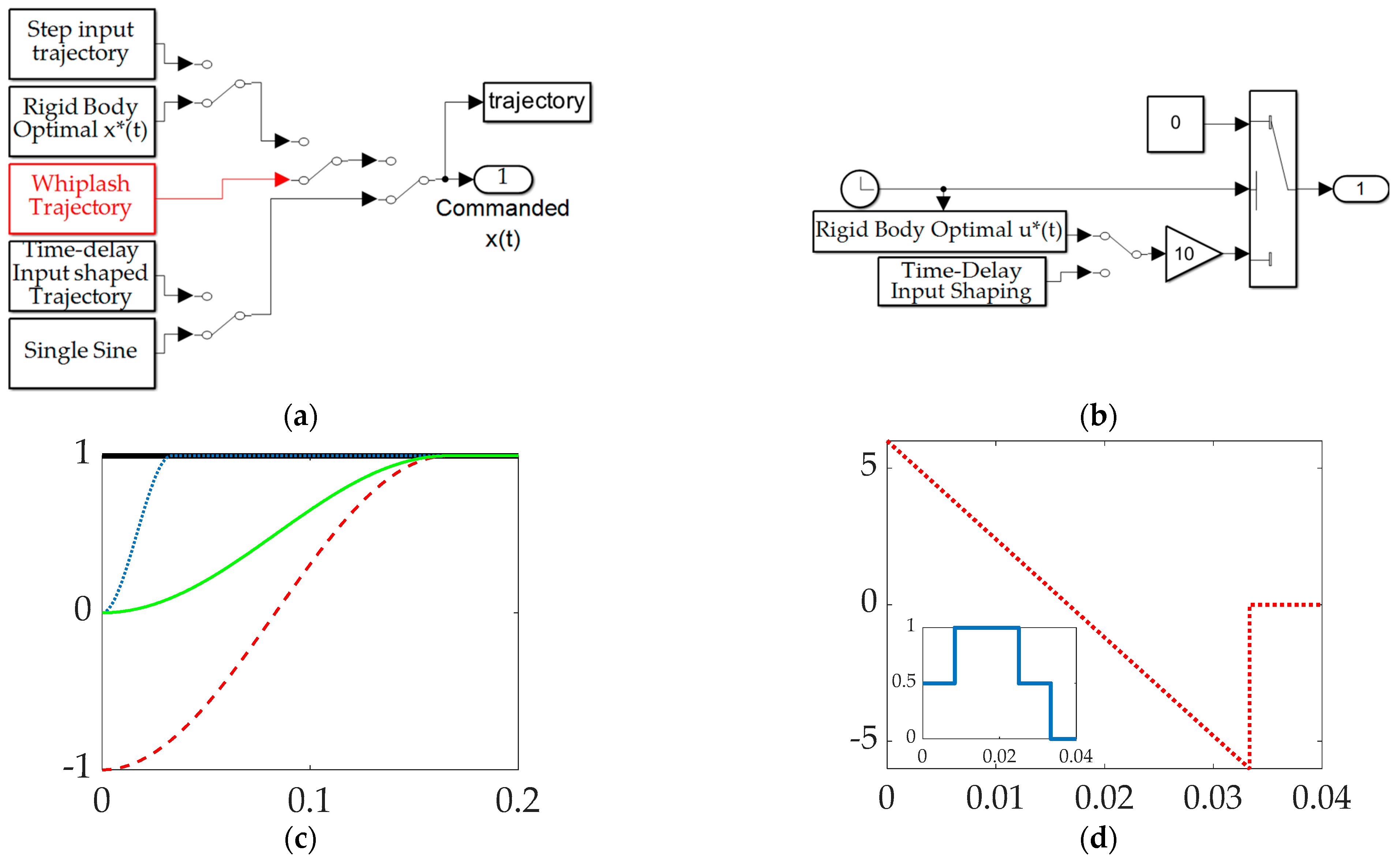
2.3.1. Commanded Trajectories
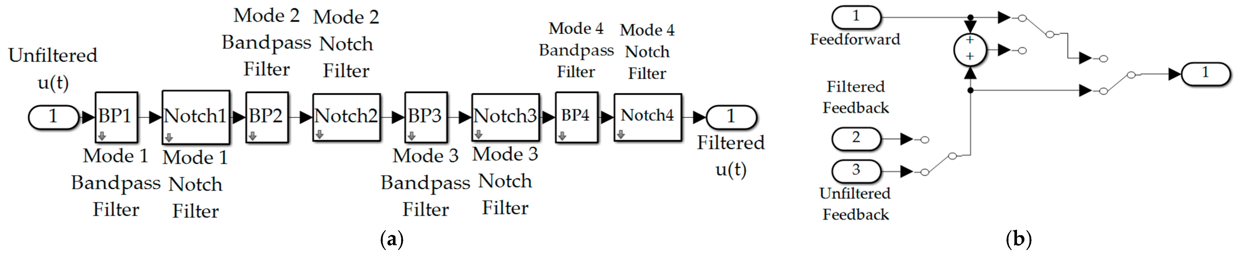
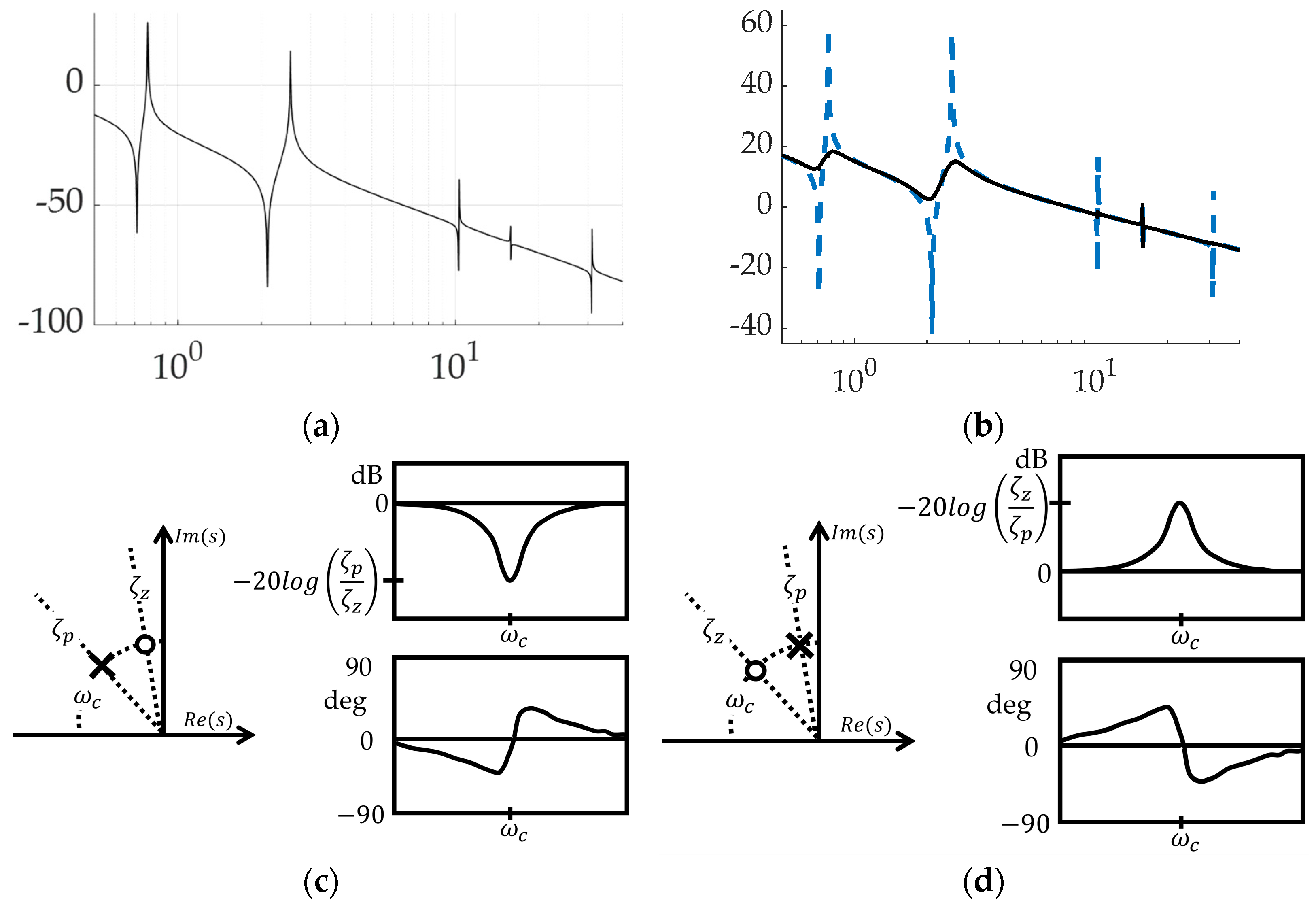
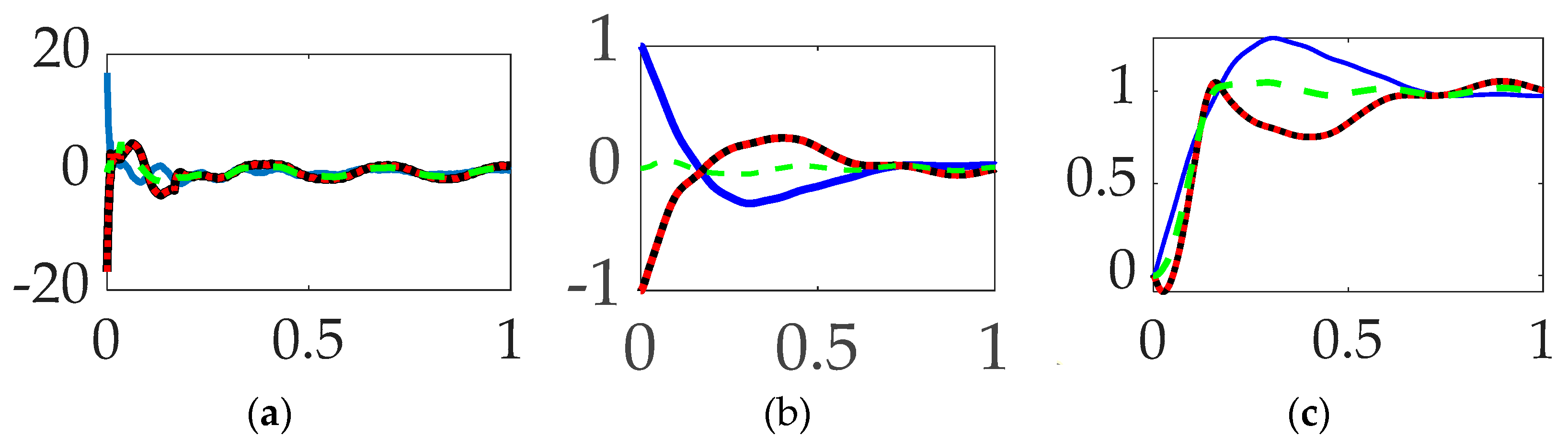
2.3.2. Feedback Filtering


| Variable/ Acronym | Definition |
|---|---|
| Imaginary component of transient response | |
| Real component of transient response | |
| Damping ratio of pole in denominator of Equation (12) | |
| Damping ratio of zero in numerator of Equation (12) | |
| Center frequency of filter placement | |
| Center frequency of filter pole placement in denominator of Equation (12) | |
| Center frequency of filter zero placement in numerator of Equation (12) | |
| dB | Decibels |
| Base-10 logarithm | |
| Displacement or rotation expressed in Laplace domain | |
| Control force or torque expressed in Laplace domain | |
| Steady state gain | |
| Maximum phase lead occurring at frequencies determined by and | |
| Maximum gain occurring when |
2.3.3. Feedforward Controls
3. Results
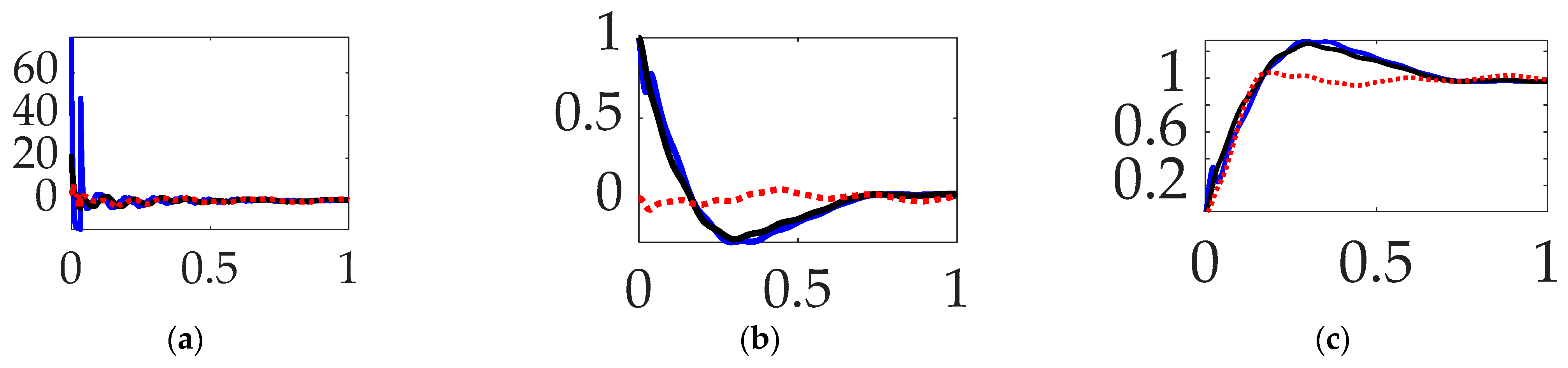
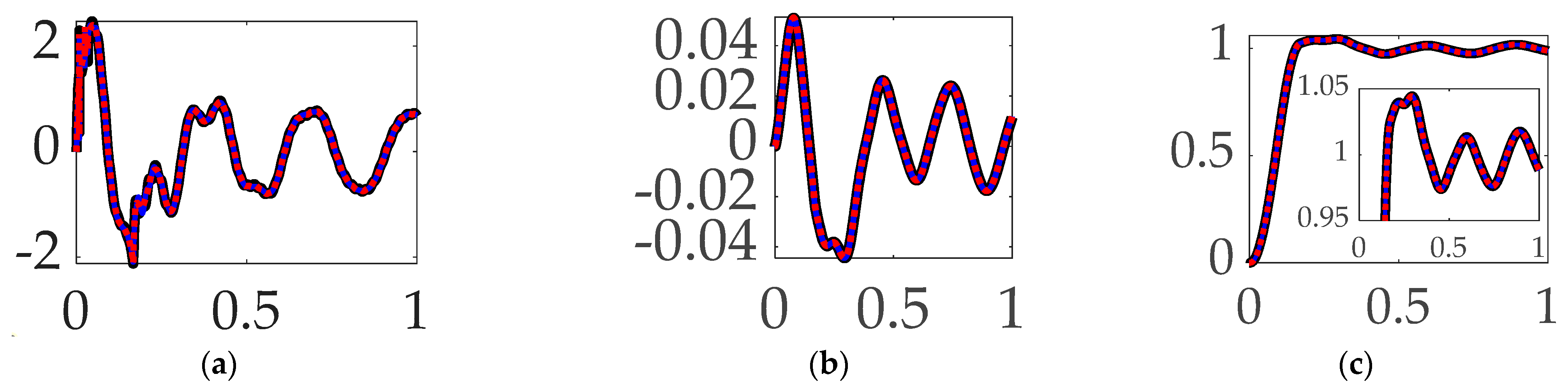
3.1. Comparing Commanded Trajectories with Unfiltered Feedback
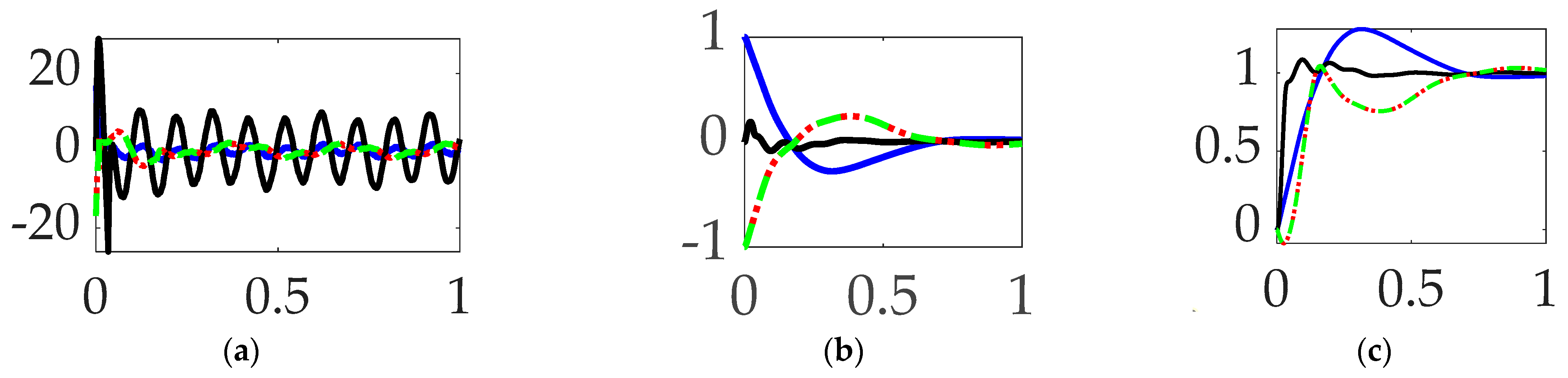
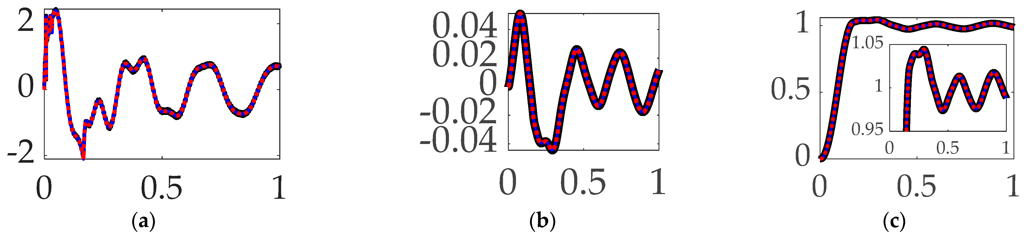
3.2. Comparing Feedforward Controls with Unfiltered Feedback
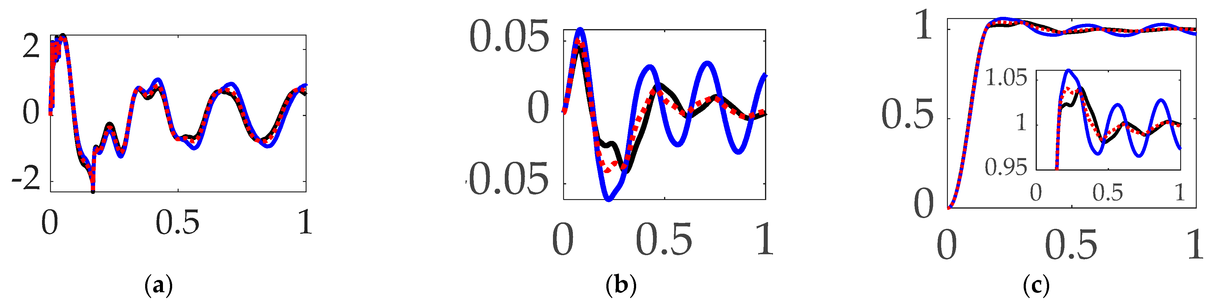
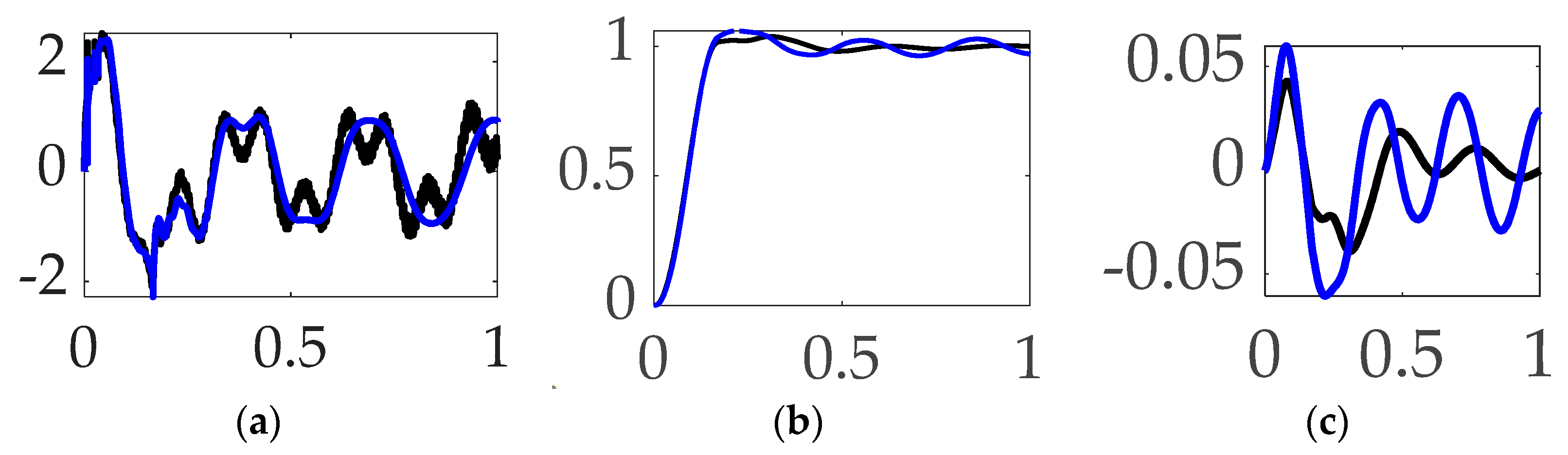
3.3. Comparing Commanded Trajectories with Filtered Feedback
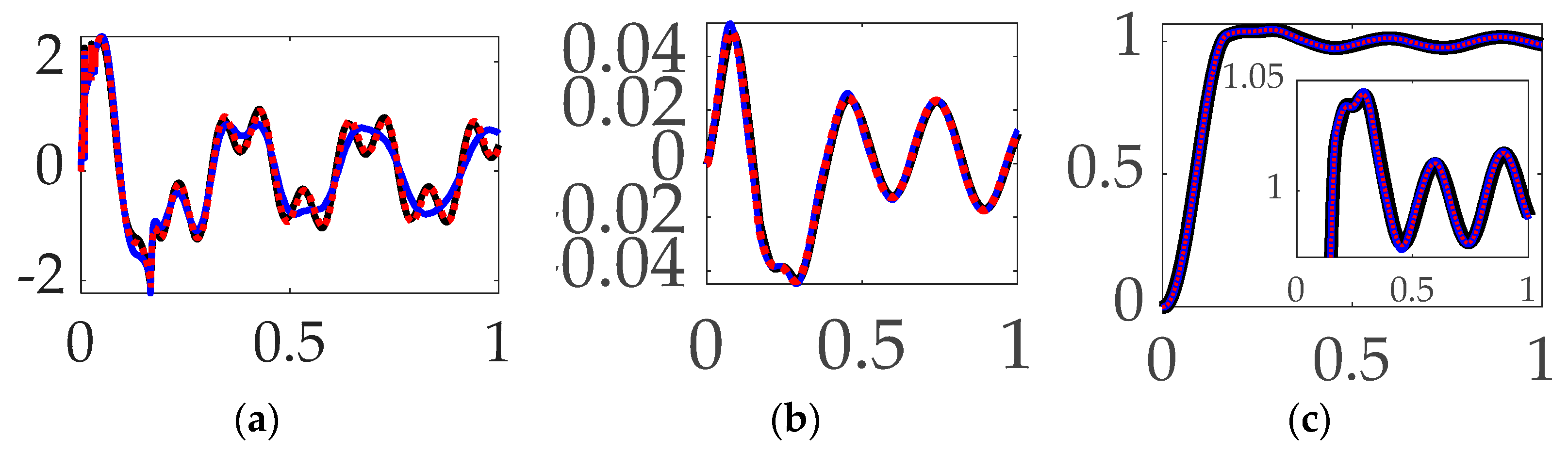
3.4. Comparing Mode 1 Filtering with Single-Sinusoidal Trajectories and No Feedforward
3.5. Comparing Mode 2 Filtering with Single-Sinusoidal Trajectories and No Feedforward
3.6. Comparing Mode 3 Filtering with Single-Sinusoidal Trajectories and No Feedforward
3.7. Comparing Mode 4 Filtering with Single-Sinusoidal Trajectories and No Feedforward
3.8. Comparing Modes 1–4 Filtering with Single-Sinusoidal Trajectories and No Feedforward
3.9. Comparison of the Best Options Studies
4. Discussion
- Bio-inspired trajectory shaping (modified from a time-minimization control per [43]) seems confounded in the presence of classical, unfiltered feedback. While the technique performed well, it was not the exemplary option when compared to the multitude of other available options examined.
- When comparing commanded trajectories, step trajectories surprisingly led to the least control effort, while single-sinusoid trajectories produce the most accurate tracking, with 150% more control effort. The bio-inspired whiplash shaping was optimized in the cited literature for minimum time in a feedforward control sense, while this sequel reveals that the solution is not minimum effort (fuel), nor minimum time in the presence of feedback.
- When comparing feedforward controls, rigid-body optimal feedforward with step trajectory command surprisingly led to the least control effort, while time-delay input-shaped feedforward with single-sinusoid trajectories commanded produced the most accurate tracking, with 280% more control effort.
- When comparing commanded trajectories with filtered feedback and no feedforward, step trajectory commands surprisingly led to the least control effort, while rigid-body optimal trajectories achieved an order of magnitude higher accuracy with 2345% more control effort.
- When comparing mode 1 filtering options bandpass alone not surprisingly led to the least control effort, but surprisingly also produced the most accurate tracking.
- When comparing mode 3 filtering options bandpass led to the least control effort and also produced the most accurate tracking accuracy.
- When comparing mode 4 filtering options bandpass led to the least control effort and also produced the most accurate tracking accuracy.
- The least control effort was achieved with step trajectories, rigid-body optimal feedforward control and unfiltered feedback, and the effort was 75% less than the average. The best mean tracking error was achieved with sinusoidal trajectories, no feedforward, mode 2 notch filtered, and the tracking error mean was 98% better than the average, while the control effort was 330% higher than the minimum available option. The best tracking error deviation was achieved with sinusoidal trajectories, no feedforward, mode 1–4 bandpass filtered, and the tracking error deviation was 80% better than the average, while the control effort was 42% higher than the minimum available option.
5. Conclusions
5.1. Controversial or Unexpected Results
5.1.1. Best Control Effort
5.1.2. Best Tracking Error Mean
5.1.3. Best Tracking Error Deviation
5.2. Recommended Future Reseach
Deterministic Artificial Intelligence
Funding
Institutional Review Board Statement
Data Availability Statement
Conflicts of Interest
Appendix A. Elaboration of Modal System Identification on the Flexible Robot System
| W2 | θ2 | W3 | θ3 | W4 | θ4 | W5 | θ5 | U6 | θ6 | u7 | θ7 | u8 | θ8 | |
|---|---|---|---|---|---|---|---|---|---|---|---|---|---|---|
| W2 | 958.8179 | 0.0000 | −479.409 | 59.9261 | 0 | 0 | 0 | 0 | 0 | 0 | 0 | 0 | 0 | 0 |
| θ2 | 0.0000 | 19.9754 | −59.9261 | 4.9938 | 0 | 0 | 0 | 0 | 0 | 0 | 0 | 0 | 0 | 0 |
| W3 | −479.409 | −59.926 | 958.8179 | 0.0000 | −479.409 | 59.9261 | 0 | 0 | 0 | 0 | 0 | 0 | 0 | 0 |
| θ3 | 59.9261 | 4.9938 | 0.0000 | 19.9754 | −59.9261 | 4.9938 | 0 | 0 | 0 | 0 | 0 | 0 | 0 | 0 |
| W4 | 0 | 0 | −479.409 | −59.926 | 958.8179 | 0.0000 | −479.409 | 59.9261 | 0 | 0 | 0 | 0 | 0 | 0 |
| θ4 | 0 | 0 | 59.9261 | 4.9938 | 0.0000 | 19.9754 | −59.9261 | 4.9938 | 0 | 0 | 0 | 0 | 0 | 0 |
| W5 | 0 | 0 | 0 | 0 | −479.409 | −59.926 | 479.409 | −59.926 | 0 | 0 | 0 | 0 | 0 | 0 |
| θ5 | 0 | 0 | 0 | 0 | 59.9261 | 4.9938 | −59.9261 | 19.9754 | −59.9261 | 4.9938 | 0 | 0 | 0 | 0 |
| U6 | 0 | 0 | 0 | 0 | 0 | 0 | 0 | −59.926 | 958.8179 | 0.0000 | −479.409 | 59.9261 | 0 | 0 |
| θ6 | 0 | 0 | 0 | 0 | 0 | 0 | 0 | 4.9938 | 0.0000 | 19.9754 | −59.9261 | 4.9938 | 0 | 0 |
| U7 | 0 | 0 | 0 | 0 | 0 | 0 | 0 | 0 | −479.409 | −59.926 | 958.8179 | 0.0000 | −479.409 | 59.9261 |
| θ7 | 0 | 0 | 0 | 0 | 0 | 0 | 0 | 0 | 59.9261 | 4.9938 | 0.0000 | 19.9754 | −59.9261 | 4.9938 |
| U8 | 0 | 0 | 0 | 0 | 0 | 0 | 0 | 0 | 0 | 0 | −479.409 | −59.926 | 479.4089 | −59.926 |
| θ8 | 0 | 0 | 0 | 0 | 0 | 0 | 0 | 0 | 0 | 0 | 59.9261 | 4.9938 | −59.9261 | 9.9877 |
| Mass | W2 | θ2 | W3 | θ3 | W4 | θ4 | W5 | θ5 | U6 | θ6 | u7 | θ7 | u8 | θ8 |
|---|---|---|---|---|---|---|---|---|---|---|---|---|---|---|
| W2 | 0.4761 | 0.0000 | 0.0037 | −0.0002 | 0 | 0 | 0 | 0 | 0 | 0 | 0 | 0 | 0 | 0 |
| θ2 | 0.0000 | 0.0000 | 0.0002 | −0.0001 | 0 | 0 | 0 | 0 | 0 | 0 | 0 | 0 | 0 | 0 |
| W3 | 0.0037 | 0.0002 | 4.76 × 10⁻¹ | 0.0000 | 0.0037 | −0.0002 | 0 | 0 | 0 | 0 | 0 | 0 | 0 | 0 |
| θ3 | −0.0002 | −0.0001 | 0.0000 | 0.0000 | 0.0002 | −0.0001 | 0 | 0 | 0 | 0 | 0 | 0 | 0 | 0 |
| W4 | 0 | 0 | 0.0037 | 0.0002 | 0.4761 | 0.0000 | 0.0037 | −0.0002 | 0 | 0 | 0 | 0 | 0 | 0 |
| θ4 | 0 | 0 | −0.0002 | −0.0001 | 0.0000 | 0.0000 | 0.0002 | −0.0001 | 0 | 0 | 0 | 0 | 0 | 0 |
| W5 | 0 | 0 | 0 | 0 | 0.0037 | 0.0002 | 2.63 × 100 | −0.0004 | 0 | 0 | 0 | 0 | 0 | 0 |
| θ5 | 0 | 0 | 0 | 0 | −0.0002 | −0.0001 | −0.0004 | 0.0000 | 0.0002 | −0.0001 | 0 | 0 | 0 | 0 |
| U6 | 0 | 0 | 0 | 0 | 0 | 0 | 0 | 0.0002 | 4.76 × 10⁻¹ | 0.0000 | 0.0037 | −0.0002 | 0 | 0 |
| θ6 | 0 | 0 | 0 | 0 | 0 | 0 | 0 | −0.0001 | 0.00 × 100 | 0.0000 | 0.0002 | −0.0001 | 0 | 0 |
| U7 | 0 | 0 | 0 | 0 | 0 | 0 | 0 | 0 | 0.0037 | 0.0002 | 0.4761 | 0.0000 | 0.0037 | −0.0002 |
| θ7 | 0 | 0 | 0 | 0 | 0 | 0 | 0 | 0 | −0.0002 | −0.0001 | 0.0000 | 0.0000 | 0.0002 | −0.0001 |
| U8 | 0 | 0 | 0 | 0 | 0 | 0 | 0 | 0 | 0 | 0 | 0.0037 | 0.0002 | 4.66 × 10⁻¹ | −0.0004 |
| θ8 | 0 | 0 | 0 | 0 | 0 | 0 | 0 | 0 | 0 | 0 | −0.0002 | −0.0001 | −0.0004 | 0.0000 |
| 1809.5 | 1415.5 | 1042.2 | 774.3 | 596.8 |
| 478.8 | 410.9 | 54.9 | 43.7 | 30.9 |
| 15.8 | 10.2 | 0.7 | 2.1 |
| −1 | 3 | 2 | 0 | −3 | −5 | 3 | 1501 | 383 | 1037 | 443 | −692 | 181 | 240 |
| −1097 | 3080 | 4481 | 4992 | 4505 | 3173 | −1154 | −4544 | −136 | 2388 | 2221 | 4049 | 1395 | 1669 |
| −1 | 1 | −3 | −7 | −5 | 1 | −2 | −1569 | −215 | 204 | 667 | 1425 | −670 | −712 |
| −2158 | 4857 | 3958 | 28 | −3814 | −4883 | 2208 | −943 | −2040 | −7064 | −867 | 912 | −2460 | −1864 |
| −1 | −1 | −5 | 0 | 7 | 3 | 2 | 1296 | −125 | −1076 | 125 | 995 | −1385 | −1057 |
| −3111 | 4495 | −1058 | −4992 | −1185 | 4481 | −3142 | 5806 | 2118 | 368 | −2572 | 4061 | −3204 | −683 |
| 0 | 0 | 0 | 1 | 1 | −1 | 1 | −99 | 30 | 113 | −105 | 248 | 2247 | 954 |
| −3902 | 2199 | −4861 | −47 | 4875 | −2071 | 3937 | −4288 | −3426 | 4504 | 1878 | 4753 | −3652 | 1689 |
| 0 | −3 | 4 | 0 | −6 | 6 | 1 | 536 | −918 | 135 | 898 | 754 | −946 | 736 |
| −4493 | −1062 | −3138 | 4985 | −3062 | −1232 | −4519 | 815 | 2292 | −2423 | 3091 | 891 | −3893 | 3998 |
| 0 | 2 | 5 | −7 | 7 | −4 | 0 | −294 | 753 | 446 | 880 | 410 | −1936 | 1905 |
| −4872 | −3903 | 2129 | 75 | −2232 | 3920 | 4832 | −2471 | 3385 | −210 | −3658 | 3392 | −4013 | 5178 |
| −1 | −2 | 2 | −3 | 4 | −5 | −6 | 90 | −261 | 192 | −699 | −732 | −2945 | 3254 |
| −5031 | −5052 | 5012 | −5030 | 5062 | −4984 | −4965 | 3580 | −7823 | 3941 | −7649 | −5153 | −4046 | 5502 |

Equations of Motion in the Standard State Space Form
| 1 | 2 | 3 | 4 | 5 | 6 | 7 | 8 | 9 | 10 | 11 | 12 | |
|---|---|---|---|---|---|---|---|---|---|---|---|---|
| 1 | 0 | 0 | 0 | 0 | 0 | 0 | 1 | 0 | 0 | 0 | 0 | 0 |
| 2 | 0 | 0 | 0 | 0 | 0 | 0 | 0 | 1 | 0 | 0 | 0 | 0 |
| 3 | 0 | 0 | 0 | 0 | 0 | 0 | 0 | 0 | 1 | 0 | 0 | 0 |
| 4 | 0 | 0 | 0 | 0 | 0 | 0 | 0 | 0 | 0 | 1 | 0 | 0 |
| 5 | 0 | 0 | 0 | 0 | 0 | 0 | 0 | 0 | 0 | 0 | 1 | 0 |
| 6 | 0 | 0 | 0 | 0 | 0 | 0 | 0 | 0 | 0 | 0 | 0 | 1 |
| 7 | 0 | 0.099 | −1.064 | −3.382 | −0.736 | −26.635 | 0 | 1.392 × 10⁻⁴ | −5.066 × 10⁻⁴ | −3.298 × 10⁻⁴ | −4.662 × 10⁻⁵ | −8.609 × 10⁻⁴ |
| 8 | 0 | −0.659 | 1.642 | 5.218 | 1.136 | 41.100 | 0 | −9.264 × 10⁻⁴ | 7.817 × 10⁻⁴ | 5.088 × 10⁻⁴ | 7.194 × 10⁻⁵ | 1.328 × 10⁻³ |
| 9 | 0 | 0.188 | −6.435 | −6.433 | −1.401 | −50.670 | 0 | 2.649 × 10⁻⁴ | −3.064 × 10⁻³ | −6.273 × 10⁻⁴ | −8.869 × 10⁻⁵ | −1.638 × 10⁻³ |
| 10 | 0 | 0.025 | −0.270 | −106.024 | −0.187 | −6.755 | 0 | 3.531 × 10⁻⁵ | −1.285 × 10⁻⁴ | −1.034 × 10⁻² | −1.182 × 10⁻⁵ | −2.183 × 10⁻⁴ |
| 11 | 0 | 0.002 | −0.025 | −0.079 | −249.447 | −0.620 | 0 | 3.241 × 10⁻⁶ | −1.179 × 10⁻⁵ | −7.677 × 10⁻⁶ | −1.579 × 10⁻² | −2.004 × 10⁻⁵ |
| 12 | 0 | 0.022 | −0.233 | −0.742 | −0.162 | −962.998 | 0 | 3.055 × 10⁻⁵ | −1.112 × 10⁻⁴ | −7.237 × 10⁻⁵ | −1.023 × 10⁻⁵ | −3.113 × 10⁻² |
Appendix B. Initialization Function Callbacks for Simulation
| clear all; close all; clc; %This block of code establishes the properties of each beam element a=0.0254; b=0.0016; L=0.25; E=72*10^9; I=a*b^3/12; Li=[12 6*L -12 6*L;6*L 4*L^2 -6*L 2*L^2;-12 -6*L 12 -6*L;6*L 2*L^2 -6*L 4*L^2]; k_beam=E*I/L^3*[Li]; rho_beam=2.8*10^3; %Beam density kg/m^3 A_beam=a*b; %Beam cross sectional area mb=rho_beam*A_beam; %Beam mass per unit length %This block creates the empty stiffness matrix [k] k=zeros(14,14); % This block fills in the stiffness matrix components % Row 1 components start at index=1 % Row 2 components start at index=15 k(1,1)=k_beam(3,3)+k_beam(1,1); k(2,1)=k_beam(4,3)+k_beam(2,1); k(1,2)=k_beam(3,4)+k_beam(1,2); k(2,2)=k_beam(4,4)+k_beam(2,2); k(1,3)=k_beam(1,3); k(2,3)=k_beam(2,3); k(1,4)=k_beam(1,4); k(2,4)=k_beam(2,4); % Row 3 components start at index=29 % Row 4 components start at index=43 k(3,1)=k_beam(3,1); k(4,1)=k_beam(4,1); k(3,2)=k_beam(3,2); k(4,2)=k_beam(4,2); k(3,3)=k_beam(3,3)+k_beam(1,1); k(4,3)=k_beam(4,3)+k_beam(2,1); k(3,4)=k_beam(3,4)+k_beam(1,2); k(4,4)=k_beam(4,4)+k_beam(2,2); k(3,5)=k_beam(1,3); k(4,5)=k_beam(2,3); k(3,6)=k_beam(1,4); k(4,6)=k_beam(2,4); % Row 5 components start at index=59 % Row 6 components start at index=73 k(5,3)=k_beam(3,1); k(6,3)=k_beam(4,1); k(5,4)=k_beam(3,2); k(6,4)=k_beam(4,2); k(5,5)=k_beam(3,3)+k_beam(1,1); k(6,5)=k_beam(4,3)+k_beam(2,1); k(5,6)=k_beam(3,4)+k_beam(1,2); k(6,6)=k_beam(4,4)+k_beam(2,2); k(5,7)=k_beam(1,3); k(6,7)=k_beam(2,3); k(5,8)=k_beam(1,4); k(6,8)=k_beam(2,4); % Row 7 components start at index=89 % Row 8 components start at index=103 k(7,5)=k_beam(3,1); k(8,5)=k_beam(4,1); k(7,6)=k_beam(3,2); k(8,6)=k_beam(4,2); k(7,7)=k_beam(3,3); k(8,7)=k_beam(4,3); k(7,8)=k_beam(3,4); k(8,8)=k_beam(4,4)+k_beam(2,2); k(8,9)=k_beam(2,3); k(8,10)=k_beam(2,4); % Row 9 components start at index=120 % Row 10 components start at index=134 k(9,8)=k_beam(3,2); k(10,8)=k_beam(4,2); k(9,9)=k_beam(3,3)+k_beam(1,1); k(10,9)=k_beam(4,3)+k_beam(2,1); k(9,10)=k_beam(3,4)+k_beam(1,2); k(10,10)=k_beam(4,4)+k_beam(2,2); k(9,11)=k_beam(1,3); k(10,11)=k_beam(2,3); k(9,12)=k_beam(1,4); k(10,12)=k_beam(2,4); % Row 11 components start at index=149 % Row 12 components start at index=163 k(11,9)=k_beam(3,1); k(12,9)=k_beam(4,1); k(11,10)=k_beam(3,2); k(12,10)=k_beam(4,2); k(11,11)=k_beam(3,3)+k_beam(1,1); k(12,11)=k_beam(4,3)+k_beam(2,1); k(11,12)=k_beam(3,4)+k_beam(1,2); k(12,12)=k_beam(4,4)+k_beam(2,2); k(11,13)=k_beam(1,3); k(12,13)=k_beam(2,3); k(11,14)=k_beam(1,4); k(12,14)=k_beam(2,4); % Row 13 components start at index=179 % Row 14 components start at index=193 k(13,11)=k_beam(3,1); k(14,11)=k_beam(4,1); k(13,12)=k_beam(3,2); k(14,12)=k_beam(4,2); k(13,13)=k_beam(3,3); k(14,13)=k_beam(4,3); k(13,14)=k_beam(3,4); k(14,14)=k_beam(4,4); %Display stiffness matrix to check k=k; %END STIFFNESS MATRIX. START MASS MATRIX %Assemble individual beam inertia matrix I_beam=ones(1,8); %Creates empty matrix of I’s for eight node points I_beam=[I_beam.*I]; %Fill in matrix values with beam inertia I_beam(1)=0; %First node point inertia = 0 %This block of code creates the individual beam mass matrix “m_beam” mi=[156 22*L 54 -13*L;22*L 4*L^2 13*L -3*L^2;54 13*L 156 -22*L;-13*L -3*L^2 -22*L 4*L^2]; m_beam=mb*L/420*mi; %This block of code establishes the value of each point mass (mp) %and the system point mass matrix (M) mp=0.455; %Point masses, M M=[0 mp mp mp 2*mp mp mp mp]; %Matrix of 8 point masses (0 First point mass) %Creates a 14x14 empty mass matrix [m] m=zeros(14,14); %Fill in the system mass matrix components % Row 1 components start at index=1 % Row 2 components start at index=15 m(1,1)=m_beam(3,3)+m_beam(1,1)+M(2); m(2,1)=m_beam(4,3)+m_beam(2,1); m(1,2)=m_beam(3,4)+m_beam(1,2); m(2,2)=m_beam(4,4)+m_beam(2,2); m(1,3)=m_beam(1,3); m(2,3)=m_beam(2,3); m(1,4)=m_beam(1,4); m(2,4)=m_beam(2,4); % Row 3 components start at index=29 % Row 4 components start at index=43 m(3,1)=m_beam(3,1); m(4,1)=m_beam(4,1); m(3,2)=m_beam(3,2); m(4,2)=m_beam(4,2); m(3,3)=m_beam(3,3)+m_beam(1,1)+M(3); m(4,3)=m_beam(4,3)+m_beam(2,1); m(3,4)=m_beam(3,4)+m_beam(1,2); m(4,4)=m_beam(4,4)+m_beam(2,2); m(3,5)=m_beam(1,3); m(4,5)=m_beam(2,3); m(3,6)=m_beam(1,4); m(4,6)=m_beam(2,4); % Row 5 components start at index=59 % Row 6 components start at index=73 m(5,3)=m_beam(3,1); m(6,3)=m_beam(4,1); m(5,4)=m_beam(3,2); m(6,4)=m_beam(4,2); m(5,5)=m_beam(3,3)+m_beam(1,1)+M(4); m(6,5)=m_beam(4,3)+m_beam(2,1); m(5,6)=m_beam(3,4)+m_beam(1,2); m(6,6)=m_beam(4,4)+m_beam(2,2); m(5,7)=m_beam(1,3); m(6,7)=m_beam(2,3); m(5,8)=m_beam(1,4); m(6,8)=m_beam(2,4); % Row 7 components start at index=89 m(7,5)=m_beam(3,1); m(7,6)=m_beam(3,2); m(7,7)=m_beam(3,3)+3*mb+M(5)+M(6)+M(7)+M(8); m(7,8)=m_beam(3,4); % Row 8 components start at index=103 % Row 9 components start at index=120 m(8,5)=m_beam(4,1); m(9,8)=m_beam(3,2); m(8,6)=m_beam(4,2); m(9,9)=m_beam(3,3)+m_beam(1,1)+M(6); m(8,7)=m_beam(4,3); m(9,10)=m_beam(3,4)+m_beam(1,2); m(8,8)=m_beam(4,4)+m_beam(2,2); m(9,11)=m_beam(1,3); m(8,9)=m_beam(2,3); m(9,12)=m_beam(1,4); m(8,10)=m_beam(2,4); % Row 10 components start at index=134 % Row 11 components start at index=149 m(10,8)=m_beam(4,2); m(11,9)=m_beam(3,1); m(10,9)=m_beam(4,3)+m_beam(2,1); m(11,10)=m_beam(3,2); m(10,10)=m_beam(4,4)+m_beam(2,2); m(11,11)=m_beam(3,3)+m_beam(1,1)+M(7); m(10,11)=m_beam(2,3); m(11,12)=m_beam(3,4)+m_beam(1,2); m(10,12)=m_beam(2,4); m(11,13)=m_beam(1,3); m(11,14)=m_beam(1,4); % Row 12 components start at index=163 m(12,9)=m_beam(4,1); m(12,10)=m_beam(4,2); m(12,11)=m_beam(4,3)+m_beam(2,1); m(12,12)=m_beam(4,4)+m_beam(2,2); m(12,13)=m_beam(2,3); m(12,14)=m_beam(2,4); % Row 13 components start at index=179 % Row 14 components start at index=193 m(13,11)=m_beam(3,1); m(14,11)=m_beam(4,1); m(13,12)=m_beam(3,2); m(14,12)=m_beam(4,2); m(13,13)=m_beam(3,3)+M(8); m(14,13)=m_beam(4,3); m(13,14)=m_beam(3,4); m(14,14)=m_beam(4,4); %Display the system mass matrix to check m=m; %Calculate the natural frequencies and normal modes [NormalModes,EigenValues]=eig(inv(m)*k); NaturalFrequencies=diag(EigenValues^0.5); ModeShapes=NormalModes; %Check Orthogonality like Homework 1 confirm diagonal matrix of 1’s %to satisfy equation 24 on slide 17 OrthoMass=NormalModes’*m*NormalModes; OrthoStiff=NormalModes’*k*NormalModes; StiffCheck=OrthoStiff/EigenValues; Equation24_OrthoCheck=diag(diag(StiffCheck/OrthoMass)); %Spacecraft Radius to be used designating rigid modal coordinate R=0.381; FeeE=NormalModes; %Designate Elastic mode shapes array FeeE Omega=NaturalFrequencies; %Designate variable name ‘Omega’ as natural frequencies %Designate Rigid modal coordinate FeeR FeeR=[R+L 1 R+L*2 1 R+L*3 1 R+L*4 1 -L 1 -L*2 1 -L*3 1]; Di=FeeE’*m*diag(FeeR); %Calculate Rigid-Elastic Coupling Coefficient DiCheck=det(Di); %Confirm Di is singular...det(Di=0) Z=0.0005; Izz=14; w=diag(NaturalFrequencies); %Generate a diagonal matrix of natural frequency Iw=0.0912; Td=0; %Disturbance Torque Tc=0.1; %Control Torque is Iw*qddot_wheel T=Td+Tc; %Total Torque is sum of disturbance and control torques %Start State Space Development NatFreq = diag(EigenValues).^0.5; r = 0.381; %Radius of the wheel (large rigid body) freqs = sqrt(EigenValues); % NatFreq = EigenValues(1:5,1:5); freqs = freqs(1:5,1:5); zeta = 0.0005; %Given damping ratio for all modes Izz = 14; phi_E = NormalModes(1:14,1:5); phi_R = [r+L,1,r+2*L,1,r+3*L,1,r+4*L,1,-L,1,-2*L,1,-3*L,1]’; M_II = m; Di = [phi_E’*M_II*phi_R]; M_state = [Izz Di’; Di eye(5)]; C_damp = [zeros(6,6)]; C_damp(2:6,2:6) = 2*zeta*freqs; K=[zeros(6,6)]; K(2:6,2:6) = NatFreq; A = [zeros(6),eye(6,6); -inv(M_state)*K, -inv(M_state)*C_damp]; Bprime = [1;0;0;0;0;0]; B = [0 0 0 0 0 0 (inv(M_state)*Bprime)’]’; C = zeros(12,12); C(1,1)=1; D = zeros(12,1); [Gnum,Gden] = ss2tf(A,B,C,D); G1 = tf(Gnum(1,:),Gden) %Manually input Transfer Function to check NUM=[1.998e-015 0.1268 0.007582 166.9 5.591 4.718e004 771 3.412e006 1.218e004 1.576e007 1.475e004 7.11e006]; DEN=[1 0.06125 1326 46.15 3.781e005 6683 2.808e007 1.388e005 1.813e008 2.065e005 9.954e007 0 0]; G=tf(NUM,DEN); %Put PID controller Transfer function into workspace It=14; Z=0.516931; Bandwidth=4; wn=Bandwidth; T=10/Z/wn; Kd=2*Z*wn*It+It/T; Kp=wn^2+2*Z*wn/T; Ki=wn^2/T; PID=tf([Kd Kp Ki],[0 1 0]); %DESIGN FILTERS TO SMOOTH OUT MODE 1 %Design Bandpass filter for w = 10^-0.1478 = 0.711541 Hz wz=0.711541;Zz=0.1;wp=wz;Zp=0.0005; BP1=tf([1/wz^2 2*Zz/wz 1],[1/wp^2 2*Zp/wp 1]); PID_BP1=PID*BP1; %Design Notch filter for w = 10^-0.109 = 0.778037 Hz wz=0.778037;Zz=0.0005;wp=wz;Zp=0.1; Notch1=tf([1/wz^2 2*Zz/wz 1],[1/wp^2 2*Zp/wp 1]); Mode_1=PID*BP1*Notch1; %DESIGN FILTERS TO SMOOTH OUT MODE 2 %Design Bandpass filter for w = 10^0.3223 wz=10^0.3223;Zz=0.1;wp=wz;Zp=0.0005; BP2=tf([1/wz^2 2*Zz/wz 1],[1/wp^2 2*Zp/wp 1]); %Design Notch filter for w = 10^0.405 wz=10^0.405;Zz=0.0006;wp=wz;Zp=0.1; Notch2=tf([1/wz^2 2*Zz/wz 1],[1/wp^2 2*Zp/wp 1]); Mode_2=Mode_1*BP2*Notch2; %Design Lead filter for wz~1, wp~3 %wz=1;Zz=1;wp=3;Zp=1; %Lead=tf([1/wz^2 2*Zz/wz 1],[1/wp^2 2*Zp/wp 1]); %Mode_2=Mode_2*Lead; %DESIGN FILTERS TO SMOOTH OUT MODE 3 %Design Bandpass filter for w = 10^1.0110 wz=10^1.0110;Zz=0.1;wp=wz;Zp=0.0005; BP3=tf([1/wz^2 2*Zz/wz 1],[1/wp^2 2*Zp/wp 1]); %Design Notch filter for w = 10^1.0128 wz=10^1.0128;Zz=0.0005;wp=wz;Zp=0.1; Notch3=tf([1/wz^2 2*Zz/wz 1],[1/wp^2 2*Zp/wp 1]); Mode_3=Mode_2*BP3*Notch3; %DESIGN FILTERS TO SMOOTH OUT MODE 4 %Design Bandpass filter for w = 10^1.49035 wz=10^1.49035;Zz=0.1;wp=wz;Zp=0.0005; BP4=tf([1/wz^2 2*Zz/wz 1],[1/wp^2 2*Zp/wp 1]); %Design Notch filter for w = 10^1.492 wz=10^1.492;Zz=0.0005;wp=wz;Zp=0.1; Notch4=tf([1/wz^2 2*Zz/wz 1],[1/wp^2 2*Zp/wp 1]); Mode_4=Mode_3*BP4*Notch4; %CALCULATE SYSTEM NATURAL FREQUENCIES [NaturalFrequencies,Damping,EigenValue]=damp(G); NaturalFrequencies=NaturalFrequencies; |
Appendix C. Stop Function Callbacks for Simulation
| [mag1,phase1,wout1] = bode(G); Mag1=20*log10(mag1(:)); Phase1=phase1(:); [mag2,phase2,wout2] = bode(G*PID); Mag2=20*log10(mag2(:)); Phase2=phase2(:); [mag3,phase3,wout3] = bode(G*PID*BP1); Mag3=20*log10(mag3(:)); Phase3=phase3(:); [mag4,phase4,wout4] = bode(G*PID*BP1*Notch1); Mag4=20*log10(mag4(:)); Phase4=phase4(:); [mag5,phase5,wout5] = bode(G*PID*BP1*Notch1*BP2); Mag5=20*log10(mag5(:)); Phase5=phase5(:); [mag6,phase6,wout6] = bode(G*PID*BP1*Notch1*BP2*Notch2); Mag6=20*log10(mag6(:)); Phase6=phase6(:); [mag7,phase7,wout7] = bode(G*PID*BP1*Notch1*BP2*Notch2*BP3); Mag7=20*log10(mag7(:)); Phase7=phase7(:); [mag8,phase8,wout8] = bode(G*PID*BP1*Notch1*BP2*Notch2*BP3*Notch3); Mag8=20*log10(mag8(:)); Phase8=phase8(:); [mag9,phase9,wout9] = bode(G*PID*BP1*Notch1*BP2*Notch2*BP3*Notch3*BP4); Mag9=20*log10(mag9(:)); Phase9=phase9(:); [mag10,phase10,wout10] = bode(G*PID*BP1*Notch1*BP2*Notch2*BP3*Notch3*BP4*Notch4); Mag10=20*log10(mag10(:)); Phase10=phase10(:); figure(1); hold on; semilogx(wout1,Mag1,‘--’,‘LineWidth’,1); semilogx(wout2,Mag2,‘LineWidth’,1); semilogx(wout3,Mag3,‘--’,‘LineWidth’,3); semilogx(wout4,Mag4,‘:’,‘LineWidth’,2); hold off; grid on; axis([0.5,40, -100, 150 ]); set(gca, ‘FontSize’,28, ‘FontName’,‘Palatino Linotype’); legend(‘Flexible space robot’,‘PID’,‘PID + Bandpass’,‘PID + Notch + Bandpass’) figure(2); hold on; set(gca, ‘FontSize’,28, ‘FontName’,‘Palatino Linotype’); semilogx(wout1,Phase1,’--’,‘LineWidth’,1); semilogx(wout2,Phase2,’LineWidth’,1); semilogx(wout3,Phase3,’--’,‘LineWidth’,3); semilogx(wout4,Phase4,’:’,‘LineWidth’,2); hold off; grid on; figure(3); hold on; semilogx(wout2,Mag2,’--’,‘LineWidth’,1); semilogx(wout4,Mag4,’LineWidth’,1); semilogx(wout5,Mag5,’--’,‘LineWidth’,3); semilogx(wout6,Mag6,’:’,‘LineWidth’,2); hold off; grid on; axis([0.5,40, -100, 150 ]); set(gca, ‘FontSize’,28, ‘FontName’,‘Palatino Linotype’); legend(‘PID controlled Flexible space robot’,‘PID+Mode 1’,‘PID + Mode 1 + Bandpass’,‘PID + Mode 1 + Notch + Bandpass’) figure(4); hold on; set(gca, ‘FontSize’,28, ‘FontName’,‘Palatino Linotype’); semilogx(wout2,Phase2,’--’,‘LineWidth’,1); semilogx(wout4,Phase4,’LineWidth’,1); semilogx(wout5,Phase5,’--’,‘LineWidth’,3); semilogx(wout6,Phase6,’:’,‘LineWidth’,2); hold off; grid on; figure(5); hold on; semilogx(wout2,Mag2,’--’,‘LineWidth’,1); semilogx(wout4,Mag4,’LineWidth’,1); semilogx(wout6,Mag6,’--’,‘LineWidth’,3); semilogx(wout7,Mag7,’:’,‘LineWidth’,2); semilogx(wout8,Mag8,’:’,‘LineWidth’,2); hold off; grid on; axis([0.5,40, -100, 150 ]); set(gca, ‘FontSize’,28, ‘FontName’,‘Palatino Linotype’); legend(‘PID controlled Flexible space robot’,‘PID + Mode 1’,‘PID + Mode 2’,‘PID + Mode 1 + Mode 2 + Bandpass’,‘PID + Mode 1 + Mode 2 + Bandpass + Notch’) figure(6); hold on; set(gca, ‘FontSize’,28, ‘FontName’,‘Palatino Linotype’); semilogx(wout2,Phase2,’--’,‘LineWidth’,1); semilogx(wout4,Phase4,’LineWidth’,1); semilogx(wout6,Phase6,’--’,‘LineWidth’,3); semilogx(wout7,Phase7,’:’,‘LineWidth’,2); semilogx(wout8,Phase8,’:’,‘LineWidth’,2); hold off; grid on; figure(7); hold on; semilogx(wout2,Mag2,’--’,‘LineWidth’,1); semilogx(wout4,Mag4,’LineWidth’,1); semilogx(wout6,Mag6,’--’,‘LineWidth’,3); semilogx(wout8,Mag8,’:’,‘LineWidth’,2); semilogx(wout9,Mag9,’:’,‘LineWidth’,2); semilogx(wout10,Mag10,’:’,‘LineWidth’,2); hold off; grid on; axis([0.5,40, -100, 150 ]); set(gca, ‘FontSize’,28, ‘FontName’,‘Palatino Linotype’); legend(‘PID controlled Flexible space robot’,‘PID + Mode 1’,‘PID + Mode 2’,‘PID + Mode 1 + Mode 2 + Mode 3’,‘PID + Mode 1 + Mode 2 + Mode 3 + Bandpass + Notch’) figure(8); hold on; set(gca, ‘FontSize’,28, ‘FontName’,‘Palatino Linotype’); semilogx(wout2,Phase2,’--’,‘LineWidth’,1); semilogx(wout4,Phase4,’LineWidth’,1); semilogx(wout6,Phase6,’--’,‘LineWidth’,3); semilogx(wout8,Phase8,’:’,‘LineWidth’,2); semilogx(wout9,Phase9,’:’,‘LineWidth’,2); semilogx(wout10,Phase10,’:’,‘LineWidth’,2); hold off; grid on; sys1=G*PID/(1+G*PID); sys2=(G*PID*BP1/(1+G*PID*BP1)); sys3=(G*PID*BP1*Notch1/(1+G*PID*BP1*Notch1)); sys4=(G*PID*BP1*Notch1*BP2/(1+G*PID*BP1*Notch1*BP2)); sys5=(G*PID*BP1*Notch1*BP2*Notch2/(1+G*PID*BP1*Notch1*BP2*Notch2)); sys6=(G*PID*BP1*Notch1*BP2*Notch2*BP3/(1+G*PID*BP1*Notch1*BP2*Notch2*BP3)); sys7=(G*PID*BP1*Notch1*BP2*Notch2*BP3*Notch3/(1+G*PID*BP1*Notch1*BP2*Notch2*BP3*Notch3)); sys8=(G*PID*BP1*Notch1*BP2*Notch2*BP3*Notch3*BP4/(1+G*PID*BP1*Notch1*BP2*Notch2*BP3*Notch3*BP4)); sys9=(G*PID*BP1*Notch1*BP2*Notch2*BP3*Notch3*BP4*Notch4/(1+G*PID*BP1*Notch1*BP2*Notch2*BP3*Notch3*BP4*Notch4)); figure(9); step(sys1,sys2); legend(‘PID’,‘PID + BP1’);set(gca, ‘FontSize’,28, ‘FontName’,‘Palatino Linotype’); figure(10); step(sys1,sys3); legend(‘PID’,‘PID + BP1+Notch1’); set(gca, ‘FontSize’,28, ‘FontName’,‘Palatino Linotype’); figure(11); step(sys1,sys4); legend(‘PID’,‘PID + Mode 1 + BP2’); set(gca, ‘FontSize’,28, ‘FontName’,‘Palatino Linotype’); figure(12); step(sys1,sys5); legend(‘PID’,‘PID + Mode 1 + BP2 + Notch 2’); set(gca, ‘FontSize’,28, ‘FontName’,‘Palatino Linotype’); figure(13); step(sys1,sys6); legend(‘PID’,‘PID + Mode 1 + Mode 2 + BP3’); set(gca, ‘FontSize’,28, ‘FontName’,‘Palatino Linotype’); figure(14); step(sys1,sys7); legend(‘PID’,‘PID + Mode 1 + Mode 2 + BP3 + Notch3’); set(gca, ‘FontSize’,28, ‘FontName’,‘Palatino Linotype’); figure(15); step(sys1,sys8); legend(‘PID’,‘PID + Mode 1 + Mode 2 + Mode 3 + BP4’); set(gca, ‘FontSize’,28, ‘FontName’,‘Palatino Linotype’); figure(16); step(sys1,sys9); legend(‘PID’,‘PID + Mode 1 + Mode 2 + Mode 3 + BP4 + Notch4’); set(gca, ‘FontSize’,28, ‘FontName’,‘Palatino Linotype’); |
References
- AF, Navy Baseball Teams Square off for 2018 Freedom Classic. Available online: https://www.nellis.af.mil/News/Article/1452330/af-navy-baseball-teams-square-off-for-2018-freedom-classic/ (accessed on 12 December 2023).
- Department of Defense Policy. U.S. Department of Defense Photographs and Imagery, Unless Otherwise Noted, Are in the Public Domain. Available online: https://www.defense.gov/Contact/Help-Center/Article/article/2762906/use-of-department-of-defense-imagery (accessed on 12 December 2023).
- Nile, R. First Humanoid Robot in Space Receives NASA Government Invention of the Year. 17 June 2015. Available online: https://www.nasa.gov/mission_pages/station/research/news/invention_of_the_year (accessed on 17 February 2023).
- NASA Image Use Policy. NASA Content (Images, Videos, Audio, etc.) Are Generally Not Copyrighted and May Be Used for Educational or Informational Purposes without Needing Explicit Permissions. Available online: https://gpm.nasa.gov/image-use-policy (accessed on 8 October 2023).
- Nesnas, I.; Fesq, L.; Volpe, R. Autonomy for Space Robots: Past, Present, and Future. Curr. Robot. Rep. 2021, 2, 251–263. [Google Scholar] [CrossRef]
- Sagan, C.; Reddy, R. Machine Intelligence and Robotics: Report of the NASA Study Group Final Report. 715-32. Carnegie Mellon University. 1980. Available online: http://www.rr.cs.cmu.edu/NASA%20Sagan%20Report.pdf (accessed on 7 September 2011).
- NASA Autonomous Systems—Systems Capability Leadership Team. Autonomous Systems Taxonomy. NASA Technical Reports Server. 14 May 2018; p. 20180003082. Available online: https://ntrs.nasa.gov/citations/20180003082 (accessed on 8 February 2024).
- Marshall Spaceflight Center, Advanced Space Transportation Program: Paving the Highway to Space. Available online: https://www.nasa.gov/centers/marshall/news/background/facts/astp.html (accessed on 15 January 2022).
- Curiosity Bot, Advantages and Disadvantages of Using Robots Instead of Astronauts. Available online: https://mycuriositybot.wordpress.com/2019/02/18/advantages–and–disadvantages–of–using–robots–instead–of–astronauts/ (accessed on 18 February 2019).
- NASA Is Building a Mission That Will Refuel and Repair Satellites in Orbit. Available online: https://www.universetoday.com/155863/nasa-is-building-a-mission-that-will-refuel-and-repair-satellites-in-orbit/ (accessed on 8 October 2023).
- DARPA Teams with Northrop Grumman to Build Robotic Service Satellites. Available online: https://newatlas.com/space/robotic-service-satellite-darpa-northrop-grumman/ (accessed on 8 October 2023).
- Usage Policy. Images Posted on the DARPA Website May Be Used for Educational or Informational Purposes. Available online: https://www.darpa.mil/policy/usage-policy (accessed on 8 October 2023).
- Holzinger, M.; Chow, C.; Garretson, P. A Primer on Cislunar Space; Technical Report; Air Force Research Labs: Wright-Patterson Air Force Base, OH, USA, 7 May 2021; Available online: https://www.afrl.af.mil/Portals/90/Documents/RV/A%20Primer%20on%20Cislunar%20Space_Dist%20A_PA2021-1271.pdf?ver=vs6e0sE4PuJ51QC-15DEfg%3d%3d (accessed on 9 October 2023).
- Available online: https://www.ssc.spaceforce.mil/Portals/3/SDA%20Briefings/13.%20Bates_Tyler_SDA%20Industry%20Day_Cislunar%20Space%20SDA_V4.pdf?ver=fhTzhW7RFhI1MDcP90KAuQ%3D%3D (accessed on 14 December 2023).
- Image Created by NASA. Available online: https://en.wikipedia.org/wiki/Halo_orbit#/media/File:Lagrange_points2.svg (accessed on 31 December 2023).
- Ellery, A. Tutorial Review on Space Manipulators for Space Debris Mitigation. Robotics 2019, 8, 34. [Google Scholar] [CrossRef]
- Zhang, W.; Li, F.; Li, J.; Cheng, Q. Review of On-Orbit Robotic Arm Active Debris Capture Removal Methods. Aerospace 2023, 10, 13. [Google Scholar] [CrossRef]
- Jiang, D.; Cai, Z.; Peng, H.; Wu, Z. Coordinated Control Based on Reinforcement Learning for Dual-Arm Continuum Manipulators in Space Capture Missions. J. Aero. Eng. 2021, 34, 04021087. [Google Scholar] [CrossRef]
- Yang, J.; Peng, H.; Zhang, J.; Wu, Z. Dynamic modeling and beating phenomenon analysis of space robots with continuum manipulators. Chin. J. Aero. 2022, 35, 226–241. [Google Scholar] [CrossRef]
- Jiang, D.; Cai, Z.; Liu, Z.; Peng, H. An Integrated Tracking Control Approach Based on Reinforcement Learning for a Continuum Robot in Space Capture Missions. J. Aero. Eng. 2022, 35, 04022065-1. [Google Scholar] [CrossRef]
- Yang, J.; Peng, H.; Zhou, W.; Wu, Z. Integrated Control of Continuum-Manipulator Space Robots with Actuator Saturation and Disturbances. J. Guid. Con. Dyn. 2022, 45, 2379. [Google Scholar] [CrossRef]
- Ai, H.; Zhu, A.; Wang, J.; Yu, X.; Chen, L. Buffer Compliance Control of Space Robots Capturing a Non-Cooperative Spacecraft Based on Reinforcement Learning. Appl. Sci. 2021, 11, 5783. [Google Scholar] [CrossRef]
- Armanini, C.; Boyer, F.; Mathew, A.; Duriez, C.; Renda, F. Soft robots modeling: A structured overview. IEEE Trans. Robot. 2022, 39, 1–21. [Google Scholar] [CrossRef]
- Encyclopaedia Britannica, Britannica, Euclidean Space. Available online: https://www.britannica.com/science/Euclidean–space (accessed on 10 October 2022).
- Newton, I. Principia, Jussu Societatis Regiæ ac Typis Joseph Streater; Cambridge University Library: London, UK, 1687. [Google Scholar]
- Mazalov, V.; Parilina, E. The Euler–equation approach in average–oriented opinion dynamics. Mathematics 2020, 8, 355. [Google Scholar] [CrossRef]
- Sands, T. Comparison and Interpretation Methods for Predictive Control of Mechanics. Algorithms 2019, 12, 232. [Google Scholar] [CrossRef]
- A.C.M. Operations, What–Are–the–6–Degrees–of–Freedom, Industrial Inspection & Analysis (IIA). Available online: https://industrial–ia.com/what–are–the–6–degrees–of–freedom–6dof–explained/ (accessed on 21 March 2023).
- Doyle, J.; Francis, A.; Tannenbaum, A. Feedback Control Theory; Dover: Mineola, NY, USA, 2009. [Google Scholar]
- Johansson, R.; Robertsson, A.; Nilsson, K.; Verhaegen, M. State–Space System Identification of Robot Manipulator Dynamics. Mechatronics 2000, 10, 403–418. [Google Scholar] [CrossRef]
- Corke, P. High–Performance Visual Closed–Loop Robot Control. Ph.D. Thesis, Mechanical and Manufacturing Engineering, University of Melbourne, Melbourne, Australia, 1994. [Google Scholar]
- Li, Y.; Ang, K.; Chong, G.C.Y. PID Control System Analysis and design. IEEE Control Syst. 2006, 26, 32–41. [Google Scholar]
- Bemporad, A.; Morari, M.; Dua, V.; Pistikopoulos, E. The explicit linear quadratic regulator for constrained systems. Automatica 2002, 38, 3–20. [Google Scholar] [CrossRef]
- Tao, K.; Kosut, R.; Aral, G. Learning feedforward control. In Proceedings of the 1994 American Control Conference—ACC ’94, Baltimore, MD, USA, 29 June–1 July 1994. [Google Scholar]
- Chang, T.; Seufert, C.; Eminaga, O.; Shkolyar, E.; Hu, J.; Liao, J. Current trends in artificial intelligence application for endourology and robotic surgery. Urol. Clin. N. Am. 2021, 48, 151–160. [Google Scholar] [CrossRef]
- Sands, T. Inducing Performance of Commercial Surgical Robots in Space. Sensors 2023, 23, 1510. [Google Scholar] [CrossRef]
- Fu, S.; Bhavsar, P. Robotic Arm Control based on internet of things. In Proceedings of the 2019 IEEE Long Island Systems, Applications and Technology Conference (LISAT), Long Island, NY, USA, 3 May 2019. [Google Scholar]
- Liu, X.-F.; Zhang, X.-Y.; Cai, G.-P.; Chen, W.-J. Capturing a Space Target Using a Flexible Space Robot. Appl. Sci. 2022, 12, 984. [Google Scholar] [CrossRef]
- Li, J.; Ma, K.; Wu, Z. Tracking control via switching and learning for a class of uncertain flexible joint robots with variable stiffness actuators. Neurocomputing 2022, 469, 130–137. [Google Scholar] [CrossRef]
- Pao, L. Multi-input shaping design for vibration reduction. Automatica 1999, 35, 81–89. [Google Scholar] [CrossRef]
- Yavuz, H.; Mıstıkoğlu, S.; Kapucu, S. Hybrid input shaping to suppress residual vibration of flexible systems. J. Vib. Control 2012, 18, 132–140. [Google Scholar] [CrossRef]
- Sands, T. Flattening the Curve of Flexible Space Robotics. Appl. Sci. 2022, 12, 2992. [Google Scholar] [CrossRef]
- Sands, T. Optimization Provenance of Whiplash Compensation for Flexible Space Robotics. Aerospace 2019, 6, 93. [Google Scholar] [CrossRef]
- Carabis, D.; Wen, J. Trajectory Generation for Flexible-Joint Space Manipulators. Front. Robot. AI 2022, 9, 687595. [Google Scholar] [CrossRef]
- Menon, C.; Broschart, M.; Lan, N. Biomimetics and robotics for space applications: Challenges and emerging technologies. In Proceedings of the 2007 IEEE International Conference on Robotics and Automation—Workshop on Biomimetic Robotics, Roma, Italy, 10–14 April 2007. [Google Scholar]
- Bar–Cohen, Y. Planetary Exploration Using bio–Inspired Technologies. Presentation of the Jet Propulsion Laboratory, California Institute of Technology. 2016. Available online: https://www1.grc.nasa.gov/wp-content/uploads/Bar-Cohen_JPL_2016_biomimetics_presentation.pdf (accessed on 2 February 2024).
- Ellery, A. Tutorial Review of Bio-Inspired Approaches to Robotic Manipulation for Space Debris Salvage. Biomimetics 2020, 5, 19. [Google Scholar] [CrossRef]
- Ellery, A. How to Build a Biological Machine Using Engineering Materials and Methods. Biomimetics 2020, 5, 35. [Google Scholar] [CrossRef]
- Li, Q.; Pang, Y.; Wang, Y.; Han, X.; Li, Q.; Zhao, M. CBMC: A Biomimetic Approach for Control of a 7-Degree of Freedom Robotic Arm. Biomimetics 2023, 8, 389. [Google Scholar] [CrossRef]
- Menezes, J.; Sands, T. Discerning Discretization for Unmanned Underwater Vehicles DC Motor Control. J. Mar. Sci. Eng. 2023, 11, 436. [Google Scholar] [CrossRef]
- Banken, E.; Oeffner, J. Biomimetics for innovative and future-oriented space applications—A review. Front. Space Technol. 2022, 3, 1000788. [Google Scholar] [CrossRef]
- Yang, T.; Xu, F.; Zeng, S.; Zhao, S.; Liu, Y.; Wang, Y. A Novel Constant Damping and High Stiffness Control Method for Flexible Space Manipulators Using Luenberger State Observer. Appl. Sci. 2023, 13, 7954. [Google Scholar] [CrossRef]
- Hamad, R. Modelling and Feed-Forward Control of Robot Arms with Flexible Joints and Flexible Links. Master’s Thesis, Chalmers University of Technology, Gothenburg, Sweden, June 2016. [Google Scholar]
- Li, X.; Yang, D.; Liu, H. China’s space robotics for on-orbit servicing: The state of the art. Natl. Sci. Rev. 2023, 10, 129. [Google Scholar] [CrossRef]
- Papadopoulos, E.; Aghili, F.; Ma, O.; Lampariello, R. Robotic Manipulation and Capture in Space: A Survey. Front. Robot. AI 2021, 228, 686723. [Google Scholar] [CrossRef] [PubMed]
- Wie, B. Space Vehicle Dynamics and Control, 2nd ed.; American Institute of Aeronautics and Astronautics: Reston, VA, USA, 2008. [Google Scholar]
- Singhose, W.; Seering, W.; Singer, M. Input Shaping for Vibration Reduction with Specified Insensitivity to Modeling Errors. In Proceedings of the Japan-USA Symposium on Flexible Automation, Boston, MA, USA, 7–10 July 1996. [Google Scholar]
- Gorinevsky, D.; Vukovich, G. Nonlinear Input Shaping Control of Flexible Spacecraft Reorientation Maneuver. J. Guid. Con. Dyn 1998, 21, 264–270. [Google Scholar] [CrossRef]
- Kong, X.; Yang, Z. Combined feedback control and input shaping for vibration suppression of flexible spacecraft. In Proceedings of the International Conference on Mechatronics and Automation, Changchun, China, 18 September 2009; pp. 3257–3262. [Google Scholar] [CrossRef]
- Pontryagin, L.; Boltyanskii, V.; Gamkrelidze, R.; Mischenko, E. The Mathematical Theory of Optimal Processes; Neustadt, L.W., Ed.; Wiley: New York, NY, USA, 1962. [Google Scholar]
- Banginwar, P.; Sands, T. Autonomous Vehicle Control Comparison. Vehicles 2022, 4, 1109–1121. [Google Scholar] [CrossRef]
- Cooper, M.; Heidlauf, P.; Sands, T. Controlling Chaos—Forced van der Pol Equation. Mathematics 2017, 5, 70. [Google Scholar] [CrossRef]
- Smeresky, B.; Rizzo, A.; Sands, T. Optimal Learning and Self-Awareness Versus PDI. Algorithms 2020, 13, 23. [Google Scholar] [CrossRef]
- Osburn, P.; Whitaker, H.; Kezer, A. New Developments in the Design of Model Reference Adaptive Control Systems; Institute of the Aerospace Sciences: Reston, VA, USA, 1961; Volume 61. [Google Scholar]
- MDPI Image Use Policy. No Special Permission Is Required to Reuse All or Part of Article Published by MDPI, Including Figures and Tables. For Articles Published under an Open Access Creative Common CC BY License, any Part of the Article May Be Reused without Permission Provided that the Original Article Is Clearly Cited. Available online: https://www.mdpi.com/openaccess#:~:text=Permissions-,No%20special%20permission%20is%20required%20to%20reuse%20all%20or%20part,original%20article%20is%20clearly%20cited (accessed on 14 February 2023).


| Control Methods 1 | Control Effort | Tracking Error Mean | Tracking Error Deviation |
|---|---|---|---|
| Step trajectory, no feedforward, unfiltered | 0.27662 | 0.025967 | 0.29883 |
| Bio-inspired whiplash trajectory, no feedforward, unfiltered | 1.0997 | –0.026376 | 0.2936 |
| Time-delayed input-shaped trajectory, no feedforward, unfiltered | 1.0997 | –0.026376 | –0.27936 |
| Single-sinusoid trajectory, no feedforward, unfiltered | 0.69228 | 0.00052658 | 0.025702 |
| Control Methods 1 | Control Effort | Tracking Error Mean | Tracking Error Deviation |
|---|---|---|---|
| Step trajectory, rigid-body optimal feedforward, unfiltered | 0.15916 | 0.030193 | 0.29752 |
| Step trajectory, time-delay input-shaped feedforward, unfiltered | 0.211539 | 0.026717 | 0.27847 |
| Single-sinusoid trajectory, rigid-body optimal feedforward, unfiltered | 294.3845 | 6.1359 | 3.9368 |
| Single-sinusoid trajectory, time-delay input-shaped feedforward, unfiltered | 0.61639 | –0.0014197 | 0.026812 |
| Control Methods 1 | Control Effort | Tracking Error Mean | Tracking Error Deviation |
|---|---|---|---|
| Step trajectory, no feedforward, filtered feedback | 0.028957 | 0.026908 | 0.30033 |
| Rigid-body optimal trajectory, no feedforward, filtered feedback | 3.0251 | 0.0020571 | 0.040348 |
| Bio-inspired whiplash, no feedforward, filtered feedback | 0.70804 | –0.023355 | 0.27816 |
| Single-sine trajectory, no feedforward, filtered feedback | 0.70804 | –0.023355 | 0.27816 |
| Single-Sine Trajectory, No Feedforward, Iterated Feedback Filtering | Control Effort | Tracking Error Mean | Tracking Error Deviation |
|---|---|---|---|
| Mode 1 bandpass filtered | 0.62207 | 0.00046139 | 0.018780 |
| Mode 1 notch filtered | 0.89711 | 0.00046872 | 0.029906 |
| Mode 1 Bandpass and notch filtered | 0.71577 | 0.00058161 | 0.020662 |
| Single-Sine Trajectory, No Feedforward, Iterated Feedback Filtering | Control Effort | Tracking Error Mean | Tracking Error Deviation |
|---|---|---|---|
| Mode 2 bandpass filtered | 0.47683 | 0.00026452 | 0.022876 |
| Mode 2 notch filtered | 0.68856 | 0.00013103 | 0.023599 |
| Mode 2 Bandpass and notch filtered | 0.41301 | 0.00016559 | 0.023188 |
| Single-Sine Trajectory, No Feedforward, Iterated Feedback Filtering | Control Effort | Tracking Error Mean | Tracking Error Deviation |
|---|---|---|---|
| Mode 3 bandpass filtered | 0.67211 | 0.00015387 | 0.023116 |
| Mode 3 notch filtered | 0.68804 | 0.00025072 | 0.023377 |
| Mode 3 Bandpass and notch filtered | 0.68986 | 0.00017818 | 0.023274 |
| Single-Sine Trajectory, No Feedforward, Iterated Feedback Filtering | Control Effort | Tracking Error Mean | Tracking Error Deviation |
|---|---|---|---|
| Mode 4 bandpass filtered | 0.65649 | 0.00075748 | 0.023116 |
| Mode 4 notch filtered | 0.69137 | 0.00330010 | 0.023697 |
| Mode 4 Bandpass and notch filtered | 0.68994 | 0.00094136 | 0.023266 |
| Single-Sine Trajectory, No Feedforward, Iterated Feedback Filtering | Control Effort | Tracking Error Mean | Tracking Error Deviation |
|---|---|---|---|
| Modes 1–4 bandpass filtered | 0.22672 | 0.0010466 | 0.017807 |
| Modes 1–4 notch filtered | 0.90941 | 0.0038787 | 0.030924 |
| Control Methods 1 | Control Effort | Tracking Error Mean | Tracking Error Deviation |
|---|---|---|---|
| Bio-inspired whiplash trajectory, no feedforward, unfiltered feedback | 1.0997 | –0.026376 | 0.2936 |
| Bio-inspired whiplash, no feedforward, filtered feedback | 0.70804 | –0.023355 | 0.27816 |
| Rigid-body optimal trajectory, no feedforward, filtered feedback | 3.0251 | 0.0020571 | 0.040348 |
| Time-delayed input-shaped trajectory, no feedforward, unfiltered | 1.0997 | –0.026376 | –0.27936 |
| Step trajectory, no feedforward, unfiltered | 0.27662 | 0.025967 | 0.29883 |
| Step trajectory, no feedforward, filtered feedback | 0.028957 | 0.026908 | 0.30033 |
| Step trajectory, rigid-body optimal feedforward, unfiltered | 0.15916 | 0.030193 | 0.29752 |
| Single-sinusoid trajectory, no feedforward, unfiltered | 0.69228 | 0.00052658 | 0.025702 |
| Single-sinusoid trajectory, time-delay input-shaped feedforward, unfiltered | 0.61639 | –0.0014197 | 0.026812 |
| Sinusoidal trajectories, no feedforward, mode 1 bandpass filtered | 0.62207 | 0.00046139 | 0.018780 |
| Sinusoidal trajectories, no feedforward, mode 2 bandpass filtered | 0.47683 | 0.00026452 | 0.022876 |
| Sinusoidal trajectories, no feedforward, mode 2 notch filtered | 0.68856 | 0.00013103 | 0.023599 |
| Sinusoidal trajectories, no feedforward, mode 2 bandpass and notch filtered | 0.41301 | 0.00016559 | 0.023188 |
| Sinusoidal trajectories, no feedforward, mode 3 bandpass filtered | 0.67211 | 0.00015387 | 0.023116 |
| Sinusoidal trajectories, no feedforward, mode 4 bandpass filtered | 0.65649 | 0.00075748 | 0.023116 |
| Sinusoidal trajectories, no feedforward, mode 1–4 bandpass filtered | 0.22672 | 0.0010466 | 0.017807 |
| Average | 0.658023 | 0.007386 | 0.087848 |
| Control Methods 1 | Control Effort | Tracking Error Mean | Tracking Error Deviation |
|---|---|---|---|
| Single-sinusoid trajectory, time-delay input-shaped feedforward, unfiltered | −6% | −119% | −69% |
| Step trajectory, rigid-body optimal feedforward, unfiltered | −96% | 264% | 242% |
| Sinusoidal trajectories, no feedforward, mode 1–4 bandpass filtered | −66% | −86% | −80% |
Disclaimer/Publisher’s Note: The statements, opinions and data contained in all publications are solely those of the individual author(s) and contributor(s) and not of MDPI and/or the editor(s). MDPI and/or the editor(s) disclaim responsibility for any injury to people or property resulting from any ideas, methods, instructions or products referred to in the content. |
© 2024 by the author. Licensee MDPI, Basel, Switzerland. This article is an open access article distributed under the terms and conditions of the Creative Commons Attribution (CC BY) license (https://creativecommons.org/licenses/by/4.0/).
Share and Cite
Sands, T. Bio-Inspired Space Robotic Control Compared to Alternatives. Biomimetics 2024, 9, 108. https://doi.org/10.3390/biomimetics9020108
Sands T. Bio-Inspired Space Robotic Control Compared to Alternatives. Biomimetics. 2024; 9(2):108. https://doi.org/10.3390/biomimetics9020108
Chicago/Turabian StyleSands, Timothy. 2024. "Bio-Inspired Space Robotic Control Compared to Alternatives" Biomimetics 9, no. 2: 108. https://doi.org/10.3390/biomimetics9020108
APA StyleSands, T. (2024). Bio-Inspired Space Robotic Control Compared to Alternatives. Biomimetics, 9(2), 108. https://doi.org/10.3390/biomimetics9020108