
Enhancement of Classifier Performance Using Swarm Intelligence in Detection of Diabetes from Pancreatic Microarray Gene Data


Abstract
:1. Introduction
Genesis of Diabetes Diagnosis Using Microarray Gene Technology
2. Literature Review
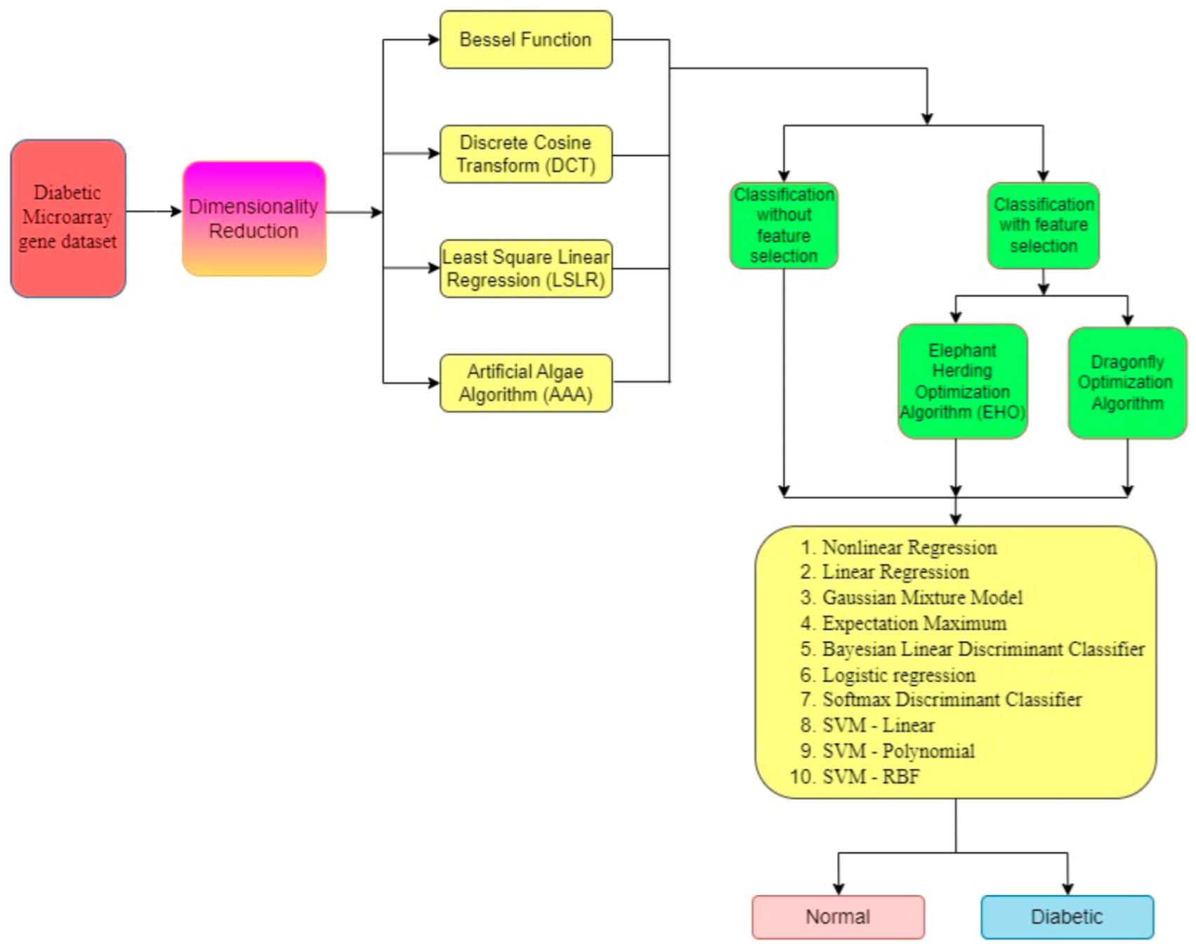
- The work suggests a novel approach for the early detection and diagnosis of diabetes using microarray gene expression data from pancreatic sources.
- Four DR techniques are used to reduce the high dimensionality of the microarray gene data.
- Two metaheuristic algorithms are used for feature selection to further reduce the dimensionality of the microarray gene data.
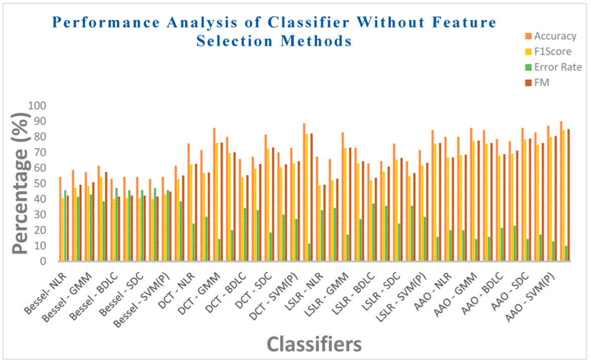
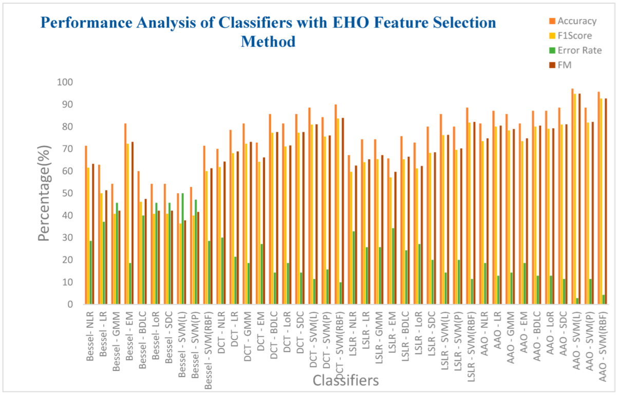
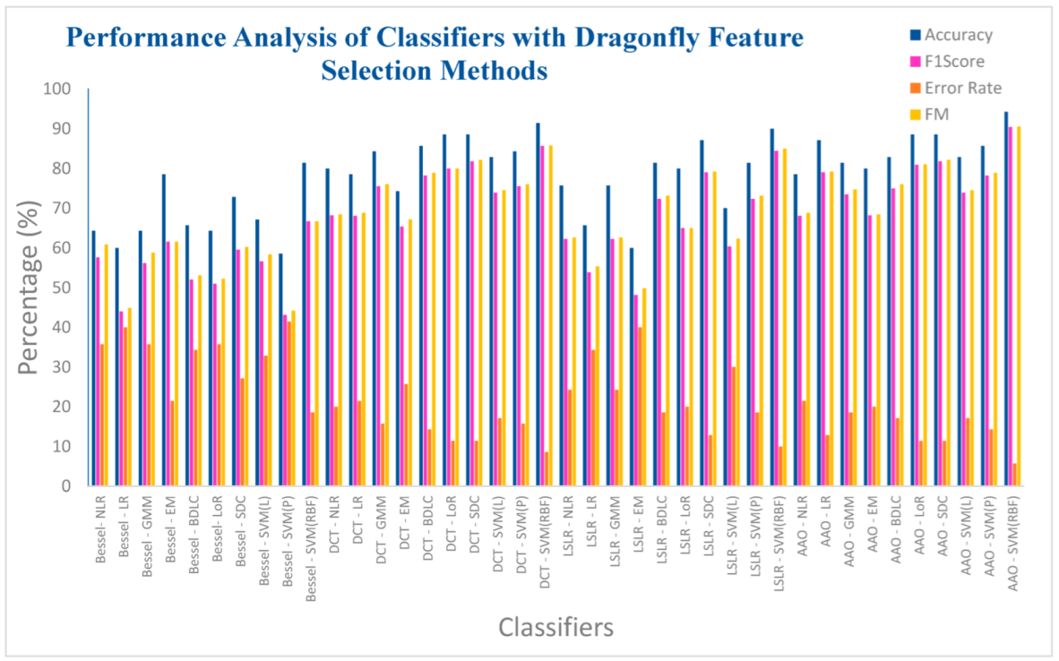
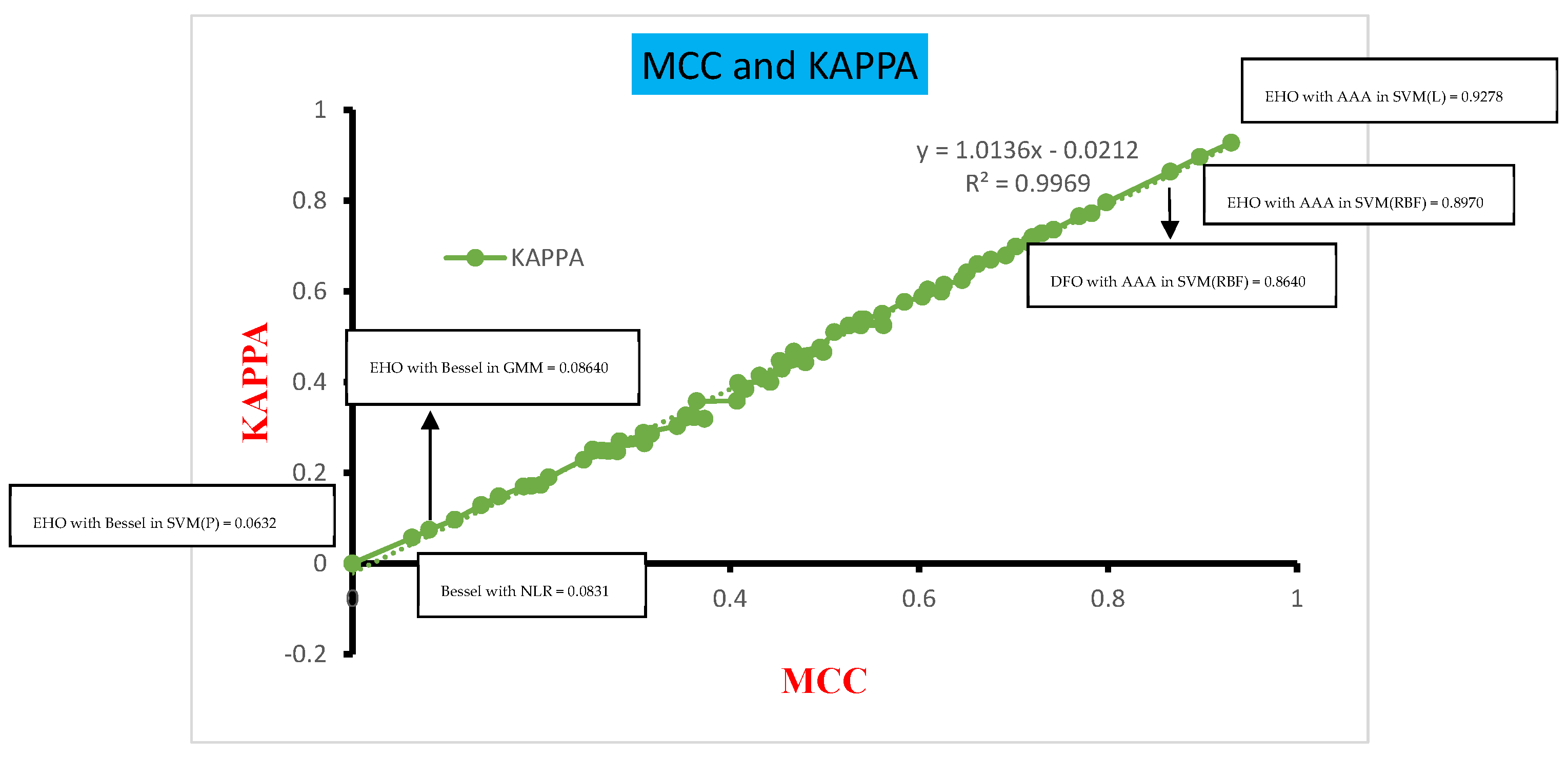
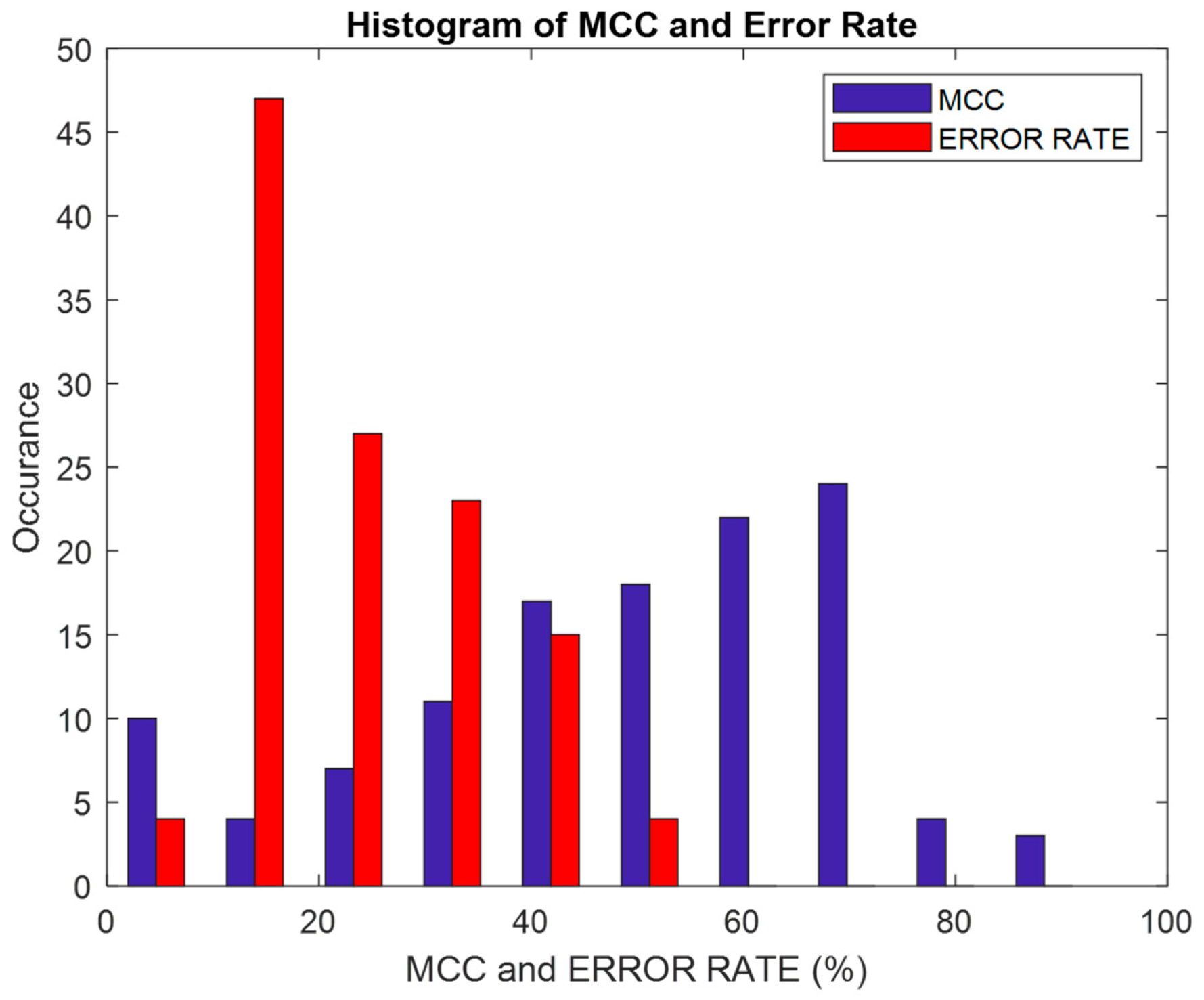
- Ten classifiers in two categories, namely nonlinear models and learning-based classifiers, are used to detect diabetes mellitus. The performance of the classifiers is analyzed based on parameters like accuracy, F1 score, MCC, error rate, FM metric, and Kappa, both with and without feature selection techniques. The enhancement of classifier performance due to feature selection is exemplified through MCC and Kappa plots.
3. Methodology
Role of Microarray Gene Data
4. Materials and Methods
Dataset
5. Need for Dimensionality Reduction Techniques
5.1. Dimensionality Reduction
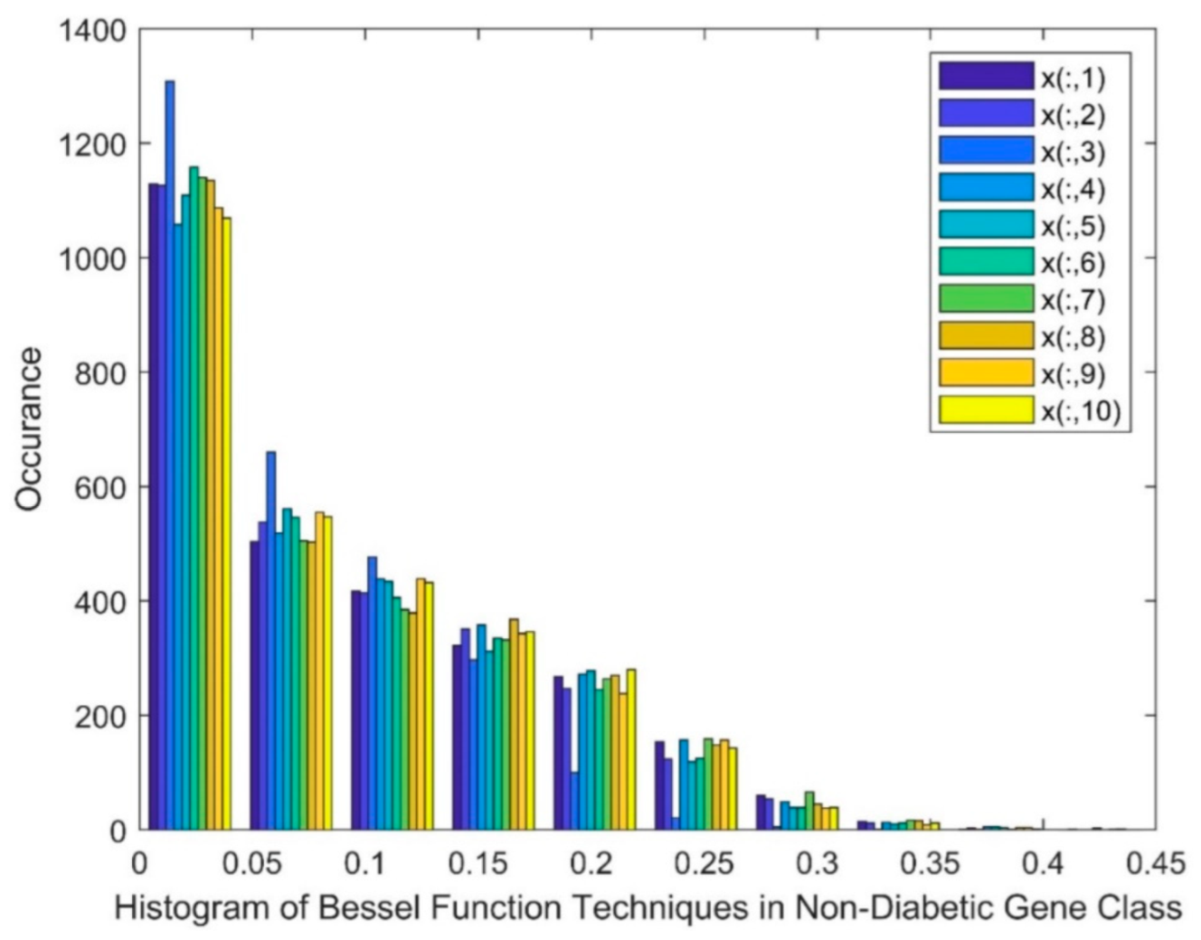
- Bessel Function as Dimensionality Reduction
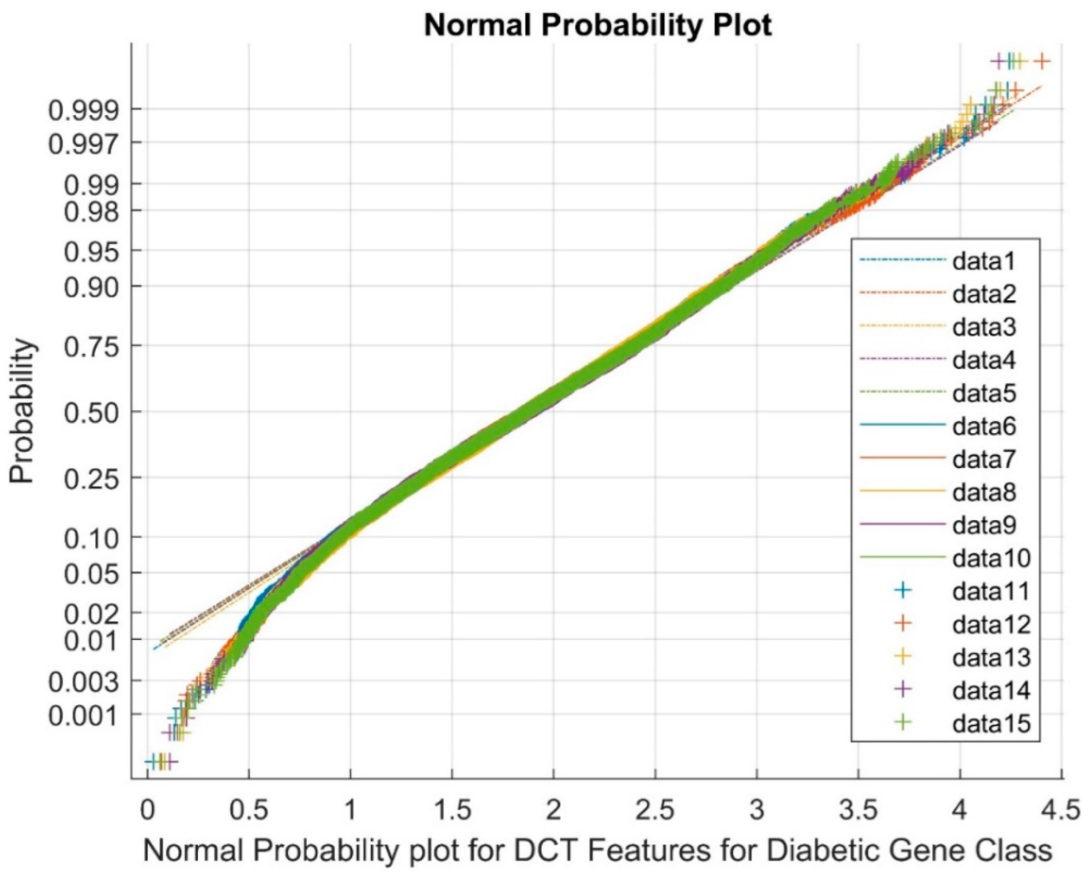
- DCT—Discrete Cosine Transform
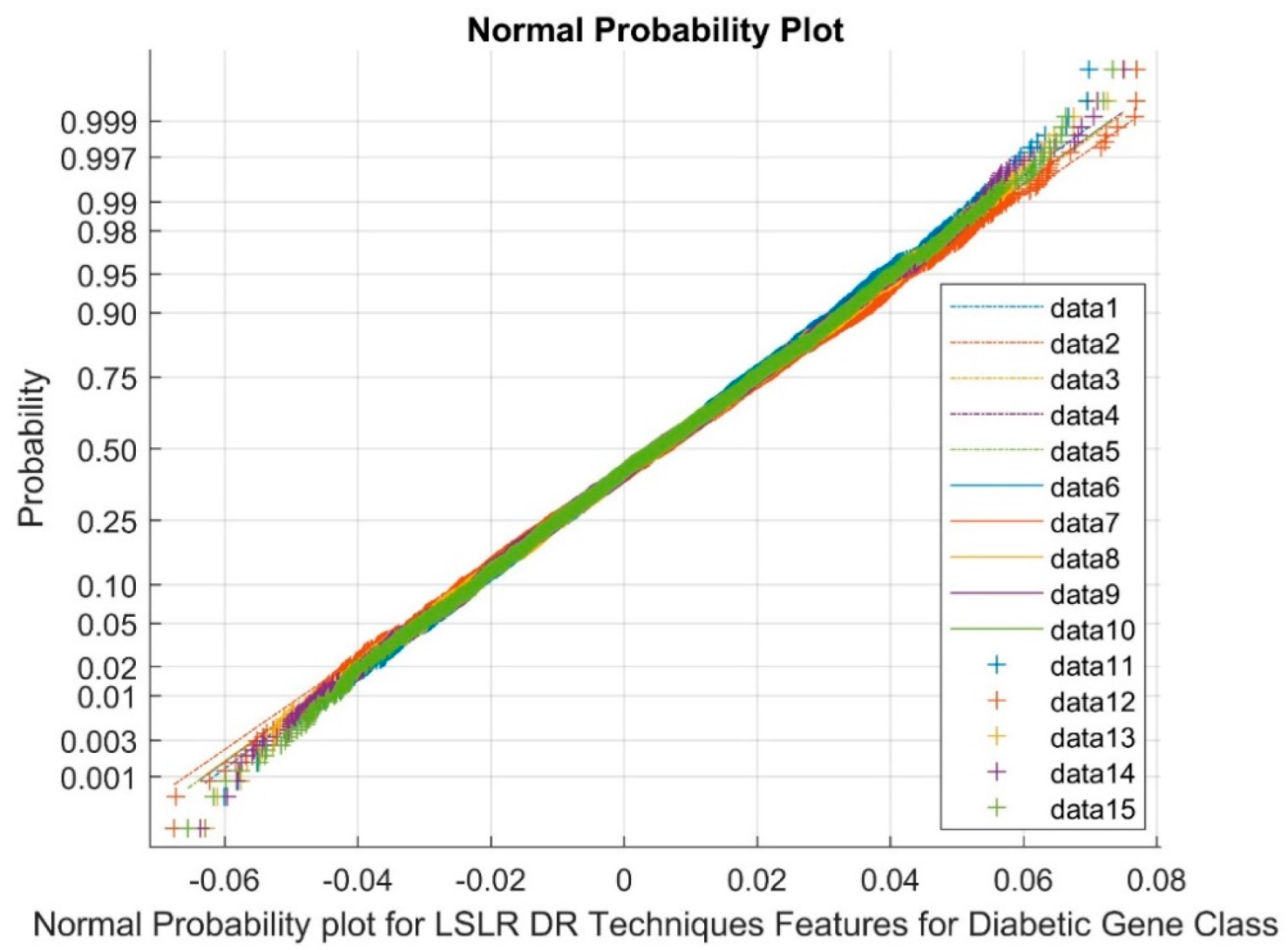
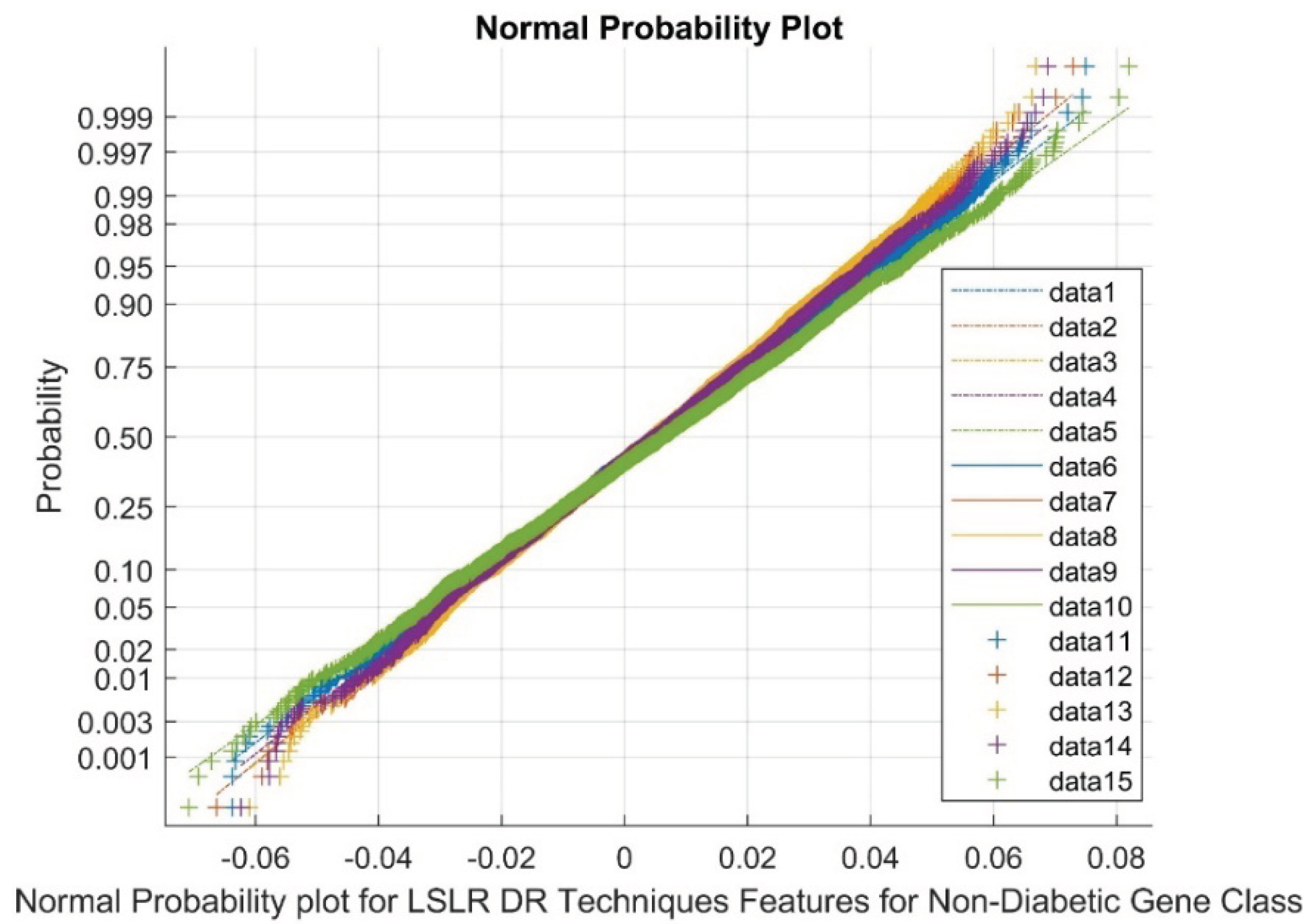
- Least Squares Linear Regression (LSLR) as Dimensionality Reduction
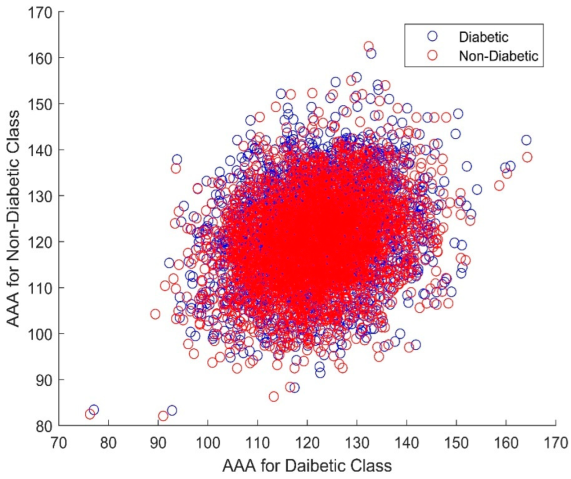
- Artificial Algae Algorithm (AAA) as Dimensionality Reduction
5.2. Statistical Analysis
6. Feature Selection Methods
- Elephant Herding Optimization (EHO) algorithm
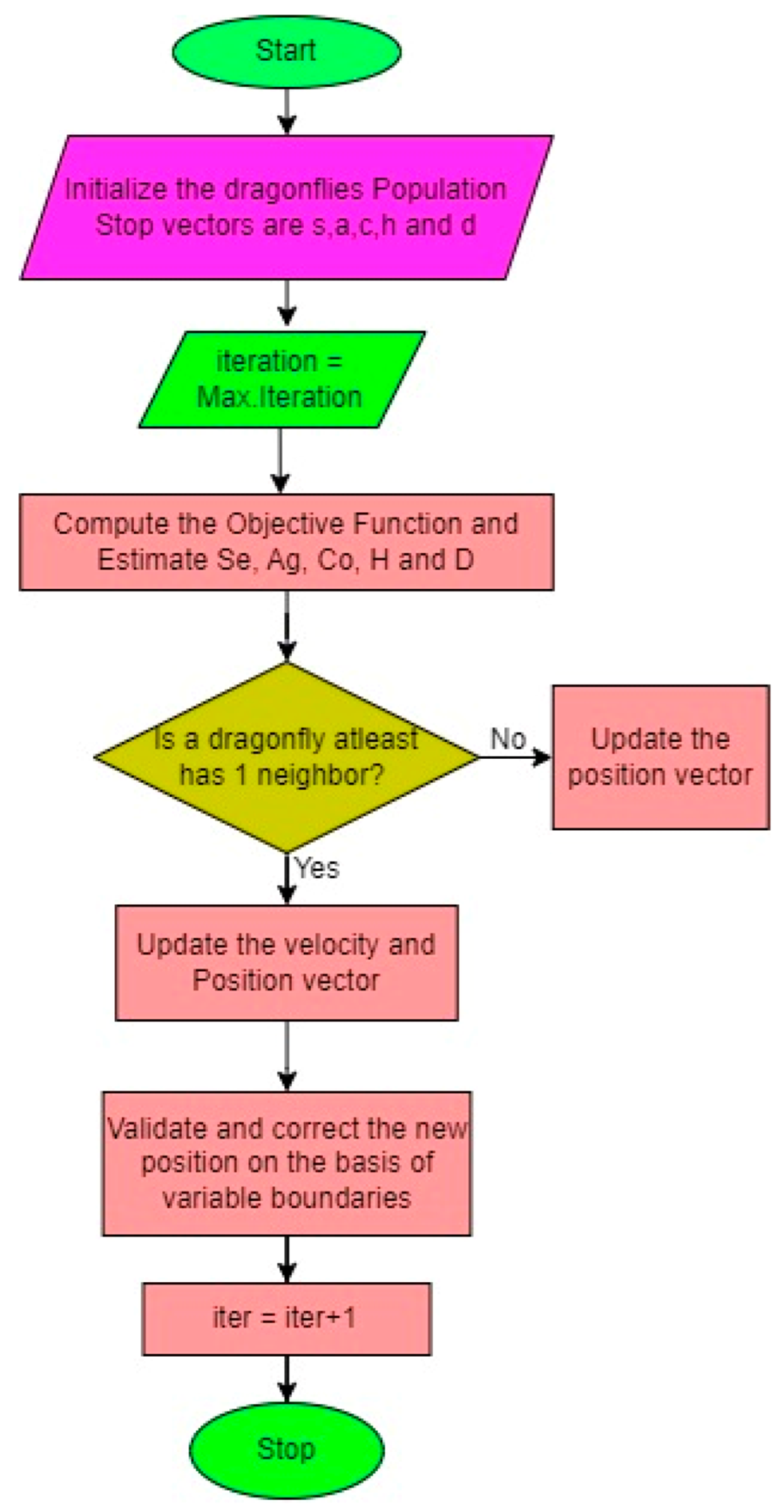
- Dragonfly Optimization Algorithm (DOA)
7. Classification Techniques
- NLR—Nonlinear Regression
- Linear Regression (LR)
- Gaussian Mixture Model (GMM)
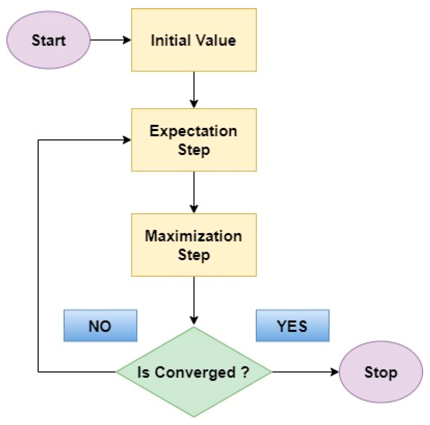
- Expectation Maximum (EM)
- Bayesian Linear Discriminant Classifier (BLDC)
- Logistic Regression (LoR)
- SDC—Softmax Discriminant Classifier
- Support Vector Machines
7.1. Training and Testing of Classifiers

| Clinical Situation | Predicted Values | ||
|---|---|---|---|
| Diabetic | Non-Diabetic | ||
| Real Values | Diabetic class | TP | FN |
| Non-diabetic class | FP | TN | |
7.2. Selection of Target
8. Results and Findings
8.1. Computational Complexity (CC)
8.2. Limitations and Major Outcomes
9. Conclusions
Author Contributions
Funding
Institutional Review Board Statement
Informed Consent Statement
Data Availability Statement
Conflicts of Interest
References
- Facts & Figures. International Diabetes Federation. Available online: https://idf.org/about-diabetes/facts-figures/ (accessed on 20 August 2021).
- Pradeepa, R.; Mohan, V. Epidemiology of type 2 diabetes in India. Indian J. Ophthalmol. 2021, 69, 2932–2938. [Google Scholar] [CrossRef]
- Chockalingam, S.; Aluru, M.; Aluru, S. Microarray data processing techniques for genome-scale network inference from large public repositories. Microarrays 2016, 5, 23. [Google Scholar] [CrossRef]
- Herman, W.H.; Ye, W.; Griffin, S.J.; Simmons, R.K.; Davies, M.J.; Khunti, K.; Wareham, N.J. Early detection and treatment of type 2 diabetes reduce cardiovascular morbidity and mortality: A simulation of the results of the Anglo-Danish-Dutch study of intensive treatment in people with screen-detected diabetes in primary care (ADDITION-Europe). Diabetes Care 2015, 38, 1449–1455. [Google Scholar] [CrossRef]
- Strianese, O.; Rizzo, F.; Ciccarelli, M.; Galasso, G.; D’Agostino, Y.; Salvati, A.; Rusciano, M.R. Precision and personalized medicine: How genomic approach improves the management of cardiovascular and neurodegenerative disease. Genes 2020, 11, 747. [Google Scholar] [CrossRef] [PubMed]
- Abul-Husn, N.S.; Kenny, E.E. Personalized medicine and the power of electronic health records. Cell 2019, 177, 58–69. [Google Scholar] [CrossRef] [PubMed]
- Schnell, O.; Crocker, J.B.; Weng, J. Impact of HbA1c testing at point of care on diabetes management. J. Diabetes Sci. Technol. 2017, 11, 611–617. [Google Scholar] [CrossRef]
- Lu, H.; Chen, J.; Yan, K.; Jin, Q.; Xue, Y.; Gao, Z. A hybrid feature selection algorithm for gene expression data classification. Neurocomputing 2017, 256, 56–62. [Google Scholar] [CrossRef]
- American Diabetes Association Professional Practice Committee. 2. Classification and Diagnosis of Diabetes: Standards of Medical Care in Diabetes—2022. Diabetes Care 2022, 45 (Suppl. S1), S17–S38. [Google Scholar] [CrossRef]
- Jakka, A.; Jakka, V.R. Performance evaluation of machine learning models for diabetes prediction. Int. J. Innov. Technol. Explor. Eng. Regul. Issue 2019, 8, 1976–1980. [Google Scholar] [CrossRef]
- Radja, M.; Emanuel, A.W.R. Performance evaluation of supervised machine learning algorithms using different data set sizes for diabetes prediction. In Proceedings of the 2019 5th International Conference on Science in Information Technology (ICSITech), Jogjakarta, Indonesia, 23–24 October 2019. [Google Scholar] [CrossRef]
- Dinh, A.; Miertschin, S.; Young, A.; Mohanty, S.D. A data-driven approach to predicting diabetes and cardiovascular disease with machine learning. BMC Med. Inform. Decis. Mak. 2019, 19, 211. [Google Scholar] [CrossRef]
- Yang, T.; Zhang, L.; Yi, L.; Feng, H.; Li, S.; Chen, H.; Zhu, J.; Zhao, J.; Zeng, Y.; Liu, H.; et al. Ensemble learning models based on noninvasive features for type 2 diabetes screening: Model development and validation. JMIR Med. Inform. 2020, 8, e15431. [Google Scholar] [CrossRef]
- Muhammad, L.J.; Algehyne, E.A.; Usman, S.S. Predictive supervised machine learning models for diabetes mellitus. SN Comput. Sci. 2020, 1, 240. [Google Scholar] [CrossRef]
- Kim, H.; Lim, D.H.; Kim, Y. Classification and prediction on the effects of nutritional intake on overweight/obesity, dyslipidemia, hypertension and type 2 diabetes mellitus using deep learning model: 4–7th Korea national health and nutrition examination survey. Int. J. Environ. Res. Public Health 2021, 18, 5597. [Google Scholar] [CrossRef] [PubMed]
- Lawi, A.; Syarif, S. Performance evaluation of naive Bayes and support vector machine in type 2 diabetes Mellitus gene expression microarray data. In Journal of Physics: Conference Series; IOP Publishing: Bristol, UK, 2019; Volume 1341, p. 042018. [Google Scholar]
- Ciaramella, A.; Staiano, A. On the role of clustering and visualization techniques in gene microarray data. Algorithms 2019, 12, 123. [Google Scholar] [CrossRef]
- Velliangiri, S.; Alagumuthukrishnan, S.; Joseph, S.I.T. A review of dimensionality reduction techniques for efficient computation. Procedia Comput. Sci. 2019, 165, 104–111. [Google Scholar] [CrossRef]
- Parand, K.; Nikarya, M. New numerical method based on generalized Bessel function to solve nonlinear Abel fractional differential equation of the first kind. Nonlinear Eng. 2019, 8, 438–448. [Google Scholar] [CrossRef]
- Bell, W.W. Special Functions for Scientists and Engineers; Courier Corporation: North Chelmsford, MA, USA, 1967. [Google Scholar]
- Kalaiyarasi, M.; Rajaguru, H. Performance Analysis of Ovarian Cancer Detection and Classification for Microarray Gene Data. BioMed Res. Int. 2022, 2022, 6750457. [Google Scholar] [CrossRef]
- Ahmed, N.; Natarajan, T.; Rao, K.R. Discrete cosine transform. IEEE Trans. Comput. 1974, C-23, 90–93. [Google Scholar] [CrossRef]
- Epps, J.; Ambikairajah, E. Use of the discrete cosine transform for gene expression data analysis. In Proceedings of the Workshop on Genomic Signal Processing and Statistics, Baltimore, MD, USA, 26–27 May 2004; Volume 1. [Google Scholar]
- Hotelling, H. Analysis of a complex of statistical variables into principal components. J. Educ. Psychol. 1933, 24, 417–441. [Google Scholar] [CrossRef]
- Hastie, T.; Tibshirani, R.; Friedman, J.H.; Friedman, J.H. The Elements of Statistical Learning: Data Mining, Inference, and Prediction; Springer: New York, NY, USA, 2009; Volume 2. [Google Scholar]
- Uymaz, S.A.; Tezel, G.; Yel, E. Artificial algae algorithm (AAA) for nonlinear global optimization. Appl. Soft Comput. 2015, 31, 153–171. [Google Scholar] [CrossRef]
- Prabhakar, S.K.; Lee, S.W. An integrated approach for ovarian cancer classification with the application of stochastic optimization. IEEE Access 2020, 8, 127866–127882. [Google Scholar] [CrossRef]
- Parhi, P.; Bisoi, R.; Dash, P.K. Influential gene selection from high-dimensional genomic data using a bio-inspired algorithm wrapped broad learning system. IEEE Access 2022, 10, 49219–49232. [Google Scholar] [CrossRef]
- Ewees, A.A.; Al-Qaness, M.A.; Abualigah, L.; Algamal, Z.Y.; Oliva, D.; Yousri, D.; Elaziz, M.A. Enhanced feature selection technique using slime mould algorithm: A case study on chemical data. Neural Comput. Appl. 2023, 35, 3307–3324. [Google Scholar] [CrossRef] [PubMed]
- Wang, G.G. Moth search algorithm: A bio-inspired metaheuristic algorithm for global optimization problems. Memetic Comput. 2018, 10, 151–164. [Google Scholar] [CrossRef]
- Lin, Y.; Heidari, A.A.; Wang, S.; Chen, H.; Zhang, Y. An Enhanced Hunger Games Search Optimization with Application to Constrained Engineering Optimization Problems. Biomimetics 2023, 8, 441. [Google Scholar] [CrossRef]
- Qiao, Z.; Li, L.; Zhao, X.; Liu, L.; Zhang, Q.; Hechmi, S.; Atri, M.; Li, X. An enhanced Runge Kutta boosted machine learning framework for medical diagnosis. Comput. Biol. Med. 2023, 160, 106949. [Google Scholar] [CrossRef] [PubMed]
- He, X.; Shan, W.; Zhang, R.; Heidari, A.A.; Chen, H.; Zhang, Y. Improved Colony Predation Algorithm Optimized Convolutional Neural Networks for Electrocardiogram Signal Classification. Biomimetics 2023, 8, 268. [Google Scholar] [CrossRef] [PubMed]
- Izci, D.; Ekinci, S.; Eker, E.; Demirören, A. Biomedical application of a random learning and elite opposition-based weighted mean of vectors algorithm with pattern search mechanism. J. Control. Autom. Electr. Syst. 2023, 34, 333–343. [Google Scholar] [CrossRef]
- Peng, L.; Cai, Z.; Heidari, A.A.; Zhang, L.; Chen, H. Hierarchical Harris hawks optimizer for feature selection. J. Adv. Res. 2023. [Google Scholar] [CrossRef]
- Su, H.; Zhao, D.; Heidari, A.A.; Liu, L.; Zhang, X.; Mafarja, M.; Chen, H. RIME: A physics-based optimization. Neurocomputing 2023, 532, 183–214. [Google Scholar] [CrossRef]
- Wang, G.G.; Deb, S.; Coelho, L.D.S. Elephant herding optimization. In Proceedings of the 2015 3rd International Symposium on Computational and Business Intelligence (ISCBI), Bali, Indonesia, 9 December 2015; IEEE: Piscataway, NJ, USA, 2015; pp. 1–5. [Google Scholar]
- Mirjalili, S. Dragonfly algorithm: A new meta-heuristic optimization technique for solving single-objective, discrete, and multi-objective problems. Neural Comput. Appl. 2016, 27, 1053–1073. [Google Scholar] [CrossRef]
- Bharanidharan, N.; Rajaguru, H. Dementia MRI image classification using transformation technique based on elephant herding optimization with Randomized Adam method for updating the hyper-parameters. Int. J. Imaging Syst. Technol. 2021, 31, 1221–1245. [Google Scholar] [CrossRef]
- Bharanidharan, N.; Rajaguru, H. Performance enhancement of swarm intelligence techniques in dementia classification using dragonfly-based hybrid algorithms. Int. J. Imaging Syst. Technol. 2020, 30, 57–74. [Google Scholar] [CrossRef]
- Zhang, G.; Allaire, D.; Cagan, J. Reducing the Search Space for Global Minimum: A Focused Regions Identification Method for Least Squares Parameter Estimation in Nonlinear Models. J. Comput. Inf. Sci. Eng. 2023, 23, 021006. [Google Scholar] [CrossRef]
- Draper, N.R.; Smith, H. Applied Regression Analysis; John Wiley & Sons: Hoboken, NJ, USA, 1998; Volume 326. [Google Scholar]
- Llaha, O.; Rista, A. Prediction and Detection of Diabetes using Machine Learning. In Proceedings of the 20th International Conference on Real-Time Applications in Computer Science and Information Technology (RTA-CSIT), Tirana, Albania, 21–22 May 2021; pp. 94–102. [Google Scholar]
- Prabhakar, S.K.; Rajaguru, H.; Lee, S.-W. A comprehensive analysis of alcoholic EEG signals with detrend fluctuation analysis and post classifiers. In Proceedings of the 2019 7th International Winter Conference on Brain-Computer Interface (BCI), Gangwon, Republic of Korea, 18–20 February 2019; IEEE: Piscataway, NJ, USA, 2019. [Google Scholar]
- Liu, S.; Zhang, X.; Xu, L.; Ding, F. Expectation–maximization algorithm for bilinear systems by using the Rauch–Tung–Striebel smoother. Automatica 2022, 142, 110365. [Google Scholar] [CrossRef]
- Zhou, W.; Liu, Y.; Yuan, Q.; Li, X. Epileptic seizure detection using lacunarity and Bayesian linear discriminant analysis in intracranial EEG. IEEE Trans. Biomed. Eng. 2013, 60, 3375–3381. [Google Scholar] [CrossRef]
- Hamid, I.Y. Prediction of Type 2 Diabetes through Risk Factors using Binary Logistic Regression. J. Al-Qadisiyah Comput. Sci. Math. 2020, 12, 1–11. [Google Scholar] [CrossRef]
- Adiwijaya, K.; Wisesty, U.N.; Lisnawati, E.; Aditsania, A.; Kusumo, D.S. Dimensionality reduction using principal component analysis for cancer detection based on microarray data classification. J. Comput. Sci. 2018, 14, 1521–1530. [Google Scholar] [CrossRef]
- Zang, F.; Zhang, J.S. Softmax Discriminant Classifier. In Proceedings of the 3rd International Conference on Multimedia Information Networking and Security, Shanghai, China, 4–6 November 2011; pp. 16–20. [Google Scholar]
- Yao, X.J.; Panaye, A.; Doucet, J.; Chen, H.; Zhang, R.; Fan, B.; Liu, M.; Hu, Z. Comparative classification study of toxicity mechanisms using support vector machines and radial basis function neural networks. Anal. Chim. Acta 2005, 535, 259–273. [Google Scholar] [CrossRef]
- Fushiki, T. Estimation of prediction error by using K-fold cross-validation. Stat. Comput. 2011, 21, 137–146. [Google Scholar] [CrossRef]
- Wang, Z.; Bovik, A.C. Mean squared error: Love it or leave it? A new look at signal fidelity measures. IEEE Signal Process. Mag. 2009, 26, 98–117. [Google Scholar] [CrossRef]
- Maniruzzaman, M.; Kumar, N.; Abedin, M.M.; Islam, M.S.; Suri, H.S.; El-Baz, A.S.; Suri, J.S. Comparative approaches for classification of diabetes mellitus data: Machine learning paradigm. Comput. Methods Programs Biomed. 2017, 152, 23–34. [Google Scholar] [CrossRef] [PubMed]
- Pham, T.; Tran, T.; Phung, D.; Venkatesh, S. Predicting healthcare trajectories from medical records: A deep learning approach. J. Biomed. Inform. 2017, 69, 218–229. [Google Scholar] [CrossRef] [PubMed]
- Hertroijs, D.F.L.; Elissen, A.M.J.; Brouwers, M.C.G.J.; Schaper, N.C.; Köhler, S.; Popa, M.C.; Asteriadis, S.; Hendriks, S.H.; Bilo, H.J.; Ruwaard, D.; et al. A risk score including body mass index, glycated hemoglobin and triglycerides predicts future glycemic control in people with type 2 diabetes. Diabetes Obes. Metab. 2017, 20, 681–688. [Google Scholar] [CrossRef]
- Arellano-Campos, O.; Gómez-Velasco, D.V.; Bello-Chavolla, O.Y.; Cruz-Bautista, I.; Melgarejo-Hernandez, M.A.; Muñoz-Hernandez, L.; Guillén, L.E.; Garduño-Garcia, J.D.J.; Alvirde, U.; Ono-Yoshikawa, Y.; et al. Development and validation of a predictive model for incident type 2 diabetes in middleaged Mexican adults: The metabolic syndrome cohort. BMC Endocr. Disord. 2019, 19, 41. [Google Scholar] [CrossRef]
- Deo, R.; Panigrahi, S. Performance assessment of machine learning based models for diabetes prediction. In Proceedings of the 2019 IEEE Healthcare Innovations and Point of Care Technologies, (HI-POCT), Bethesda, MD, USA, 20–22 November 2019. [Google Scholar] [CrossRef]
- Choi, B.G.; Rha, S.-W.; Kim, S.W.; Kang, J.H.; Park, J.Y.; Noh, Y.-K. Machine learning for the prediction of new-onset diabetes mellitus during 5-year follow-up in non-diabetic patients with cardiovascular risks. Yonsei Med. J. 2019, 60, 191. [Google Scholar] [CrossRef]
- Akula, R.; Nguyen, N.; Garibay, I. Supervised machine learning based ensemble model for accurate prediction of type 2 diabetes. In Proceedings of the 2019 Southeast Conference, Huntsville, AL, USA, 11–14 April 2019. [Google Scholar] [CrossRef]
- Xie, Z.; Nikolayeva, O.; Luo, J.; Li, D. Building risk prediction models for type 2 diabetes using machine learning techniques. Prev. Chronic Dis. 2019, 16, E130. [Google Scholar] [CrossRef]
- Bernardini, M.; Morettini, M.; Romeo, L.; Frontoni, E.; Burattini, L. Early temporal prediction of type 2 diabetes risk condition from a general practitioner electronic health record: A multiple instance boosting approach. Artif. Intell. Med. 2020, 105, 101847. [Google Scholar] [CrossRef]
- Zhang, L.; Wang, Y.; Niu, M.; Wang, C.; Wang, Z. Machine learning for characterizing risk of type 2 diabetes mellitus in a rural Chinese population: The Henan rural cohort study. Sci. Rep. 2020, 10, 4406. [Google Scholar] [CrossRef]
- Jain, S. A supervised model for diabetes divination. Biosci. Biotechnol. Res. Commun. 2020, 13 (Suppl. S14), 315–318. [Google Scholar] [CrossRef]
- Kalagotla, S.K.; Gangashetty, S.V.; Giridhar, K. A novel stacking technique for prediction of diabetes. Comput. Biol. Med. 2021, 135, 104554. [Google Scholar] [CrossRef]
- Haneef, R.; Fuentes, S.; Fosse-Edorh, S.; Hrzic, R.; Kab, S.; Cosson, E.; Gallay, A. Use of artifcial intelligence for public health surveillance: A case study to develop a machine learning-algorithm to estimate the incidence of diabetes mellitus in France. Arch. Public Health 2021, 79, 168. [Google Scholar] [CrossRef] [PubMed]
- Deberneh, H.M.; Kim, I. Prediction of Type 2 diabetes based on machine learning algorithm. Int. J. Environ. Res. Public Health 2021, 18, 3317. [Google Scholar] [CrossRef] [PubMed]
- Zhang, L.; Wang, Y.; Niu, M.; Wang, C.; Wang, Z. Nonlaboratory based risk assessment model for type 2 diabetes mellitus screening in Chinese rural population: A joint bagging boosting model. IEEE J. Biomed. Health Inform. 2021, 25, 4005–4016. [Google Scholar] [CrossRef] [PubMed]


| Type | Total Number | Diabetic Class | Non-Diabetic Class | Total Classes |
|---|---|---|---|---|
| Pancreatic dataset | 28,735 | 20 | 50 | 70 |
| Statistical Parameters | Bessel Function | Discrete Cosine Transform (DCT) | Least Squares Linear Regression (LSLR) | Artificial Algae Algorithm (AAA) | ||||
|---|---|---|---|---|---|---|---|---|
| Dia | Norm | Dia | Norm | Dia | Norm | Dia | Norm | |
| Mean | 0.082961 | 0.084162 | 1.882012 | 1.883618 | 0.00467 | 0.00457 | 121.664 | 120.5492 |
| Variance | 0.005165 | 0.005378 | 0.50819 | 0.506957 | 0.000432 | 0.000417 | 101.6366 | 103.0168 |
| Skewness | 0.865169 | 0.856162 | 0.187903 | 0.228924 | 0.003787 | −0.0315 | 0.042744 | 0.054472 |
| Kurtosis | 0.180926 | 0.135504 | −0.34524 | −0.40687 | −0.16576 | −0.08667 | 0.152272 | 0.091169 |
| Pearson CC | 0.866264 | 0.859211 | 0.98138 | 0.983118 | 0.975446 | 0.977318 | 0.9826 | 0.985246 |
| CCA | 0.05904 | 0.260275 | 0.090825 | 0.082321 | ||||
| Feature Selection | DR Techniques | Bessel Function | Discrete Cosine Transform (DCT) | Least Squares Linear Regression (LSLR) | Artificial Algae Algorithm (AAA) | ||||
|---|---|---|---|---|---|---|---|---|---|
| Genes | Dia | Norm | Dia | Norm | Dia | Norm | Dia | Norm | |
| EHO | p-value < 0.05 | 0.9721 | 0.9998 | 0.994 | 0.9996 | 0.9961 | 0.9999 | 0.9466 | 0.9605 |
| Dragonfly | p-value < 0.05 | 0.99985 | 0.876 | 0.9956 | 0.998 | 0.9951 | 0.99931 | 0.9936 | 0.9977 |
| Classifiers | Bessel Function | Discrete Cosine Transform (DCT) | Least Squares Linear Regression (LSLR) | Artificial Algae Algorithm (AAA) | ||||
|---|---|---|---|---|---|---|---|---|
| MSE Training Set | MSE Testing Set | MSE Training Set | MSE Testing Set | MSE Training Set | MSE Testing Set | MSE Training Set | MSE Testing Set | |
| NLR | 2.3 × 10⁻⁶ | 1.76 × 10⁻³ | 6.41 × 10⁻⁶ | 2.48 × 10⁻⁵ | 7.75 × 10⁻⁶ | 5.12 × 10⁻⁵ | 2.91 × 10⁻⁷ | 1.6 × 10⁻⁵ |
| LR | 2.41 × 10⁻⁵ | 9.51 × 10⁻⁵ | 7.52 × 10⁻⁶ | 3.11 × 10⁻⁵ | 2.18 × 10⁻⁷ | 4.66 × 10⁻⁵ | 3.67 × 10⁻⁸ | 1.45 × 10⁻⁵ |
| GMM | 2.1 × 10⁻⁵ | 1.75 × 10⁻⁴ | 5.72 × 10⁻⁷ | 6.8 × 10⁻⁶ | 3.09 × 10⁻⁷ | 1.11 × 10⁻⁵ | 3.76 × 10⁻⁶ | 5.33 × 10⁻⁵ |
| EM | 1.62 × 10⁻⁷ | 9.87 × 10⁻⁶ | 2.71 × 10⁻⁶ | 1.3 × 10⁻⁵ | 9.87 × 10⁻⁷ | 1.99 × 10⁻⁵ | 8.97 × 10⁻⁹ | 7.3 × 10⁻⁶ |
| BLDC | 1.4 × 10⁻⁶ | 2.53 × 10⁻³ | 2.86 × 10⁻⁷ | 3.94 × 10⁻⁵ | 4.74 × 10⁻⁶ | 5.28 × 10⁻⁵ | 1.43 × 10⁻⁷ | 1.64 × 10⁻⁵ |
| LoR | 1.2 × 10⁻⁶ | 2.89 × 10⁻³ | 9.47 × 10⁻⁶ | 3.58 × 10⁻⁵ | 8.69 × 10⁻⁶ | 4.54 × 10⁻⁵ | 9.26 × 10⁻⁸ | 1.45 × 10⁻⁵ |
| SDC | 1.9 × 10⁻⁶ | 2.03 × 10⁻³ | 3.66 × 10⁻⁶ | 1.07 × 10⁻⁵ | 2.47 × 10⁻⁶ | 1.86 × 10⁻⁵ | 2.31 × 10⁻⁹ | 5 × 10⁻⁶ |
| SVM (L) | 3.1 × 10⁻⁶ | 2.7 × 10⁻³ | 8.92 × 10⁻⁶ | 2.89 × 10⁻⁵ | 1.09 × 10⁻⁵ | 4.01 × 10⁻⁵ | 4.13 × 10⁻⁹ | 8.2 × 10⁻⁶ |
| SVM (Poly) | 3.6 × 10⁻⁵ | 2.11 × 10⁻³ | 3.36 × 10⁻⁶ | 2.11 × 10⁻⁵ | 1.29 × 10⁻⁶ | 2.85 × 10⁻⁵ | 7.84 × 10⁻⁹ | 4.69 × 10⁻⁶ |
| SVM (RBF) | 4.16 × 10⁻⁷ | 8.3 × 10⁻⁵ | 1.57 × 10⁻⁸ | 2.41 × 10⁻⁶ | 3.22 × 10⁻⁸ | 5.64 × 10⁻⁶ | 1.93 × 10⁻¹⁰ | 1.77 × 10⁻⁸ |
| Classifiers | Bessel Function | Discrete Cosine Transform (DCT) | Least Squares Linear Regression (LSLR) | Artificial Algae Algorithm (AAA) | ||||
|---|---|---|---|---|---|---|---|---|
| Training MSE | Testing MSE | Training MSE | Testing MSE | Training MSE | Testing MSE | Training MSE | Testing MSE | |
| NLR | 4.85 × 10⁻⁶ | 2.64 × 10⁻⁵ | 4.13 × 10⁻⁵ | 2.88 × 10⁻⁵ | 1.21 × 10⁻⁶ | 3.64 × 10⁻⁵ | 7.21 × 10⁻⁷ | 9.53 × 10⁻⁶ |
| LR | 3.62 × 10⁻⁶ | 4.79 × 10⁻⁵ | 6.92 × 10⁻⁶ | 1.35 × 10⁻⁵ | 7.72 × 10⁻⁶ | 1.96 × 10⁻⁵ | 6.98 × 10⁻⁷ | 4.23 × 10⁻⁶ |
| GMM | 6.13 × 10⁻⁶ | 2.26 × 10⁻⁴ | 7.63 × 10⁻⁷ | 9.22 × 10⁻⁶ | 4.57 × 10⁻⁶ | 1.39 × 10⁻⁵ | 3.81 × 10⁻⁷ | 4.52 × 10⁻⁶ |
| EM | 2.19 × 10⁻⁷ | 1.2 × 10⁻⁶ | 4.39 × 10⁻⁶ | 2.25 × 10⁻⁵ | 4.81 × 10⁻⁶ | 3.92 × 10⁻⁵ | 4.67 × 10⁻⁷ | 1 × 10⁻⁵ |
| BLDC | 4.47 × 10⁻⁶ | 6.56 × 10⁻⁵ | 7.94 × 10⁻⁷ | 5.8 × 10⁻⁵ | 3.72 × 10⁻⁶ | 1.56 × 10⁻⁵ | 3.52 × 10⁻⁷ | 3.97 × 10⁻⁶ |
| LoR | 3.24 × 10⁻⁶ | 2.26 × 10⁻⁴ | 3.32 × 10⁻⁶ | 1.09 × 10⁻⁵ | 8.37 × 10⁻⁶ | 2.26 × 10⁻⁵ | 7.61 × 10⁻⁸ | 3.82 × 10⁻⁶ |
| SDC | 9.62 × 10⁻⁶ | 2.31 × 10⁻⁴ | 9.13 × 10⁻⁷ | 4.62 × 10⁻⁵ | 4.87 × 10⁻⁶ | 1.52 × 10⁻⁵ | 9.93 × 10⁻⁸ | 3.84 × 10⁻⁶ |
| SVM (L) | 4.12 × 10⁻⁵ | 5.29 × 10⁻⁴ | 8.47 × 10⁻⁷ | 4.16 × 10⁻⁶ | 1.93 × 10⁻⁸ | 9.61 × 10⁻⁶ | 1.67 × 10⁻⁸ | 3.81 × 10⁻⁶ |
| SVM (Poly) | 6.41 × 10⁻⁵ | 2.34 × 10⁻⁴ | 2.19 × 10⁻⁷ | 6.41 × 10⁻⁶ | 5.77 × 10⁻⁸ | 1.24 × 10⁻⁵ | 1.62 × 10⁻⁸ | 2.05 × 10⁻⁶ |
| SVM (RBF) | 3.72 × 10⁻⁷ | 2.56 × 10⁻⁵ | 6.17 × 10⁻⁸ | 1.35 × 10⁻⁶ | 6.79 × 10⁻⁹ | 2.42 × 10⁻⁶ | 1.99 × 10⁻¹⁰ | 2.5 × 10⁻⁸ |
| Classifiers | Bessel Function | Discrete Cosine Transform (DCT) | Least Squares Linear Regression (LSLR) | Artificial Algae Algorithm (AAA) | ||||
|---|---|---|---|---|---|---|---|---|
| Training MSE | Testing MSE | Training MSE | Testing MSE | Training MSE | Testing MSE | Training MSE | Testing MSE | |
| NLR | 3.62 × 10⁻⁶ | 4.54 × 10⁻⁵ | 4.16 × 10⁻⁶ | 1.36 × 10⁻⁵ | 8.21 × 10⁻⁶ | 2.72 × 10⁻⁵ | 3.86 × 10⁻⁶ | 1.28 × 10⁻⁵ |
| LR | 4.36 × 10⁻⁶ | 7.12 × 10⁻⁵ | 2.84 × 10⁻⁶ | 1.39 × 10⁻⁵ | 9.4 × 10⁻⁶ | 3.8 × 10⁻⁵ | 2.51 × 10⁻⁸ | 4.32 × 10⁻⁶ |
| GMM | 7.58 × 10⁻⁷ | 4.71 × 10⁻⁵ | 5.66 × 10⁻⁸ | 7.84 × 10⁻⁶ | 3.61 × 10⁻⁶ | 2.09 × 10⁻⁵ | 4.63 × 10⁻⁸ | 1.02 × 10⁻⁵ |
| EM | 4.79 × 10⁻⁷ | 3.31 × 10⁻⁵ | 3.79 × 10⁻⁸ | 1.68 × 10⁻⁵ | 5.33 × 10⁻⁶ | 6.12 × 10⁻⁵ | 3.43 × 10⁻⁸ | 1.46 × 10⁻⁵ |
| BLDC | 6.52 × 10⁻⁷ | 4.16 × 10⁻⁵ | 2.92 × 10⁻⁸ | 4.49 × 10⁻⁵ | 7.54 × 10⁻⁸ | 9.12 × 10⁻⁶ | 7.68 × 10⁻⁸ | 8.1 × 10⁻⁶ |
| LoR | 6.54 × 10⁻⁷ | 5.04 × 10⁻⁵ | 7.23 × 10⁻⁸ | 6.05 × 10⁻⁶ | 1.92 × 10⁻⁷ | 2.23 × 10⁻⁶ | 4.84 × 10⁻⁹ | 3.36 × 10⁻⁶ |
| SDC | 3.86 × 10⁻⁷ | 2.57 × 10⁻⁵ | 8.95 × 10⁻⁷ | 3.08 × 10⁻⁶ | 7.52 × 10⁻⁸ | 6.31 × 10⁻⁶ | 1.63 × 10⁻⁸ | 2.52 × 10⁻⁶ |
| SVM (L) | 5.42 × 10⁻⁷ | 3.51 × 10⁻⁵ | 8.45 × 10⁻⁷ | 1.03 × 10⁻⁵ | 1.41 × 10⁻⁷ | 2.83 × 10⁻⁵ | 1.95 × 10⁻⁷ | 1.7 × 10⁻⁶ |
| SVM (Poly) | 9.67 × 10⁻⁷ | 7.23 × 10⁻⁵ | 6.67 × 10⁻⁶ | 7.08 × 10⁻⁶ | 6.3 × 10⁻⁷ | 1.05 × 10⁻⁵ | 6.42 × 10⁻⁸ | 5.33 × 10⁻⁶ |
| SVM (RBF) | 8.64 × 10⁻⁸ | 2.72 × 10⁻⁶ | 1.82 × 10⁻⁸ | 9.05 × 10⁻⁷ | 3.4 × 10⁻⁸ | 1.69 × 10⁻⁶ | 1.66 × 10⁻⁸ | 3.25 × 10⁻⁸ |
| Classifiers | Description |
|---|---|
| NLR | Uniform weight w = 0.4, bias b = 0.001, iteratively modified sum of least square error, criterion: MSE |
| Linear Regression | Uniform weight w = 0.451, bias b = 0.003, criterion: MSE |
| GMM | Mean covariance of the input samples and tuning parameter using EM steps. Criterion: MSE |
| EM | 0.13 likelihood probability, 0.45 cluster probability, with convergence rate of 0.631. Condition: MSE |
| BDLC | P(y), prior probability: 0.5, class mean: 0.85, 0.1; criterion: MSE |
| Logistic regression | Threshold Hθ(x) < 0.48 with criterion: MSE |
| SDC | Γ = 0.5 along with mean of each class target values as 0.1 and 0.85 |
| SVM (Linear) | C (Regularization Parameter): 0.85, class weights: 0.4, convergence criterion: MSE |
| SVM (Polynomial) | C: 0.76, coefficient of the kernel function (gamma): 10, class weights: 0.5, convergence criterion: MSE |
| SVM (RBF) | C: 1, coefficient of the kernel function (gamma): 100, class weights: 0.86, convergence criterion: MSE |
| Metrics | Formula | Assessment Focus |
|---|---|---|
| Accuracy | Fraction of predictions that are correct | |
| F1 Score | Harmonic mean of precision and recall | |
| Matthews Correlation Coefficient (MCC) | Correlation between the observed and predicted classifications | |
| Error Rate | Fraction of predictions that are incorrect | |
| FM Metric | Generalization of the F-measure that adds a beta parameter | |
| Kappa | Statistic that measures agreement between observed and predicted classifications, adjusted for chance |
| Dimensionality Reduction | Classifiers | Parameters | |||||
|---|---|---|---|---|---|---|---|
| Accuracy (%) | F1 Score (%) | MCC | Error Rate (%) | FM (%) | Kappa | ||
| Bessel Function | NLR | 54.2857 | 40.7407 | 0.0813 | 45.7142 | 42.1831 | 0.0743 |
| LR | 58.5714 | 47.2727 | 0.1897 | 41.4285 | 49.1354 | 0.1714 | |
| GMM | 57.1428 | 48.2758 | 0.1995 | 42.8571 | 50.7833 | 0.1732 | |
| EM | 61.4285 | 54.2372 | 0.3092 | 38.5714 | 57.2892 | 0.2645 | |
| BLDC | 52.8571 | 40 | 0.0632 | 47.1428 | 41.5761 | 0.0571 | |
| LoR | 54.2857 | 40.7407 | 0.0813 | 45.7142 | 42.1831 | 0.0743 | |
| SDC | 54.2857 | 40.7407 | 0.0813 | 45.7142 | 42.1831 | 0.0743 | |
| SVM (L) | 52.8571 | 40 | 0.0632 | 47.1428 | 41.5761 | 0.0571 | |
| SVM (Poly) | 54.2857 | 42.8571 | 0.1084 | 45.7142 | 44.7214 | 0.0967 | |
| SVM (RBF) | 61.4285 | 52.6315 | 0.2805 | 38.5714 | 55.1411 | 0.2470 | |
| Discrete Cosine Transform (DCT) | NLR | 75.7142 | 62.2222 | 0.4525 | 24.2857 | 62.6099 | 0.4465 |
| LR | 71.4285 | 56.5217 | 0.3646 | 28.5714 | 57.0088 | 0.3577 | |
| GMM | 85.7142 | 76.1904 | 0.6617 | 14.2857 | 76.277 | 0.6601 | |
| EM | 80 | 69.5652 | 0.5609 | 20 | 70.1646 | 0.5504 | |
| BLDC | 65.7142 | 53.8461 | 0.3083 | 34.2857 | 55.3399 | 0.2881 | |
| LoR | 67.1428 | 59.6491 | 0.4072 | 32.8571 | 62.4932 | 0.3585 | |
| SDC | 81.4285 | 72.3404 | 0.6032 | 18.5714 | 73.1564 | 0.5882 | |
| SVM (L) | 70 | 60.3773 | 0.4162 | 30 | 62.2799 | 0.3849 | |
| SVM (Poly) | 72.8571 | 62.7451 | 0.4547 | 27.1428 | 64.2575 | 0.4291 | |
| SVM (RBF) | 88.5714 | 81.8181 | 0.7423 | 11.4285 | 82.1584 | 0.7358 | |
| Least Squares Linear Regression (LSLR) | NLR | 67.1428 | 48.8888 | 0.2545 | 32.8571 | 49.1935 | 0.2511 |
| LR | 65.7142 | 52 | 0.2829 | 34.2857 | 53.0723 | 0.2695 | |
| GMM | 82.8571 | 72.7272 | 0.6091 | 17.1428 | 73.0297 | 0.6037 | |
| EM | 72.8571 | 62.7451 | 0.4547 | 27.1428 | 64.2575 | 0.4291 | |
| BLDC | 62.8571 | 51.8518 | 0.2711 | 37.1428 | 53.6875 | 0.2479 | |
| LoR | 64.2857 | 57.6271 | 0.3728 | 35.7142 | 60.8698 | 0.3190 | |
| SDC | 75.7142 | 65.3061 | 0.4952 | 24.2857 | 66.4364 | 0.4757 | |
| SVM (L) | 64.2857 | 54.5454 | 0.3162 | 35.7142 | 56.6947 | 0.2857 | |
| SVM (Poly) | 71.4285 | 61.5384 | 0.4352 | 28.5714 | 63.2456 | 0.4067 | |
| SVM (RBF) | 84.2857 | 75.5555 | 0.6505 | 15.7142 | 76.0263 | 0.6418 | |
| Artificial Algae Algorithm (AAA) | NLR | 80 | 66.6666 | 0.5254 | 20 | 66.7424 | 0.5242 |
| LR | 80 | 68.1818 | 0.5424 | 20 | 68.4653 | 0.5377 | |
| GMM | 85.7142 | 77.2727 | 0.6757 | 14.2857 | 77.594 | 0.6698 | |
| EM | 84.2857 | 75.5555 | 0.6505 | 15.7142 | 76.0263 | 0.6418 | |
| BLDC | 78.5714 | 68.0851 | 0.5382 | 21.4285 | 68.853 | 0.5248 | |
| LoR | 77.1428 | 69.2307 | 0.5622 | 22.8571 | 71.1512 | 0.5254 | |
| SDC | 85.7142 | 78.2608 | 0.6918 | 14.2857 | 78.9352 | 0.6788 | |
| SVM (L) | 82.8571 | 75 | 0.6454 | 17.1428 | 76.0639 | 0.625 | |
| SVM (Poly) | 87.1428 | 80 | 0.7165 | 12.8571 | 80.4984 | 0.7069 | |
| SVM (RBF) | 90 | 84.4444 | 0.7825 | 10 | 84.9706 | 0.7720 | |
| Dimensionality Reduction | Classifiers | Parameters | |||||
|---|---|---|---|---|---|---|---|
| Accuracy (%) | F1 Score (%) | MCC | Error Rate (%) | FM (%) | Kappa | ||
| Bessel Function | NLR | 71.4285 | 61.5384 | 0.4352 | 28.5714 | 63.2456 | 0.4067 |
| LR | 62.8571 | 50 | 0.2448 | 37.1428 | 51.387 | 0.2288 | |
| GMM | 54.2857 | 40.7407 | 0.0813 | 45.7142 | 42.1831 | 0.0743 | |
| EM | 81.4285 | 72.3404 | 0.6032 | 18.5714 | 73.1564 | 0.5882 | |
| BLDC | 60 | 46.1538 | 0.1813 | 40 | 47.4342 | 0.1694 | |
| LoR | 54.2857 | 40.7407 | 0.0813 | 45.7142 | 42.1831 | 0.0743 | |
| SDC | 54.2857 | 40.7407 | 0.0813 | 45.7142 | 42.1831 | 0.0743 | |
| SVM (L) | 50 | 36.3636 | 0 | 50 | 37.7964 | 0 | |
| SVM (Poly) | 52.8571 | 40 | 0.0632 | 47.1428 | 41.5761 | 0.0571 | |
| SVM (RBF) | 71.4285 | 60 | 0.4107 | 28.5714 | 61.2372 | 0.3913 | |
| Discrete Cosine Transform (DCT) | NLR | 70 | 61.8181 | 0.4427 | 30 | 64.254 | 0.4 |
| LR | 78.5714 | 68.0851 | 0.5382 | 21.4285 | 68.853 | 0.5248 | |
| GMM | 81.4285 | 72.3404 | 0.6032 | 18.5714 | 73.1564 | 0.5882 | |
| EM | 72.8571 | 64.1509 | 0.4796 | 27.1428 | 66.1724 | 0.4435 | |
| BLDC | 85.7142 | 77.2727 | 0.6757 | 14.2857 | 77.594 | 0.6698 | |
| LoR | 81.4285 | 71.1111 | 0.5845 | 18.5714 | 71.5542 | 0.5767 | |
| SDC | 85.7142 | 77.2727 | 0.6757 | 14.2857 | 77.594 | 0.6698 | |
| SVM (L) | 88.5714 | 80.9523 | 0.7298 | 11.4285 | 81.0443 | 0.7281 | |
| SVM (Poly) | 84.2857 | 75.5555 | 0.6505 | 15.7142 | 76.0263 | 0.6418 | |
| SVM (RBF) | 90 | 83.7209 | 0.7694 | 10 | 83.9254 | 0.7655 | |
| Least Squares Linear Regression (LSLR) | NLR | 67.1428 | 59.6491 | 0.4072 | 32.8571 | 62.4932 | 0.3585 |
| LR | 74.2857 | 64 | 0.4746 | 25.7142 | 65.3197 | 0.4521 | |
| GMM | 74.2857 | 65.3846 | 0.4987 | 25.7142 | 67.1984 | 0.4661 | |
| EM | 65.7142 | 57.1428 | 0.3615 | 34.2857 | 59.6285 | 0.3225 | |
| BLDC | 75.7142 | 65.3061 | 0.4952 | 24.2857 | 66.4364 | 0.4757 | |
| LoR | 72.8571 | 61.2244 | 0.4310 | 27.1428 | 62.2841 | 0.4140 | |
| SDC | 80 | 68.1818 | 0.5424 | 20 | 68.4653 | 0.5377 | |
| SVM (L) | 85.7142 | 76.1904 | 0.6617 | 14.2857 | 76.277 | 0.6601 | |
| SVM (Poly) | 80 | 69.5652 | 0.5609 | 20 | 70.1646 | 0.5504 | |
| SVM (RBF) | 88.5714 | 81.8181 | 0.7423 | 11.4285 | 82.1584 | 0.7358 | |
| Artificial Algae Algorithm (AAA) | NLR | 81.4285 | 73.4693 | 0.6236 | 18.5714 | 74.7409 | 0.5991 |
| LR | 87.1428 | 80 | 0.7165 | 12.8571 | 80.4984 | 0.7069 | |
| GMM | 85.7142 | 78.2608 | 0.6918 | 14.2857 | 78.9352 | 0.6788 | |
| EM | 81.4285 | 73.4693 | 0.6236 | 18.5714 | 74.7409 | 0.5991 | |
| BLDC | 87.1428 | 80 | 0.7165 | 12.8571 | 80.4984 | 0.7069 | |
| LoR | 87.1428 | 79.0697 | 0.7021 | 12.8571 | 79.2629 | 0.6985 | |
| SDC | 88.5714 | 80.9523 | 0.7298 | 11.4285 | 81.0443 | 0.7281 | |
| SVM (L) | 97.1428 | 94.7368 | 0.9302 | 2.85714 | 94.8683 | 0.9278 | |
| SVM (Poly) | 88.5714 | 81.8181 | 0.7423 | 11.4285 | 82.1584 | 0.7358 | |
| SVM (RBF) | 95.7142 | 92.6829 | 0.8970 | 4.28571 | 92.7105 | 0.8965 | |
| DR | Classifiers | Parameters | |||||
|---|---|---|---|---|---|---|---|
| Accuracy (%) | F1 Score (%) | MCC | Error Rate (%) | FM (%) | Kappa | ||
| Bessel Function | NLR | 64.2857 | 57.6271 | 0.3728 | 35.7142 | 60.8698 | 0.3190 |
| LR | 60 | 44 | 0.1551 | 40 | 44.9073 | 0.1478 | |
| GMM | 64.2857 | 56.1403 | 0.3438 | 35.7142 | 58.8172 | 0.3027 | |
| EM | 78.5714 | 61.5384 | 0.4673 | 21.4285 | 61.5587 | 0.4670 | |
| BLDC | 65.7142 | 52 | 0.2829 | 34.2857 | 53.0723 | 0.2695 | |
| LoR | 64.2857 | 50.9803 | 0.2637 | 35.7142 | 52.2093 | 0.2489 | |
| SDC | 72.8571 | 59.5744 | 0.4083 | 27.1428 | 60.2464 | 0.3981 | |
| SVM (L) | 67.1428 | 56.6037 | 0.3529 | 32.8571 | 58.3874 | 0.3263 | |
| SVM (Poly) | 58.5714 | 43.1372 | 0.1364 | 41.4285 | 44.1771 | 0.1287 | |
| SVM (RBF) | 81.4285 | 66.6666 | 0.5384 | 18.5714 | 66.6886 | 0.5380 | |
| Discrete Cosine Transform (DCT) | NLR | 80 | 68.1818 | 0.5424 | 20 | 68.4653 | 0.5377 |
| LR | 78.5714 | 68.0851 | 0.5382 | 21.4285 | 68.853 | 0.5248 | |
| GMM | 84.2857 | 75.5555 | 0.6505 | 15.7142 | 76.0263 | 0.6418 | |
| EM | 74.2857 | 65.3846 | 0.4987 | 25.7142 | 67.1984 | 0.4661 | |
| BLDC | 85.7142 | 78.2608 | 0.6918 | 14.2857 | 78.9352 | 0.6788 | |
| LoR | 88.5714 | 80 | 0.72 | 11.4285 | 80 | 0.72 | |
| SDC | 88.5714 | 81.8181 | 0.7423 | 11.4285 | 82.1584 | 0.7358 | |
| SVM (L) | 82.8571 | 73.9130 | 0.6264 | 17.1428 | 74.5499 | 0.6146 | |
| SVM (Poly) | 84.2857 | 75.5555 | 0.6505 | 15.7142 | 76.0263 | 0.6418 | |
| SVM (RBF) | 91.4285 | 85.7142 | 0.7979 | 8.57142 | 85.8116 | 0.7961 | |
| Least Squares Linear Regression (LSLR) | NLR | 75.7142 | 62.2222 | 0.4525 | 24.2857 | 62.6099 | 0.4465 |
| LR | 65.7142 | 53.8461 | 0.3083 | 34.2857 | 55.3399 | 0.2881 | |
| GMM | 75.7142 | 62.2222 | 0.4525 | 24.2857 | 62.6099 | 0.4465 | |
| EM | 60 | 48.1481 | 0.2078 | 40 | 49.8527 | 0.1900 | |
| BLDC | 81.4285 | 72.3404 | 0.6032 | 18.5714 | 73.1564 | 0.5882 | |
| LoR | 80 | 65 | 0.51 | 20 | 65 | 0.51 | |
| SDC | 87.1428 | 79.0697 | 0.7021 | 12.8571 | 79.2629 | 0.6985 | |
| SVM (L) | 70 | 60.3773 | 0.4162 | 30 | 62.2799 | 0.3849 | |
| SVM (Poly) | 81.4285 | 72.3404 | 0.6032 | 18.5714 | 73.1564 | 0.5882 | |
| SVM (RBF) | 90 | 84.4444 | 0.7825 | 10 | 84.9706 | 0.7720 | |
| Artificial Algae Algorithm (AAA) | NLR | 78.5714 | 68.0851 | 0.5382 | 21.4285 | 68.853 | 0.5248 |
| LR | 87.1428 | 79.0697 | 0.7021 | 12.8571 | 79.2629 | 0.6985 | |
| GMM | 81.4285 | 73.4693 | 0.6236 | 18.5714 | 74.7409 | 0.5991 | |
| EM | 80 | 68.1818 | 0.5424 | 20 | 68.4653 | 0.5377 | |
| BLDC | 82.8571 | 75 | 0.6454 | 17.1428 | 76.0639 | 0.625 | |
| LoR | 88.5714 | 80.9523 | 0.7298 | 11.4285 | 81.0443 | 0.7281 | |
| SDC | 88.5714 | 81.8181 | 0.7423 | 11.4285 | 82.1584 | 0.7358 | |
| SVM (L) | 82.8571 | 73.9130 | 0.6264 | 17.1428 | 74.5499 | 0.6146 | |
| SVM (Poly) | 85.7142 | 78.2608 | 0.6918 | 14.2857 | 78.9352 | 0.6788 | |
| SVM (RBF) | 94.2857 | 90.4761 | 0.8660 | 5.71428 | 90.5789 | 0.8640 | |
| Classifiers | DR Method | |||
|---|---|---|---|---|
| Bessel Function | Discrete Cosine Transform (DST) | Least Squares Linear Regression (LSLR) | Artificial Algae Algorithm (AAA) | |
| NLR | O(n2logn) | O(n2logn) | O(n3log2n) | O(n3log4n) |
| LR | O(n2logn) | O(n2logn) | O(n3log2n) | O(n3log4n) |
| GMM | O(n2log2n) | O(n2log2n) | O(n3log2n) | O(n3log4n) |
| EM | O(n3logn) | O(n3logn) | O(n3log2n) | O(n3log4n) |
| BLDC | O(n3logn) | O(n3logn) | O(2n3log2n) | O(2n3log4n) |
| LoR | O(2n2logn) | O(2n2logn) | O(2n4log2n) | O(2n4log4n) |
| SDC | O(n3logn) | O(n3logn) | O(n4log2n) | O(n4log4n) |
| SVM (L) | O(2n3logn) | O(2n3logn) | O(2n4log2n) | O(2n4log4n) |
| SVM (Poly) | O(2n3log2n) | O(2n3log2n) | O(2n4log4n) | O(2n4log8n) |
| SVM (RBF) | O(2n4log2n) | O(2n4log2n) | O(2n5log4n) | O(2n5log8n) |
| Classifiers | DR Method | |||
|---|---|---|---|---|
| Bessel Function | Discrete Cosine Transform (DCT) | Least Squares Linear Regression (LSLR) | Artificial Algae Algorithm (AAA) | |
| NLR | O(n4logn) | O(n4logn) | O(n5log2n) | O(n5log4n) |
| LR | O(n4logn) | O(n4logn) | O(n5log2n) | O(n5log4n) |
| GMM | O(n4log2n) | O(n4log2n) | O(n5log2n) | O(n5log4n) |
| EM | O(n5logn) | O(n5logn) | O(n5log2n) | O(n5log4n) |
| BLDC | O(n5logn) | O(n5logn) | O(2n5log2n) | O(2n5log4n) |
| LoR | O(2n4logn) | O(2n4logn) | O(2n5log2n) | O(2n5log4n) |
| SDC | O(n5logn) | O(n5logn) | O(n6log2n) | O(n6log4n) |
| SVM (L) | O(2n5logn) | O(2n5logn) | O(2n6log2n) | O(2n6log4n) |
| SVM (Poly) | O(2n5log2n) | O(2n5log2n) | O(2n6log4n) | O(2n6log8n) |
| SVM (RBF) | O(2n6log2n) | O(2n6log2n) | O(2n7log4n) | O(2n7log8n) |
| Classifiers | DR Method | |||
|---|---|---|---|---|
| Bessel Function | Discrete Cosine Transform (DST) | Least Squares Linear Regression (LSLR) | Artificial Algae Algorithm (AAA) | |
| NLR | O(4n3logn) | O(4n3logn) | O(4n4log2n) | O(4n4log4n) |
| LR | O(4n3logn) | O(4n3logn) | O(4n4log2n) | O(4n4log4n) |
| GMM | O(4n3log2n) | O(4n3log2n) | O(4n4log2n) | O(4n4log4n) |
| EM | O(4n4logn) | O(4n4logn) | O(4n4log2n) | O(4n4log4n) |
| BLDC | O(4n4logn) | O(4n4logn) | O(8n4log2n) | O(8n4log4n) |
| LoR | O(8n3logn) | O(8n3logn) | O(8n5log2n) | O(8n5log4n) |
| SDC | O(4n4logn) | O(4n4logn) | O(4n5log2n) | O(4n5log4n) |
| SVM (L) | O(8n4logn) | O(8n4logn) | O(8n5log2n) | O(8n5log4n) |
| SVM (Poly) | O(8n4log2n) | O(8n4log2n) | O(8n5log4n) | O(8n5log8n) |
| SVM (RBF) | O(8n5log2n) | O(8n5log2n) | O(8n6log4n) | O(8n6log8n) |
| S.No | Author (with Year) | Description of the Population | Data Sampling | Machine Learning Parameter | Accuracy (%) |
|---|---|---|---|---|---|
| 1. | Maniruzzaman et al., (2017) [53] | PIDD (Pima Indian diabetic dataset) | Cross-validation K2, K4, K5, K10, and JK | LDA, QDA, NB, GPC, SVM, ANN, AB, LoR, DT, RF | ACC: 92 |
| 2. | Pham et al., (2017) [54] | Diabetes: 12,000, aged between 18 and 100 Age (mean): 73 | Training set—66%; tuning set 17%; test set—17% | RNN, CLST Memory (C-LSTM) | ACC—79 |
| 3. | Hertroijs et al., (2018) [55] | Total: 105,814 Age (mean): greater than 18 | Training set of 90% and test set of 10% fivefold cross-validation | Latent Growth Mixture Modeling (LGMM) | ACC: 92.3 |
| 4. | ArellanoCampos et al., (2019) [56] | Base L: 7636 follow: 6144 diabetes: 331 age: 32–54 | K = 10, cross-validation and bootstrapping model | Cox proportional hazard regression | ACC: 75 |
| 5. | Deo et al., (2019) [57] | Total: 140 diabetes: 14 imbalanced age: 12–90 | Training set of 70% and 30% test set with fivefold cross-validation, holdout validation | BT, SVM (L) | ACC: 91 |
| 6. | Choi et al., (2019) [58] | Total: 8454 diabetes: 404 age: 40–72 | Tenfold cross-validation | LoR, LDA, QDA, KNN | ACC: 78, 77 76, 77 |
| 7. | Akula et al., (2019) [59] | PIDD Practice Fusion Dataset total: 10,000 age: 18–80 | Training set: 800; test set: 10,000 | KNN, SVM, DT, RF, GB, NN, NB | ACC: 86 |
| 8. | Xie et al., (2019) [60] | Total: 138,146 diabetes: 20,467 age: 30–80 | Training set is around 67%, test set is around 33% | SVM, DT, LoR, RF, NN, NB | ACC: 81, 74, 81, 79, 82, 78 |
| 9. | Bernardini et al., (2020) [61] | Total: 252 diabetes: 252 age: 54–72 | Tenfold cross-validation | Multiple instance learning boosting | ACC: 83 |
| 10. | Zhang et al., (2020) [62] | Total: 36,652 age: 18–79 | Tenfold cross-validation | LoR, classification, and regression tree, GB, ANN, RF, SVM | ACC: 75, 80, 81, 74, 86, 76 |
| 11. | Jain et al., (2020) [63] | Control: 500 diabetes: 268 age: 21–81 | Training set is around 70%, test set is around 30% | SVM, RF, k-NN | ACC: 74, 74, 76 |
| 12. | Kalagotla et al., (2021) [64] | Pima Indian dataset | Hold out k-fold cross-validation | Stacking multi-layer perceptron, SVM, LoR | ACC: 78 |
| 13. | Haneef et al., (2021) [65] | Total 44,659 age 18–69 data are imbalanced | Training set 80%, test set 20% | LDA | ACC: 67 |
| 14. | Deberneh et al., (2021) [66] | Total: 535,169, diabetes: 4.3% prediabetes: 36%, age: 18–108 | Tenfold cross-validation | RF, SVM, XGBoost | ACC: 73, 73, 72 |
| 15. | Zhang et al., (2021) [67] | Total: 37,730, diabetes: 9.4% age: 50–70 imbalanced | Training set is around 80% test set is around 20% Tenfold cross-validation | Bagging boosting, GBT, RF, GBM | ACC: 82 |
| 16. | This article | Nordic Islet Transplantation program | Tenfold cross-validation | Bessel function, DCT, LSLR and AAA | 95 |
Disclaimer/Publisher’s Note: The statements, opinions and data contained in all publications are solely those of the individual author(s) and contributor(s) and not of MDPI and/or the editor(s). MDPI and/or the editor(s) disclaim responsibility for any injury to people or property resulting from any ideas, methods, instructions or products referred to in the content. |
© 2023 by the authors. Licensee MDPI, Basel, Switzerland. This article is an open access article distributed under the terms and conditions of the Creative Commons Attribution (CC BY) license (https://creativecommons.org/licenses/by/4.0/).
Share and Cite
Chellappan, D.; Rajaguru, H. Enhancement of Classifier Performance Using Swarm Intelligence in Detection of Diabetes from Pancreatic Microarray Gene Data. Biomimetics 2023, 8, 503. https://doi.org/10.3390/biomimetics8060503
Chellappan D, Rajaguru H. Enhancement of Classifier Performance Using Swarm Intelligence in Detection of Diabetes from Pancreatic Microarray Gene Data. Biomimetics. 2023; 8(6):503. https://doi.org/10.3390/biomimetics8060503
Chicago/Turabian StyleChellappan, Dinesh, and Harikumar Rajaguru. 2023. "Enhancement of Classifier Performance Using Swarm Intelligence in Detection of Diabetes from Pancreatic Microarray Gene Data" Biomimetics 8, no. 6: 503. https://doi.org/10.3390/biomimetics8060503
APA StyleChellappan, D., & Rajaguru, H. (2023). Enhancement of Classifier Performance Using Swarm Intelligence in Detection of Diabetes from Pancreatic Microarray Gene Data. Biomimetics, 8(6), 503. https://doi.org/10.3390/biomimetics8060503