Abstract
The Adaptive Cross Ivy (ACIVY) algorithm is a novel bio-inspired metaheuristic that emulates ivy plant growth behaviors for complex optimization problems. While the original Ivy Optimization Algorithm (IVYA) demonstrates a competitive performance, it suffers from limited inter-individual information exchange, inadequate directional guidance for local optima escape, and abrupt exploration–exploitation transitions. To address these limitations, ACIVY integrates three strategic enhancements: the crisscross strategy, enabling horizontal and vertical crossover operations for improved population diversity; the LightTrack strategy, incorporating positional memory and repulsion mechanisms for effective local optima escape; and the Top-Guided Adaptive Mutation strategy, implementing ranking-based mutation with dynamic selection pools for smooth exploration–exploitation balance. Comprehensive evaluations on the CEC2017 and CEC2022 benchmark suites demonstrate ACIVY’s superior performance against state-of-the-art algorithms across unimodal, multimodal, hybrid, and composite functions. ACIVY achieved outstanding average rankings of 1.25 (CEC2022) and 1.41 (CEC2017 50D), with statistical significance confirmed through Wilcoxon tests. Practical applications in engineering design optimization and UAV path planning further validate ACIVY’s robust performance, consistently delivering optimal solutions across diverse real-world scenarios. The algorithm’s exceptional convergence precision, solution reliability, and computational efficiency establish it as a powerful tool for challenging optimization problems requiring both accuracy and consistency.
1. Introduction
Optimization problems are ubiquitous across diverse domains of human endeavor, ranging from engineering design to resource allocation and scientific discovery [1]. These problems typically involve identifying optimal values for decision variables within specified constraints to minimize or maximize objective functions. As computational demands have evolved, stochastic methodologies have emerged as powerful alternatives to traditional deterministic approaches [2]. Among these, metaheuristic algorithms (MAs) have gained significant prominence due to their computational simplicity, robust optimization capabilities, and applicability across various practical engineering domains [3]. Unlike conventional optimization techniques, MAs demonstrate remarkable flexibility, offering broader search capabilities without imposing stringent requirements on the mathematical properties of objective functions [4].
MAs are broadly categorized into nature-inspired and non-nature-inspired methodologies [5,6]. While non-nature-inspired algorithms have contributed valuable optimization tools across multiple disciplines, they often exhibit limitations in practical implementations. Consequently, nature-inspired algorithms have gained dominance in optimization applications due to their superior search capabilities, minimal parameter requirements, and reduced problem-specific constraints [7]. Recent years have witnessed extensive applications of these algorithms across diverse fields, including robotics systems [8], image processing applications [9], big data analytics [10], energy prediction [11,12], human activity recognition [13,14], economic dispatch problems [15], feature selection methodologies [16,17,18], cloud scheduling [19], intrusion detection systems [20,21], chip design optimization [22], engineering optimization problems [23,24], wireless sensor networks [25], and other complex operational environments [26,27].
Nature-inspired algorithms derive their foundations from different natural phenomena and are classified into swarm intelligence algorithms (SIAs), evolutionary algorithms (EAs), and physics-based algorithms (PBAs). SIAs emulate collective behaviors observed in natural systems and represent the most diverse category of nature-inspired methodologies. Some representative SIAs include grey wolf optimization (GWO) [28], particle swarm optimization (PSO) [29], Harris Hawks Optimization (HHO) [30], whale optimization algorithm (WOA) [31], Marine Predators Algorithm (MPA) [32], sparrow search algorithm (SSA) [33], Northern Goshawk Optimization (NGO) [34], termite life cycle optimizer (TLCO) [35], and others. EAs are founded on Darwinian evolutionary principles and encapsulate biological evolution mechanisms. Classical EAs encompass differential evolution (DE) [36], the genetic algorithm (GA) [37], the quantum-inspired evolutionary algorithm (QEA) [38], the covariance matrix adaptive evolutionary strategy (CMA-ES) [39], and other related variants. PBAs are optimization opus cases, modeling the underlying physical or mathematical laws discovered by scientists. Examples of PBAs are the sine cosine algorithm (SCA) [40], gravitational search algorithm (GSA) [41], K-means optimizer (KO) [42], and atom search optimization (ASO) [43].
Despite demonstrating a strong competitive performance in addressing complex practical optimization challenges, nature-inspired algorithms remain susceptible to premature convergence toward local optima due to inherent performance limitations. The no free lunch (NFL) theorem establishes that no single algorithm can consistently outperform all other intelligent algorithms across every application domain [44]. Nevertheless, to develop efficient and universally applicable optimization methodologies for practical applications, researchers continuously enhance original algorithms to achieve more reliable solutions across diverse problem categories. Common enhancement approaches include hybridization with complementary algorithms and the incorporation of strategies based on different optimization principles. For instance, Meng et al. developed improved DE variants by integrating distinct mutation strategies for global numerical optimization [45]. Gao and Zhao introduced VW-GWO, a GWO variant incorporating variable weights based on the correlation between grey wolf positions and their hierarchical status [46]. Das et al. developed IPSO-IGSA through the fusion of enhanced PSO with improved GSA, applying it to multi-robot optimal path determination in cluttered environments [47]. Naik et al. addressed multi-layer threshold segmentation based on normalized squared variance using their proposed leader slime mould algorithm (LSMA) [48]. To address the slow convergence limitations of the firefly algorithm (FA), Ball et al. developed an improved FA (IFA) for optimizing drop ejection frequency in EHD inkjet printing systems [49]. Gharehchopogh and Abdollahzadeh introduced an improved HHO (IHHO) incorporating random-key encoding for traveling salesman problem solutions [50]. Akopov introduced a novel Matrix-Based Hybrid Genetic Algorithm (MBHGA) that integrates real-coded and matrix binary-coded crossover operators to optimize symmetric strategies in an agent-based model simulating firm behaviors under trade restrictions [51]. Madushani and Kasthurirathna extended the genetic algorithm that integrates Evolutionary Game Theory-based strategy adoption into GA-driven multi-agent systems. The key contribution lies in enhancing GA with socially inspired learning dynamics, enabling more adaptive and cooperative agent behavior for applications like multi-robot navigation [52]. Wang et al. introduced the Crisscross Harris Hawks Optimizer (CCHHO), a novel variant of HHO enhanced with crisscross optimization strategies to improve global exploration and avoid local optima. By integrating vertical and horizontal crossover along with a competitive operator, CCHHO effectively balances exploration and exploitation [53]. Chakraborty proposed the HCCWOA algorithm, an enhanced version of the whale optimization algorithm that integrates horizontal crossover, cooperative learning, and inertia weight to improve both exploration and exploitation capabilities. Designed for feature selection, HCCWOA operates in a wrapper framework with KNN, offering a more effective mechanism [54]. Additionally, Izci and Ekinci enhanced original algorithms through hybridization with complementary algorithms and improved strategy integration, applying these enhanced intelligent algorithms to vehicle cruise control system optimization [55,56].
Drawing inspiration from the climbing and spreading behaviors of ivy plants, this paper introduces a novel bio-inspired MA. Natural ivy demonstrates remarkable adaptive growth patterns, initially spreading horizontally across surfaces to locate suitable support structures, then transitioning to vertical climbing toward optimal light sources, and subsequently expanding around favorable positions to maximize resource acquisition [57]. This sophisticated biological strategy provides an excellent metaphor for optimization processes, where solutions must balance exploration of new regions, exploitation of promising areas, and local refinement around optimal zones. The Ivy Optimization Algorithm (IVYA) emulates these natural behaviors through coordinated growth phases, neighbor-guided climbing mechanisms, and adaptive spreading strategies around elite solutions. However, preliminary investigations revealed that IVYA, while demonstrating competitive performance, exhibits limitations in inter-individual information exchange, directional guidance for escaping local optima, and smooth transitions between exploration and exploitation phases. To address these shortcomings, this work presents the Adaptive Cross Ivy (ACIVY) algorithm, which incorporates three strategic enhancements, including the crisscross strategy for improved population interaction, the LightTrack strategy for enhanced directional guidance, and the Top-Guided Adaptive Mutation for refined exploration–exploitation balance.
To validate the optimization capabilities of ACIVY, comprehensive evaluations are conducted against established algorithms across multiple benchmark suites and practical engineering applications. Experimental results demonstrate that ACIVY achieves superior performance compared to competing algorithms across the majority of test functions, consistently identifying optimal design solutions across diverse optimization scenarios. In summary, the main contributions of this paper are as follows:
- To overcome the shortcomings of the original IVYA algorithm, a novel optimization algorithm named ACIVY is proposed by introducing the crisscross strategy, the LightTrack strategy, and the Top-Guided Adaptive Mutation strategy.
- Classical, recently proposed, and improved intelligent algorithms are selected as comparison algorithms. The optimization capability of ACIVY is evaluated on the CEC2017 test set in 50 dimensions and the CEC2022 test set in the highest dimension. The computational results of various performance indicators demonstrate that the proposed ACIVY achieves the best overall performance across most test functions.
- ACIVY is applied to engineering design optimization problems, structural design challenges, and UAV path planning applications. The results show that ACIVY can consistently provide the most reliable optimal design strategies for diverse practical problems.
The remainder of this paper is structured as follows: Section 2 presents the fundamental principles and mathematical formulation of the original Ivy Optimization Algorithm along with the problem statement. Section 3 introduces the enhanced ACIVY algorithm through a detailed description of the crisscross strategy, LightTrack strategy, and Top-Guided Adaptive Mutation mechanisms. Section 4 establishes the various applications of ACIVY including experimental methodology on CEC2017 and CEC2022 benchmark, practical applicability through engineering design optimization and ACIVY for UAV path planning applications. Finally, Section 5 provides conclusions and discusses future research directions.
2. Ivy Optimization Algorithm (IVYA) and Problem Statement
IVYA is inspired by the natural growth cycle of ivy plants, especially their adaptive climbing and spreading mechanisms in response to environmental constraints. Ivy, as a creeping plant, begins its growth horizontally across the ground surface in search of support. Once a structure such as a rock, tree, or wall is encountered, the plant anchors itself and begins vertical growth, climbing towards sunlight. This dynamic behavior illustrates a balance between two fundamental strategies: exploration (seeking viable attachment structures) and exploitation (climbing toward better growth conditions).
2.1. Phase 1: Population Initialization
The objective of this phase is to initialize a diverse set of candidate solutions across the entire decision space. The initial positions of the solutions are generated using the following equation:
In this equation, represents the position vector of the -th ivy plant (solution) in a -dimensional decision space. The vector rand consists of independent random numbers uniformly distributed in the interval . and are the vectors representing the lower and upper bounds of each decision variable, respectively. The operator denotes elementwise multiplication, allowing the random scaling of search ranges for each variable independently. defines the total number of solutions in the population.
2.2. Phase 2: Coordinated Growth of Ivy Solutions
The goal of this phase would be to model exploratory behavior in which solutions self-regulate their velocity of growth through time to prevent stagnation and maintain adaptability. The update of growth velocity is defined as follows:
In this case, is the present growth velocity of the -th solution at iteration and is the new velocity at iteration . The vector is made up of random numbers having a standard normal distribution with a mean of zero and standard deviation of one. The term is a scalar random variable distributed according to the probability density function , which favors smaller values, thus encouraging finer exploration around the current position. The operator ensures that the update is applied elementwise across all dimensions.
2.3. Phase 3: Climbing Toward Light
This phase models ivy’s directional climbing when it discovers a viable surface or support. In IVYA, each solution identifies a nearby fitter solution and uses it as a reference point to guide its climb.
Let be the population sorted in ascending order of fitness. The best solution is denoted as . For a given solution , the guiding neighbor is chosen as
Once is identified, the new position is calculated using
Here, is the absolute value of a normally distributed vector, ensuring that the climbing direction maintains a forward bias. The term () computes the vector displacement from the current solution to the stronger neighbor. Then, the growth velocity is also updated dynamically as follows:
In this equation, denotes elementwise division.
2.4. Phase 4: Spreading Around the Best Solution
After the ivy has established a good foothold, it will then start to grow outward to cover greater territory and to increase its chances of survival and reproduction. In IVYA, this stage corresponds to increased local search of the best-known solution. All the solutions are drawn towards the globally best solution, but with randomized perturbations to search its local vicinity. The new position of each solution is calculated as
In this formulation, is the current best solution. The vector introduces stochastic diversity around the best solution. The growth velocity is recalculated using
2.5. Phase 5: Adaptive Survivor Selection
This stage controls the evolutionary choice mechanism that ivy uses to alternate growth strategies. The algorithm determines whether a solution should keep searching (climb) or exploit (spread) depending on its comparative performance with respect to the best-known solution. An adaptive threshold is defined as follows:
If the fitness of a solution is less than , the solution is deemed promising and undergoes the spreading phase (Phase 4). Otherwise, it re-enters the climbing phase (Phase 3) for further refinement. After generating the new population , it is merged with the existing population:
This results in a merged pool of solutions. These are sorted by fitness to produce
Finally, the top individuals are selected to proceed to the next iteration:
2.6. Problem Statement
The initial IVYA algorithm, as biologically inspired as it was and as effective in balancing between climbing and spreading behaviors, has several limitations that impede its behavior on complex optimization tasks. Most prominent among them are the fact that it does not have a structured inter-individual exchange of information, does not have long-range guidance away mechanisms to get out of local optima, and lacks a smooth exploitation–exploration transition. Furthermore, the original IVYA suffers from inadequate population diversity maintenance during the optimization process, where solutions tend to cluster around locally optimal regions without sufficient mechanisms to preserve genetic variation across the search space, leading to premature convergence and reduced exploration capability in multimodal optimization landscapes. Additionally, the algorithm’s directional search strategy lacks adaptive memory components that could leverage historical search information to guide future exploration, resulting in repetitive search patterns and inefficient navigation through complex multi-dimensional fitness landscapes, particularly in high-dimensional optimization scenarios where traditional climbing and spreading behaviors become insufficient for comprehensive space coverage and optimal solution discovery.
3. Adaptive Cross Ivy (ACIVY)
This section proposes three main strategies used to solve the limitations of the original IVYA. The four main strategies include the crisscross strategy (CCS), LightTrack (LT) strategy, and Top-Guided Adaptive Mutation (TGAM) strategy.
3.1. Crisscross Strategy (CCS)
One of the core challenges encountered in the original IVYA lies in its limited capability to effectively exchange information among the population members and insufficient dimensionwise adaptation within individual solutions. While IVYA’s climbing and spreading phases promote guided movement, they often lack the structural diversity needed to jump across stagnated regions of the search space, particularly in high-dimensional landscapes. This increases the risk of the algorithm converging prematurely to suboptimal zones due to insufficient exploration among individuals and within their internal components.
To address this, a crisscross-based enhancement is integrated into ACIVY. This mechanism mimics a two-fold search dynamic: it introduces lateral (horizontal) information sharing among individuals and internal (vertical) recombination across dimensions of the same individual [58]. These two operations are known as Horizontal Crossover Search (HCS) and Vertical Crossover Search (VCS), respectively.
In HCS, two distinct individuals, say and , are chosen in the population and a crossover is carried out on a particular dimension to give new candidate positions. The mathematical formulas to direct this operation are
Here, and represent the values in the -th dimension of individuals and . The weights and are random scalars independently and uniformly selected in [0,1], which adds stochasticity to the weighted sums of the parents. Meanwhile, and are drawn uniformly in the interval [−1,1], which enables both contraction and expansion in differential recombination. The values and are the offspring as a result of this crossover. After creation, a greedy selection process is applied to see which parents and offspring are the fittest, and only the best candidates are kept, maintaining the quality of the population.
In VCS, a single individual undergoes recombination within itself. Two dimensions and are chosen at random from the solution vector. These two components are blended to generate a new dimension as follows:
Here, is a random value drawn from , ensuring that the offspring dimension is a convex combination of the two selected ones. and are the values of the selected dimensions. The resulting value replaces one of the parent dimensions, and similar to HCS, the update is accepted if it improves the individual’s overall fitness.
The HCS strategy improved the global search ability through horizontal crossover, which provides long-range exploration among agents. On the other hand, VCS enhances local search by encouraging fine-grained tuning in the structure of an individual. Combined, they constitute a complementary strategy that unifies the inter-agent cooperation and intra-agent refinement. The integration of the crisscross strategy significantly improves ACIVY’s ability to traverse rugged and multimodal landscapes.
3.2. LightTrack (LT) Strategy
In the original IVYA algorithm, although local exploitation and neighbor-driven climbing help solutions to progress, individuals may become confined within deceptive valleys of the search space. Once a moderately good area is encountered, the spreading and climbing mechanisms may no longer provide sufficient momentum to guide individuals out of misleading or low-fitness regions. This stagnation reduces search efficiency, particularly in complex multimodal functions.
The LT strategy draws inspiration from the orientation behavior of dung beetles, which rely on sunlight to maintain a straight path while rolling dung balls [59]. This enhancement helps the algorithm maintain guided movement while escaping unfavorable zones. The new position for the -th solution is computed using the following equation:
In this expression, represents the current position of the -th candidate at the present iteration . The term corresponds to its previous position at iteration , introducing a directional memory component. The scalar takes a value of either +1 or −1, where +1 maintains the current trajectory and −1 introduces a deliberate reversal to simulate environmental disturbance. The coefficient lies within the open interval (], acting as a directional attenuation factor that controls the magnitude of the influence from the prior direction. The constant is a positive number within and regulates the degree of repulsion from poor-performing zones. Finally, the term is defined as
Here, represents the worst individual in the population based on objective function value.
Following the position update, the algorithm evaluates which candidate position should be retained. It compares the newly generated solution against another position (which could be derived from IVYA’s standard mechanisms). The position with better fitness is retained using the following rule:
This decision-making process guarantees that directional guidance via LT is only accepted when it provides actual performance benefits. Integrating the LT strategy into ACIVY provides a robust mechanism for long-distance movement without blindly randomizing trajectories. By combining historical direction () and a repulsive component from poorly performing areas (), the strategy increases the algorithm’s capability to avoid fitness traps.
3.3. Top-Guided Adaptive Mutation (TGAM) Strategy
In the original IVYA algorithm, despite its use of local climbing and spreading behaviors, the transition from broad search (exploration) to focused refinement (exploitation) lacks a mechanism that gradually shifts attention toward higher-quality regions. Specifically, newly generated solutions are formed without any selective preference or directional bias toward better-performing areas, which can reduce convergence speed and precision in later stages of the optimization process.
To address this limitation, the TGAM strategy introduces an adaptive mutation scheme inspired by ranking-based guidance. Instead of relying solely on the current or global best solutions, each solution selectively mutates toward one of the top-performing candidates in the population. This selection pool, referred to as the “” is dynamically adjusted as the algorithm progresses, beginning with a broad set of promising candidates and narrowing over time. The new candidate solution is generated using the following equation:
In this expression, represents a randomly chosen solution from the top individuals in the population, where is the total population size. This value differs from a deterministic best and introduces variation in the search direction. The variables and denote two different individuals selected at random from the entire population such that and both are different from the current agent. To ensure that exploration is emphasized early and exploitation takes precedence in later iterations, the selection size is updated dynamically using the following equation:
Here, represents the adaptive control parameter at iteration . The variable is the total number of iterations, and is the number of solutions in the population. The above formulation guarantees that begins near 1 so that any solution amid the high-ranked candidates can be chosen to undergo mutation. Smoothly decreasing with the advancement of the algorithm, shrinks the selection pool diversity, focusing the mutation effort around the individuals with high fitness.
The design provides two different working stages. The mutation mechanism promotes broad search early in the run, with a larger , and thus a higher probability of drawing on a broad range of top contenders. Conversely, in later periods a lesser causes the mutation to be skewed to the most elite areas, favoring more intensive exploitation. The incorporation of the TGAM strategy significantly strengthens the dynamic search control of ACIVY. During initial iterations, the increased diversity generated from a broad set of top-ranked solutions allows the population to probe a wider region of the search space, enhancing global exploration. As contracts with time, the algorithm naturally focuses its effort around the most promising areas, improving its convergence accuracy. Thus, the main steps of ACIVY are shown in Figure 1 and Algorithm 1.
| Algorithm 1: ACIVY algorithm | |
| Input: Maximum number of iterations , Population size , upper , lower bound . Output: Optimal solution , fitness value of optimal solution . | |
| 1. | Initialize the initial population using Equation (1) |
| 2. | Compute the fitness value of each solution |
| 3. | Save the best solution as the optimal one |
| 4. | while do |
| 5. | for do |
| 6. | Generate new solution using TGAM strategy using Equations (18) and (19) |
| 7. | if then |
| 8. | |
| 9. | end if |
| 10. | end for |
| 11. | for do |
| 12. | Calculate |
| 13. | if then |
| 14. | Update solution using Equation (4) |
| 15. | Else |
| 16. | Update solution using Equation (6) |
| 17. | end if |
| 18. | Calculate the fitness of the newly generated solution . |
| 19. | Update using Equation (5) |
| 20. | Add the new solution as i-th component |
| 21. | end for |
| 22. | Merge the populations and |
| 23. | Calculate the fitness values of the new combined population and select the top solutions |
| 24. | for do |
| 25. | Update the position of each solution using LT strategy using Equations (15)–(17) |
| 26. | end for |
| 27. | Apply CCS strategy using Equations (12)–(14) |
| 28. | |
| 29. | end while |
| 30. | Return and its fitness value |
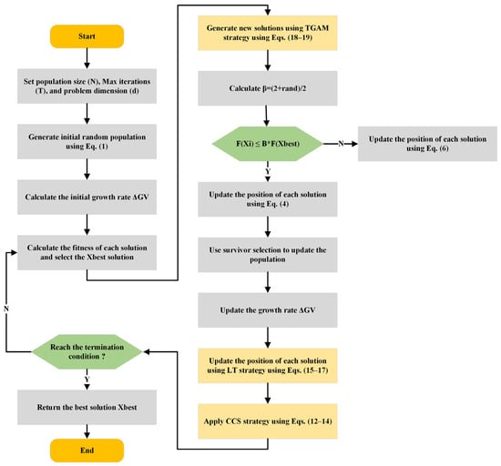
Figure 1.
The proposed ACIVY.
3.4. Computational Complexity Analysis
The computational complexity of an optimization algorithm reflects how its processing time and memory usage scale with key problem variables. For both the original IVYA and the enhanced ACIVY algorithms, complexity is determined by three primary parameters: the population size , the number of decision variables or dimensions , and the maximum number of iterations .
In the original IVYA, each solution in the population performs a position update based on either the climbing or spreading phase. These updates involve arithmetic operations across dimensions. In each iteration, fitness values are evaluated for all individuals, and the population is sorted based on fitness to maintain the best solutions. The position updates for the full population require operations per iteration. Evaluating the fitness function for each solution adds , and sorting the population introduces . However, in high-dimensional settings where is large, the dominant cost is , making the total time complexity across all iterations . The memory usage is mainly attributed to storing positions, velocities, and fitness scores for all individuals, resulting in a space complexity of .
The enhanced version, ACIVY, incorporates three additional mechanisms including CCS, LT, and TGAM to improve the balance between exploration and exploitation. These strategies introduce additional operations per iteration, but they all remain linear in the population size and dimensionality. The CCS requires arithmetic operations over selected dimensions for each solution, which scales as per iteration. The LT strategy introduces a directional update contributing a cost . The TGAM strategy introduces differential mutations resulting in cost per iteration.
Overall, the time complexity of ACIVY remains in the order of , matching that of the original IVYA. The space complexity is also , as the algorithm still stores the same set of solution vectors and associated information, with minor temporary vectors used during crossover or mutation operations that do not affect the overall memory footprint.
Finally, despite ACIVY proposing several strategic improvements to enhance the performance, it does not raise the order of computational complexity. Compared to the original IVYA, the algorithm has identical time and space scalability characteristics, but much faster convergence and more accurate solutions on a variety of optimization problems.
4. Application of the ACIVY Algorithm
4.1. ACIVY for Global Optimization
This section gives a thorough analysis of the ACIVY algorithm by describing the experimental setup, as well as examining its performance in comparison to the other optimization techniques. The analysis consists of extensive experimentation on the CEC2017 [60] and CEC2022 [61] benchmark functions, modeling various real-world optimization problems. The convergence dynamics of ACIVY, as well as the distribution of performance depicted by boxplots, are also discussed in this part. Further, comparative experiments against state-of-the-art evolutionary strategies are also provided to demonstrate the efficacy of ACIVY in handling high-dimensional and complicated optimization landscapes.
4.1.1. Experimental Configuration and Settings
Two well-known benchmark sets, CEC2017 and CEC2022, were used to test ACIVY’s optimization power. CEC2017 suite comprises 29 different functions of different characteristics- unimodal (F1 and F3), multimodal (F4–F10), hybrid (F11–F20), and composite types (F21–F30). In the meantime, CEC2022 concentrates on 12 advanced functions designed to test the performance of algorithms on deceptive as well as high-dimensional problems. Each function of both suites is defined in the domain . These testbeds are designed purposefully to test the skill of an optimizer on both exploration (global search) and exploitation (local refinement).
Moreover, the experimental run was conducted with the dimensions of 50 for CEC2017 and 20 for CEC2022. All the tests were performed with a constant population size of 30 solutions, 30,000 function evaluations, and 30 repetitions were carried out independently to make the statistical analysis meaningful. All performances were conducted on a computing system composed of a 2.60 GHz Intel Core i7 10750H CPU, 32 GB RAM, and Windows 10 (64-bit), and all codes were written in MATLAB R2020b.
For benchmarking purposes, ACIVY was assessed against a wide spectrum of MAs, categorized into three main groups. The first group includes foundational methods such as AOA [62], WOA [31], and HHO [30], all widely adopted for their general reliability. The second group contains more recently introduced optimizers like SWO [63], COA [64], CFish [65], SHO [66], GJO [67], and HMO [68], which propose recent strategies in search methodology. The third group comprises advanced and competition-winning algorithms such as eCOA [69], CMAES [39], GWO_CS [70], RDWOA [71], CSOAOA [72], DAOA [73], ISSA [74], jDE [75], and IPSO_IGSA [76], representing state-of-the-art optimization capability. Detailed settings for each algorithm are listed in Table 1.

Table 1.
Various parameter settings.
The selected benchmark algorithms to compare with are based on their proven relevance and confirmed efficiency in a wide range of optimization cases. The classical methods act as a solid background, the results of which are predictable over time, and the newer models represent the rising opinions and search strategies [77,78]. Additionally, newer and high-scoring algorithms, particularly those that have succeeded in competition, are included to ensure that the comparison framework spans a large performance range. This multi-level choice offers the opportunity to evaluate the performance of ACIVY carefully and objectively against popular, new, and state-of-the-art metaheuristics.
4.1.2. Metrics for Evaluating Optimization Performance
In order to impartially assess the quality of work of the ACIVY algorithm among these different rivals, there are a number of statistical and descriptive measures. These are the average quality of solutions (AVG), standard deviation (SD), Friedman ranking (FR), and the Wilcoxon rank-sum significant test. All the metrics have their role in the profiling of consistency, reliability, and superiority of the optimizer.
- Mean Fitness (AVG): The measure of the quality of solutions typically attained is the average fitness score over different independent runs. This measurement is useful in the evaluation of the correctness and general performance of an algorithm in repetitive usage, within the same setup. It is calculated with
- Standard Deviation (SD): SD quantifies the extent of dispersion of the fitness values around the mean, providing information about the consistency and stability of the results produced by the algorithm. Smaller variations show that the optimizer provides consistent results when repeated many times. It can be calculated as follows:
- Friedman Ranking (FR) [79]: This non-parametric statistical test ranks algorithms based on their relative performances across multiple problem instances. A lower average rank suggests a superior performance. The final ranking is derived from averaging ranks over all tested functions. The Friedman test statistic is then evaluated using a chi-squared distribution to determine consistency in relative performance across functions.
- Wilcoxon Rank-Sum Test [80]: To establish whether performance differences between ACIVY and any competing algorithm are statistically meaningful, the Wilcoxon rank-sum test is utilized. A -value below 0.05 denotes a significant difference. If ACIVY achieves better results, it is marked with ; if no clear difference exists, it is annotated with ; and if ACIVY underperforms, it is labeled with .
A combination of these metrics provides an extensive basis to compare ACIVY to other algorithms and make sure that all findings regarding the optimization performance of this algorithm are statistically aligned and indicative of its practical potential.
4.1.3. Results Discussion Using CEC2022
The main goal of this part is to compare and review the functionality of the proposed ACIVY algorithm with an extensive list of well-known optimization algorithms on the CEC2022 benchmark collection. The variety of tested algorithms embodies the various algorithmic paradigms and serves as a thorough testbed to evaluate the performance of ACIVY on a wide range of optimization problems as presented in Table 2.
Table 2.
Experimental results using CEC2022 for ACIVY and other competitors.
On the unimodal function F1, ACIVY shows an outstanding performance, having the best rank and averaged fitness of 300.367, with an extremely low standard deviation of 0.354. Such a remarkable performance implies that ACIVY converges more precisely and reliably in single-optimum landscapes. The algorithm has spectacularly beaten all competitors, with the second-best performer (HHO) having a fitness value. Such a steep rise in performance underlines how well ACIVY’s coordinated growth and adaptive mechanisms exploit unimodal search spaces. Over the multimodal functions, ACIVY shows a continuously high performance and takes the leading position on F2, F3, and F4. On F2, ACIVY attains an average fitness of 454.503, only slightly higher than the original IVY at 461.213, indicating the improvement made with ACIVY along with preserving the strengths of the core algorithm. In the case of F3, ACIVY attains the theoretical maximum of 600.000 with a standard deviation of zero, indicating absolute convergence and superb reliability. Such a huge improvement suggests that ACIVY is more capable of traversing multimodal landscapes effectively and reliably finding global optima.
Furthermore, the hybrid functions reveal ACIVY’s robust adaptability across different problem characteristics. ACIVY secures first place on F5 and F7, second place on F6, and third place on F8, maintaining an average rank of 2 across this category. Notably, on F5, ACIVY achieves a fitness value of 1402.843, substantially outperforming the second-best GJO (1891.702). The algorithm’s performance on F6 is particularly noteworthy, where it achieves the second-best result with a significantly lower standard deviation compared to many competitors, indicating superior solution stability. In the most challenging composite function category, ACIVY demonstrates consistent excellence by securing first place on F9, F10, F11, and F12. This comprehensive dominance across all composite functions is particularly significant, as these problems combine multiple optimization challenges and represent the most complex scenarios in the benchmark suite. On F9, ACIVY achieves a near-perfect performance with a fitness value of 2480.811 and an exceptionally low standard deviation of 0.054, indicating both optimal solution quality and remarkable consistency across independent runs.
The base IVY algorithm shows decent results and ends up at a rank of 4, which confirms the base idea but also shows how much better the results can be with the additions that ACIVY provides. CFish takes the second overall spot with a solid performance across many functions, and GJO completes the top three with steady mid-range rankings. Such advanced algorithms as HHO, SHO, and HMO have different performance levels, where HHO took sixth place and provided competitive results on particular functions, such as F1. Nevertheless, the performance of all these established algorithms is not consistent with the performance of ACIVY on the wide categories of functions. Moreover, the algorithms ranked last (SWO, AOA, and COA) perform especially poorly on multimodal and composite functions, and their results have a high standard deviation, which means that the algorithms do not produce reliable solutions. This comparison underlines the superiority of ACIVY in terms of robustness and flexibility on varied optimization landscapes.
The behavior of the performance of ACIVY is distinguished not only by high-quality average fitness values but also by the low standard deviations in most functions. This combination implies that ACIVY reliably converges to high-quality solutions on multiple independent runs, an important trait in the practical use of optimization. The capability of the algorithm to sustain low variance with optimal or near-optimal fitness values shows the efficiency of adaptive mechanisms and well-balanced exploration–exploitation schemes.
Having the average rank of 1.25 over all twelve functions and obtaining the last rank of 1, ACIVY confirms itself as the most efficient algorithm in this full comparative study. The large difference in performance between ACIVY and the second-placed CFish (average rank 4.00) highlights the extensive algorithmic progress that the crisscross strategy, LT strategy, and TGAM improvements bring. These findings unreservedly show that the bio-inspired improvements incorporated in ACIVY effectively overcome the weaknesses of the original IVY algorithm, without affecting its principal advantages. The outstanding performance of the algorithm in a wide variety of categories of functions confirms its applicability to real-world optimization problems, which need robust, reliable, and high-accuracy solutions.
The convergence plots show the clear optimization behavior of ACIVY on the CEC2022 benchmark functions, and it exhibits better convergence properties than the competing algorithms as shown in Figure 2. According to Figure 2, ACIVY can be characterized by fast initial convergence and subsequent stable refinement stages and is fastest in terms of fitness values in all categories of functions. The convergence curve of the algorithm can be described as having very sharp initial drop-off curves followed by very rapid stabilization at optimal or near-optimal solutions, which implies the existence of effective exploration-to-exploitation transition mechanisms within the improved ivy-inspired strategies. In the case of unimodal and simple multimodal functions (F1–F4), ACIVY shows a remarkable convergence rate and achieves optimal solutions in the initial 5000–10,000 FEs. The convergence curves depict dramatic fitness gains during the initial iterations, where F1 and F3 converged to the theoretical optimum with little variance. Conversely, the competing algorithms either converge at non-optimal solutions or have slower rates of convergence with better final fitness values. It is noteworthy that the original IVY algorithm demonstrates decent convergence behaviors but cannot compete with ACIVY in terms of accuracy and speed, which proves the efficiency of the suggested improvements.
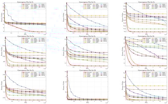
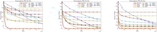
Figure 2.
Convergence curves of different algorithms using CEC2022.
The hybrid functions (F5–F8) demonstrate the strong flexibility of ACIVY to a complex landscape, with identical convergence behavior when the problem complexity is increased. The algorithm shows no or minimal oscillations and no stagnation periods associated with state-of-the-art algorithms. Function F6 and F7 especially demonstrate the high performance of ACIVY, in which the algorithm quickly converges in less than 10,000 FEs, whereas other algorithms are still struggling with either slow convergence or plateau phenomena. These functions feel the impact of the LT strategy, as they allow proper escape out of local optima, which other algorithms get stuck in. In the most difficult composite functions (F9–F12), the convergence pattern of ACIVY is extremely regular and accurate, showing the fastest descent rates and being stable during the optimization process. F11 and F12 demonstrate the capability of the algorithm in finding optimal solutions in these complex multimodal landscapes, whereas ACIVY either gets stuck in local optima or exhibits unstable convergence behavior. The attribution of the TGAM strategy is especially reflected in these functions, which allow an easy transition between exploration and exploitation stages without affecting the quality of the convergence. Such a high convergence performance in all types of functions proves the efficiency of ACIVY as a strong and trustworthy optimization algorithm to handle complex real-world problems.
On the other hand, the boxplot analysis shown in Figure 3 thoroughly reveals the statistical distribution nature and the reliability of the solution of ACIVY versus the rival algorithms on the CEC2022 benchmark functions. The boxplots display important performance metrics such as median fitness values, quartile ranges, the existence of outliers, and the overall consistency of solutions. ACIVY achieves statistical excellence in all aspects regarding medians, interquartile ranges, and the presence of outliers, showing the quality of the solution is optimal and the algorithm is very stable across all types of functions.
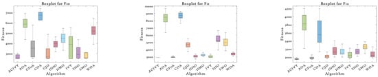
Figure 3.
Boxplots of different algorithms using CEC2022.
In the case of unimodal and multimodal functions (F1–F4), ACIVY shows the tightest boxplot distributions with the lowest median fitness values and minimal interquartile ranges. On F1, the boxplot of ACIVY is incredibly tight and centered around the theoretical optimum, whereas the competitors have much broader ranges and larger medians. The F3 boxplot especially shows the superiority of ACIVY, which has reached perfect convergence with zero variance, displayed as a single horizontal line at the optimal value of 600. Conversely, other algorithms, such as AOA and COA, exhibit very long whiskers and several outliers, which reflect the lack of consistency and reliability of the solution. The hybrid functions (F5–F8) illustrate the strong stability performance of ACIVY with regard to its boxplot structures that tend to be small even in multi-dimensional optimization landscapes. F6 shows that ACIVY has an outstanding performance with a very narrow distribution and low median, whereas competitors have large ranges and many outliers. The effect is especially dramatic when the compact boxplot of ACIVY is compared with the extremely wide distribution of COA spanning several orders of magnitude. F7 and F8 additionally affirm the statistical superiority of ACIVY, with low variance and ideal median rankings in comparison to the random and unreliable distributions of the rival algorithms. The composite functions (F9–F12) demonstrate the ultimate statistical excellence of ACIVY with the best median performance and superior distribution tightness. ACIVY ensures the minimum median values of all composite functions and shows an impressive consistency expressed in small boxplot ranges. This superiority is illustrated on F11, where ACIVY obtains a compact distribution with short whiskers, whereas the other algorithms, such as AOA and COA, exhibit a large population of outliers and broad quartile sticks. The statistical experiment appears to clearly indicate that ACIVY is not only capable of higher optimization performance but also offers the best degree of algorithm robustness and predictability which are critical properties of algorithms intended to be used in practice and needed to generate high-quality solutions consistently.
The testing of statistical significance is an important aspect in the optimization algorithm performance superiority proofs, as the observed performance gains can be easily attributed to random fluctuations [81]. The analysis of MAs must be accompanied by sound statistical testing in order to determine the confidence of comparative outcomes, especially in the case of stochastic optimization algorithms, which are by nature prone to variation with multiple independent runs. In this analysis, two basic non-parametric statistical tests are used: the Friedman test to evaluate the overall ranking and the Wilcoxon rank-sum test to compare each pair of algorithms, respectively, which were explicitly invented to work with non-normal distribution data, as optimization algorithm performance data often is.
Figure 4 shows the results of the Friedman test, which gives a full ranking analysis of each of the algorithms on the entire CEC2022 benchmark suite. ACIVY attains the best average rank of 1.66 and significantly outcompetes all the competing algorithms and statistically dominates them in varying optimization landscapes. The original IVY algorithm still achieves a respectable average rank of 4.92, confirming the validity of the underlying approach but pointing to the immense gains made by ACIVY’s enhancements. The ranking order shows the existence of specific performance levels, where CFish (4.29) and GJO (4.61) comprise the second performance level and HHO (4.79) and SHO (5.00) belong to the middle-level performances. HMO (5.97), SWO (7.74), and WOA (7.76) are placed in the bottom part of the ranking, and AOA (9.58) and COA (9.68) take the last places. Such statistical ranking proves the outstanding ability of consistency in the performance of ACIVY in all categories of functions, and this shows its great flexibility in facing different kinds of optimization problems.
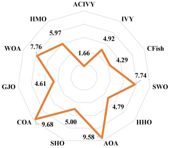
Figure 4.
Friedman ranks various algorithms using CEC2022.
On the other hand, Figure 5 shows the pairwise Wilcoxon rank-sum test results, which extensively statistically prove the superiority of ACIVY over each of the competing algorithms in a pairwise manner. The analysis shows the clear statistical overpowering of ACIVY with higher performance () values varying between 10 and 12 functions over all the competitors, whereas the values are always zero in all of the pairwise comparisons. Compared to AOA, CFish, COA, GJO, HHO, HMO, SWO, and WOA, ACIVY has statistical dominance (shows a better performance on 12 functions and never performs worse on any of the 12 functions). ACIVY also performs better on 10 functions against IVY and SHO, with 2 ties (), and once more, 0 worse performances. The values suggest that there are some statistical ties with CFish and GJO (one function each) and SHO (two functions), but these are not losses but statistical ties, which once again underline the superiority of ACIVY across the board.
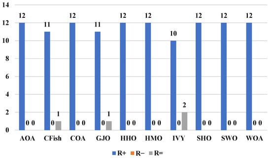
Figure 5.
Wilcoxon test results for ACIVY versus other algorithms using CEC2022.
This statistical evidence gives unquestioning confirmation of the algorithmic superiority of ACIVY over the benchmark suite. The Friedman test confirms the superior position of ACIVY with the minimal average rank of 1.66, and the Wilcoxon rank-sum test proves the overall superiority of the former with its pairwise wins. Overall, the lack of values (zero inferior performances) in all algorithmic comparisons is a startling statistical feat, which means that ACIVY does not show a worse performance than any of its competitors on any of the benchmark functions. This stable trend of statistical significance, together with the large performance gaps demonstrated by the Friedman ranks, gives strong indications that the improvements found by ACIVY are not fluctuations but actual algorithmic advances. The statistical strength of these findings puts high confidence in the reliability and efficacy of ACIVY, making it a statistically proven method of handling complex optimization problems where not only is excellent performance needed, but also reliability across a wide range of problem landscapes.
4.1.4. Results Discussion with Advanced Algorithms Using CEC2017
In this section, the performance of ACIVY is compared with state-of-the-art algorithms on the CEC2017 benchmark suite of 50-dimensional problems, which, together with the earlier analysis on CEC2022, gives a thorough verification of the algorithm on various benchmark standards and problem dimensions. The comparative analysis involves ten advanced algorithms, namely, eCOA, CMAES, DAOA, CSOAOA, GWO_CS, RDWOA, jDE, ISSA, and IPSO_IGSA, which are recent advancements in evolutionary computation, swarm intelligence, and hybrid optimization techniques.
According to Table A1, ACIVY shows a remarkable performance advantage throughout the CEC2017 benchmark set, taking the final overall first rank with an incredible average rank of 1.41, which is significantly better than all other participating advanced algorithms. The algorithm ranks first on 20 of 29 functions (win rate of 69.0%), ranks second on 7 functions, third on F17, and fourth on F10, giving a top-two result on 93.1 percent of the benchmark problems. CSOAOA turns out to be the second-best-performing with the final rank of second (average rank 3.17), and GWO_CS ranks third (average rank 3.72), and eCOA ranks fourth (average rank 3.79). The performance hierarchy shows that there are large differences between ACIVY and its nearest rivals, where DAOA is placed at the bottom (final rank 10, average rank 10.00), indicating the existence of large algorithmic advantages of ACIVY. Function category analysis reveals ACIVY’s performance patterns across diverse optimization landscapes with distinct characteristics for each problem type. For unimodal functions (F1, F3), ACIVY achieves perfect dominance with a 100% win rate (two out of two functions), demonstrating exceptional exploitation capabilities where F1 shows a fitness value of 6296.553 compared to DAOA’s 2.83 × 10¹¹. In multimodal functions (F4–F10), ACIVY secures first place on only two functions (F4 and F6), achieving a 28.6% win rate, but maintains a strong performance with second place on F5, F7, F8, and F9, and fourth place on F10. Despite the lower win rate, ACIVY’s fitness values remain highly competitive, with F4 showing 506.774 versus competitors ranging from 643.383 to 1.04 × 10⁵. The hybrid functions category (F11–F20) showcases ACIVY’s superior adaptability with an 80% win rate (8 out of 10), securing first place on F11, F12, F13, F14, F15, F16, and F18, with second-place finishes on F19 and third place on F17. In this category, F12 particularly exemplifies ACIVY’s dominance with a fitness value of 5.89 × 10⁶ versus DAOA’s 1.41 × 10¹¹. For composite functions (F21–F30), ACIVY demonstrates remarkable consistency with 80% superiority (8 out of 10), winning on F20, F21, F23, F24, F25, F26, F27, F28, and F29, while achieving second place on F30 and F22. The performance distribution reveals ACIVY’s exceptional strength in complex hybrid and composite functions, where its enhanced mechanisms prove most effective.
The comparative analysis reveals significant fitness value disparities between ACIVY and advanced competitors across critical benchmark functions. On function F1, while ACIVY achieves 6296.553, its closest competitor, ISSA, reaches 1.76 × 10⁸, representing a large performance gap, with other algorithms like CMAES and DAOA performing orders of magnitude worse. Function F12 demonstrates even more dramatic differences, where ACIVY’s 5.89 × 10⁶ substantially outperforms eCOA’s 3.83 × 10⁸ and completely dominates DAOA’s catastrophic 1.41 × 10¹¹. In the hybrid function F14, ACIVY maintains 1.78 × 10⁵ while advanced algorithms like CMAES struggle with 2.14 × 10⁷, and DAOA fails at 3.46 × 10⁸. These substantial performance margins highlight ACIVY’s superior convergence precision and global search capabilities compared to even the most sophisticated contemporary algorithms. Furthermore, ACIVY consistently achieves lower standard deviation values, indicating superior solution reliability compared to competitors that often exhibit high variance and inconsistent performance across independent runs.
The Friedman test statistical significance of the CEC2017 benchmark shown in Figure 6 generates the statistical dominance of ACIVY with a mean rank of 1.78, which is significantly better than all the sophisticated competitors on the 50-dimensional optimization search space. CSOAOA proves to be the most competitive algorithm with a mean rank of 3.21, slightly followed by eCOA 3.92, meaning that these algorithms are moderately competitive, irrespective of the fact that their performances differ significantly. There are the middle-tier GWO_CS (4.17) and ISSA (4.49), and the weak overall performance of such algorithms as CMAES (5.91), RDWOA (6.38), and IPSO_IGSA (7.01). The low-ranking algorithms, jDE (8.57) and DAOA (9.55), exhibit notably bad adaptation to high-dimensional optimization problems, where DAOA is ranked among the last in the majority of the functions.

Figure 6.
Friedman ranks different advanced algorithms using CEC2017, 50D.
On the other hand, the Wilcoxon rank-sum test results shown in Figure 7 provide comprehensive pairwise validation of ACIVY’s dominance, revealing overwhelming statistical superiority against all competing algorithms. ACIVY demonstrates complete dominance against CSOAOA, DAOA, GWO_CS, ISSA, RDWOA, eCOA, and jDE with R+ values of 20, 29, 22, 29, 25, 29, 24, and 29, respectively, while maintaining zero values across all comparisons. Against CMAES, ACIVY shows superior performance on 21 functions with only 3 inferior performances and 5 ties, representing a 7:1 win-to-loss ratio. The values indicate occasional statistical ties with CMAES (5), CSOAOA (9), GWO_CS (7), RDWOA (4), and jDE (5), but these represent performance equivalence rather than losses. The absence of values against most algorithms demonstrates ACIVY’s remarkable consistency in outperforming advanced state-of-the-art methods across diverse optimization scenarios, establishing unequivocal statistical evidence of its algorithmic superiority in high-dimensional optimization contexts.
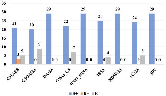
Figure 7.
Wilcoxon test results of ACIVY versus other advanced algorithms using CEC2017.
4.2. ACIVY for Engineering Problems
To assess the real-world effectiveness of the proposed ACIVY algorithm, it is applied to a suite of well-known engineering design problems. These include optimization tasks such as the design of a welded beam, speed reducer problem, tension/compression spring, tubular column, robotic gripper, speed reducer, and three-bar truss design problem. Each problem includes a set of design constraints, which are handled using a static penalty mechanism as outlined in Equation (22) [82].
In this penalty-based formulation, the modified objective function is expressed as , where is the original objective. The penalties are incorporated using the terms and , which are positive constants. The expressions and correspond to inequality and equality constraints, respectively. To control the severity of penalties, exponents and are introduced, each set to either 1 or 2, depending on the constraint handling requirements.
Each engineering problem is solved under identical algorithmic settings to ensure fair performance comparison. The experimental setup includes a fixed population size of 50, a total of 500 iterations, and 30 separate runs for each problem to obtain statistically meaningful results. The main mathematical modelling of these problems is presented in Appendix A.
4.2.1. The Tension–Compression Spring Design Problem
The tension–compression spring design (TCSD) task can be described as follows [83]: given the total weight of the spring, find the minimum possible weight subject to a number of engineering-based constraints. The proposed optimization problem can be characterized by three primary variables, including the thickness of the wires , the mean diameter of the coils , and the number of active coils . These variables need to be finely tuned to meet design specifications regarding stresses limits, deformation limits, and mechanical reliability. The resulting design should be able to resist tension and compression forces, the material must be used efficiently, and the spring life should be maximized. It is used as a benchmark to evaluate the effectiveness and constraint-handling capability of state-of-the-art metaheuristic algorithms. The mathematical model of this problem can be found in Appendix A. Table 3 shows the results of running the performance evaluation assignment uses the tension–compression spring design problem to illustrate that ACIVY has an outstanding optimization ability. ACIVY provides the best mean fitness value of 0.012665233 with an extremely small standard deviation of 8.69008 × 10⁻¹⁷, which implies flawless convergence uniformity throughout the 30 independent runs. This performance is impressively better than all the competing algorithms, with the nearest rival TTAO having a mean fitness of 0.012705868 and a much larger standard deviation of 2.27993 × 10⁻⁵. The good performance of the algorithm is also revealed by the fact that it found the same best and worst fitness, which has never been seen before in terms of reliability and robustness in handling constraints and global optimization. The optimal design parameters obtained by ACIVY and other comparative algorithms, as shown in Table 4, reveal a well-balanced engineering solution with a wire diameter () of 0.0516890607, a mean coil diameter () of 0.356717730, and a number of active coils () of 11.2889664, resulting in the best fitness value of 0.0126652328. Compared to other algorithms, ACIVY’s parameter configuration represents a practical and manufacturable design that effectively balances material usage with structural performance requirements.
Table 3.
Statistical results for different algorithms on the tension–compression spring problem.
Table 4.
The obtained parameters of the tension–compression spring problem.
4.2.2. Weight Minimization of a Speed Reducer
The speed reducer design problem represents a well-known case in mechanical engineering optimization, where the primary goal is to minimize the total mass of a gearbox assembly without compromising its mechanical performance or its compatibility with connected components such as the engine and propeller system [23]. Reducing the system’s weight not only improves energy efficiency but also contributes to better operational performance and reduced load on supporting structures. The seven design variables that correspond to this problem represent an important geometry or mechanical behavior feature of the reducer. The optimization algorithm is subject to numerous design constraints, which include material strength, stress tolerances, and geometric feasibility. The mathematical model of this problem can be found in Appendix A. The optimization results for the speed reducer design problem, presented in Table 5, demonstrate ACIVY’s exceptional performance in handling complex multi-dimensional constrained optimization. ACIVY achieves an optimal mean fitness value of 2713.031561 with an extraordinarily small standard deviation of 0.000149, indicating remarkable consistency and reliability across all independent runs. This performance significantly surpasses competing algorithms, with the second-best performer, TTAO, achieving a nearly identical mean fitness of 2713.034866 but with a substantially higher standard deviation of 0.009914. The algorithm’s superiority is further emphasized when compared to other methods like SWO (2845.973890) and SCA (2857.789669), which show a considerably worse performance with high variance, demonstrating ACIVY’s robust capability in navigating the complex constraint landscape of this seven-dimensional optimization problem.
Table 5.
Statistical results for different algorithms on the speed reducer engineering problem.
Moreover, the optimal design parameters obtained by ACIVY, as detailed in Table 6, reveal a well-engineered solution with a face width () of 2.80700516, module of teeth () of 0.70000000, number of teeth on pinion () of 17.00000000, shaft lengths () of 7.30000000 each, and bearing diameters () of 3.35054095 and 5.28651792, respectively, resulting in the best fitness value of 2713.03156062. Notably, ACIVY and MFO achieve close parameter configurations, indicating convergence to the true global optimum, while other algorithms like SWO and WOA show significant deviations from optimal values, particularly in the variables , , and . The parameter analysis reveals that ACIVY consistently identifies design configurations that satisfy all mechanical constraints while minimizing weight, with several variables converging to boundary values (), suggesting these represent critical design limits for optimal performance in speed reducer applications.
Table 6.
The obtained parameters of the speed reducer engineering problem.
4.2.3. Welded Beam Design Problem
This optimization problem addresses the cost-effective manufacturing of a welded beam structure [84]. The objective is to minimize the fabrication cost by adjusting four geometric parameters: weld thickness , beam height , beam length , and beam flange thickness . The mathematical model of this problem can be found in Appendix A. The optimization results for the welded beam design problem, presented in Table 7, showcase ACIVY’s outstanding performance in minimizing fabrication costs while satisfying complex structural constraints. ACIVY achieves an optimal mean fitness value of 1.67021773 with an exceptionally small standard deviation of 0.00000006, demonstrating near-perfect convergence consistency across all runs. This performance substantially outperforms the competing algorithms, with TTAO achieving a very close mean fitness of 1.67021777 but with a significantly higher standard deviation of 0.00485478. The algorithm’s superiority becomes more pronounced when compared to other methods such as SWO (3.13525785), TSA (2.09364637), and WOA (2.41742026), which exhibit a considerably worse performance with high variance, indicating ACIVY’s exceptional capability in handling the nonlinear constraints and complex design space of this structural optimization problem.
Table 7.
Statistical results for different algorithms on the welded beam engineering problem.
The optimal design parameters obtained by ACIVY, as detailed in Table 8, reveal a highly efficient structural configuration with a weld thickness () of 0.1988323072, beam height () of 3.3373652986, beam length () of 9.1920243225, and beam flange thickness () of 0.1988323072, resulting in the best fitness value of 1.67021772. The parameter analysis shows that ACIVY, TTAO, and several other algorithms converge to close values, confirming the global optimum identification. Notably, ACIVY achieves perfect symmetry with , indicating an optimal design balance between weld and flange thicknesses. In contrast, algorithms like SWO and TSA show significant parameter deviations, particularly in the beam height () values of 5.3649639962 and 3.4191767660, respectively, resulting in substantially higher costs and demonstrating ACIVY’s superior constraint handling and convergence precision in structural design optimization applications.
Table 8.
The obtained parameters of the welded beam engineering problem.
4.2.4. Three-Bar Truss Design Problem
This design optimization scenario focuses on a traditional three-bar truss structure exposed to applied external forces [85]. The primary aim is to reduce the overall use of material—quantified by the structure’s weight—while guaranteeing that stress levels across all members remain within permissible limits when subjected to loading. The decision variables in this model are and , representing the cross-sectional areas of the horizontal and angled (diagonal) elements of the truss, respectively. The mathematical model of this problem can be found in Appendix A. The optimization outcomes of the three-bar truss design problem in Table 9 show that ACIVY is very effective in minimizing the weight of the structure subject to the satisfaction of stress constraints. ACIVY provides a higher mean fitness value of 98.9054388 with an incredibly small standard deviation of 0.0000002, which implies excellent consistency and stability throughout the optimization runs. This compares favorably to most of the competing algorithms with a few having a slightly higher mean fitness value of 98.9675309 but almost a similar standard deviation of 0.0000003. The advantage of using the algorithm can be observed compared to approaches such as SWO (98.5799219 +/− 2.5137111) and SCA (99.7838562 +/− 1.5109708), which showed much higher variance and less guaranteed convergence, showing the strong performance of ACIVY in searching the nonlinear constraint space of this structural optimization problem.
Table 9.
Statistical results for different algorithms on the three-bar truss engineering problem.
The design parameters yielded by ACIVY, tabulated in Table 10, indicate the optimum design with the structure showing an efficient configuration with cross-sectional areas = 0.270343428 and = 0.225028620, having the best fitness value of 98.905430382. Interestingly, ACIVY, DOA, and IVY appear to converge to the same parameter values of both design variables, indicating convergence to the actual global optimum region. The parameter analysis indicates that the ACIVY has the best performance in terms of the cross-sectional area of the horizontal member () and diagonal member (), where the horizontal member needs around 20% more cross-sectional area to accommodate the structural loads efficiently.
Table 10.
The obtained parameters of the three-bar truss engineering problem.
4.3. ACIVY for UAV Path Planning Optimization
In order to evaluate the practical relevance of the suggested ACIVY algorithm, its performance is considered in the area of unmanned aerial vehicle (UAV) navigation planning. Based on the fundamental assessments presented in Section 4.1 and Section 4.2, in which ACIVY demonstrated stable superiority over traditional and state-of-the-art MAs on the CEC2017 and CEC2022 benchmarks, this section applies it to the UAV path planning problem. The benchmark functions are renowned for having complicated traits such as high dimensionality, nonlinearity, and discontinuities that serve as good analogues of the problems posed by UAV trajectory design. Accordingly, the ACIVY algorithm will be tested in a simulated setting with circular areas of threats, as seen in real-life applications in defense, surveillance, and autonomous aerospace missions.
The UAV path planning problem can be formulated as follows: given a certain starting point and destination, find a trajectory that is optimal in some sense, with the constraints of operating in an environment filled with potential obstacles and operational constraints [86]. Such risks might be in the form of terrain obstacles, enemy detection areas, or restricted airspaces. Moreover, the UAV has to observe physical limitations such as fuel capacity, dynamics, and maneuverability limits, like the turn radius and maximum climb rate. The operating environment is often idealized to a 2D or 3D grid with geometric obstacles, frequently assumed to be circles or polygons.
In this configuration, the object has to drive around doughnut-shaped areas, which are interpreted as regions of high risk, e.g., radar detection fields or dangerous terrain. Figure 8 depicts that the UAV is initially at a known starting point and has to reach the desired destination . The direct line between and is split into segments equally, which brings flexibility to the routing procedure. Also, the lines , ,…, , perpendicular to the segmentation points are constructed. The lines each delineate a plane of potential discrete waypoints amongst which one optimum point may be chosen.
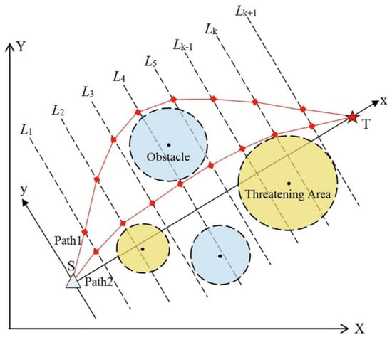
Figure 8.
UAV path planning diagram [86].
By connecting one point on each of these perpendicular segments in consecutive fashion, a closed and valid flight path is created that meets mission requirements and avoids any prescribed threat areas or restricted areas. Using this structure, a flexible, but constrained, optimization problem is enabled to precisely capture the nature of the operational needs of autonomous UAV systems. The complete set of navigation points is rigorously stated as
Such a discrete representation enables the ACIVY algorithm to search through a wide range of feasible paths and converge to one that achieves the minimization of exposure and fuel consumption and the feasibility of the route, considering environmental and vehicle-specific constraints. A coordinate transformation is used to ease the calculations and to match the optimization direction with the geometry of the problem. The transformation that moves the segment into the new x-axis is
where
Here, represents the angular deviation between the original x-axis and the segment , allowing the trajectory generation to occur along a normalized reference frame. The fitness function used in this case is defined in terms of cost and fuel as shown in Appendix A.
To thoroughly evaluate the proposed ACIVY algorithm in the context of UAV navigation, simulation experiments are carried out across different environmental configurations, each populated with circular threat zones. These test cases differ in threat zone density, spatial positioning, and risk magnitude, simulating a wide range of practical mission scenarios. The UAV begins its flight at position (2,2) and is required to reach the target location at (3299,3299), modeling a long-distance mission through potentially adversarial or restricted airspace.
The experimental configuration is the same in all the simulations. We limit each optimization process to 1000 iterations, and the size of the population is 30 solutions per generation. The problem space is characterized by 10 dimensions, which is equal to the number of intermediate decisions that constitute the path of the UAV. Each algorithm is run independently 30 times to make the statistical results reliable and consider the stochasticity of MA. The result of each run is stored, and such key performance indicators as the best, worst, average, and standard deviation of the final cost are calculated to compare.
The performance of ACIVY is compared to some well-known metaheuristic algorithms, which are the original Butterfly Optimization Algorithm (BOA) [87], Crayfish Optimization Algorithm (CFish) [65], Human Memory Optimization (HMO) [68], Tunicate Swam Algorithm (TSA) [88], Arithmetic Optimization Algorithm (AOA) [62], Coati Optimization Algorithm (COA) [64], and the original IVYA algorithm. The mentioned algorithms are well known to be successful in solving continuous and constrained optimization problems with nonlinear objective functions.
The strength and correctness of ACIVY are approved in three test cases that represent various spatial distributions of circular threat zones. The scenarios, as concluded in Table 11, differ in the concentration of obstacles, size, and intensity, providing a wide range of assessments. These findings demonstrate that ACIVY is not only an efficient method to deal with nonlinear and high-dimensional trajectory optimization but also it is stable in various runs.
Table 11.
Description of threats in the 3 cases.
As observed in Table 12, the results of the performance evaluation of Case 1 show that ACIVY is exceptionally competent in resolving the UAV path planning optimization problem in the first threat scenario setup. ACIVY provides the best performance in terms of all the statistical metrics because it has the best fitness value of 2502.12372, a mean fitness of 2502.32598, and the standard deviation is extremely low, 0.264660329. This extreme performance is properly several times faster than any of the competing algorithms, with the nearest rival BOA having a best fitness of 2504.41698 and a mean of 2506.60476, making the performance difference between this and the other algorithms. The advantage of the algorithm performance is even more significant in comparison to such methods as CFish (mean: 2536.58402 +/− 27.02260666) and TSA (mean: 2532.1528 +/− 16.26598301) that have a significantly higher cost and variance.
Table 12.
Statistical metrics for Case 1.
The statistical comparison shows a remarkable consistency and reliability of ACIVY in UAV mission planning, as its standard deviation is extremely low compared to all the competitors. Though such algorithms as IVY (2508.98792 +/− 2.318207734) and HMO (2510.85416 +/− 2.372573147) demonstrate a certain consistency in performance, they remain far behind in accuracy when compared to ACIVY. Such consistency is especially important in real-world UAVs where the reliability of missions and predictability of performance are top priorities, and as seen in the case of ACIVY with a relatively small gap between the best (2502.12372) and worst (2502.8327) performance values, shows the robustness of its algorithm in dynamic path planning tasks.
The visual optimal paths computed by each algorithm in Case 1, presented in Figure 9, show the different high-level strategies of threat avoidance and trajectory optimization. The trajectory of ACIVY shows better spatial intelligence, as it follows the best balance between directness and safety, performing smooth curved movements to optimally go around the six circular threat areas while keeping the distance and the threat levels minimal. The trajectory covered by the algorithm has a well-chosen waypoint that results in smooth arcs around the high-risk regions, especially visible in how it avoids the large threat area in the center and the concentration of threats in the upper-right quarter. Conversely, other algorithms, such as TSA and COA, are more conservative and exhibit extreme curvature that leads to higher fuel consumption, whereas BOA and HMO tend to produce angles that are too sharp and could lead to UAV maneuverability limitations.
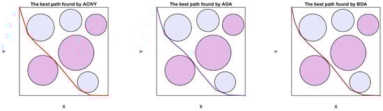

Figure 9.
Path planning results for Case 1 using various algorithms.
The comparative analysis shows a wide disparity in the quality and feasibility of paths found by the competing algorithms. The path of ACIVY shows a constant clearance margin to all threat boundaries without sacrificing the smoothness of the flight path, which implies a better constraint handling and multi-objective optimization ability. The algorithm is able to find the optimal corridor along the complex threat landscape without making unnecessary detours, and without entering dangerously close to high-intensity threat areas. Other algorithms, such as CFish and GKSO, exhibit a poor path planning performance, either by going too near the high-risk regions or by making unnecessary long diversions, which leads to an increase in the cost of the mission.
The convergence curve of Case 1, shown in Figure 10, indicates the outstanding optimization dynamics and the excellent convergence properties of ACIVY within the UAV path planning application field. ACIVY shows the most aggressive and effective early-stage convergence behavior, falling quickly out of an initial cost of about 2900 to near-optimal costs of about 2500 in the first 100 iterations. Such a fast convergence implies that the algorithm has strong exploration abilities and effective search space exploration, which makes it quick to find and exploit good areas of the solution space. The algorithm shows consistent progress in optimization, and in the end, gives the minimum final cost compared to any other competitor. Comparatively, the GKSO and BOA algorithms exhibit slower rates of initial convergence, whereas CFish and TSA exhibit less reliable improvement trends with temporary periodical stagnation.
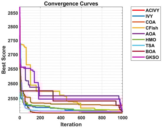
Figure 10.
Convergence curve for Case 1.
The convergence stability plot indicates the excellent consistency and stable optimization pattern of ACIVY during the 1000 iterations. Following the fast initial progress, ACIVY continues with a smooth and steady refinement process, which is evidence of well-balanced exploration and exploitation dynamics that avoid premature convergence, at the same time guaranteeing a constantly improving solution. The convergence curve of the algorithm has very few variations with no observable plateaus, indicating strong local optima escape mechanisms and good global search abilities. Such consistent convergence behavior is in stark contrast to other algorithms, such as COA and HMO, that show erratic convergence behavior with many plateau periods and little progress in later iterations. The enviable convergence traits of ACIVY are in direct proportion to its statistical performance indices, thus validating the role played by the increased bio-inspired strategies in the algorithm to convert the high convergence rate into a steady state of optimal solution quality in the testing UAV path planning environments.
Case 2 performance analysis presented in Table 13 shows that ACIVY remains a clear leader in dealing with more complex threats, with the best fitness value of 2374.11064 and an incredible consistency demonstrated by the standard deviation of just 0.234912478. This constitutes a strong performance improvement over its nearest rival, BOA, which has a best fitness of 2375.47342 and a mean of 2376.87129, showing that ACIVY optimizes better in this harder threat landscape. The performance of the algorithm is further accentuated when compared to algorithms suffering significantly during the higher threat density, especially CFish (mean: 2470.77789 +/− 65.84699354) and TSA (mean: 2451.45497 +/− 32.77127957), which demonstrate extreme performance degradation and high variance in the Case 2 complex scenario.
Table 13.
Statistical metrics for Case 2.
On the other hand, Figure 11 shows the visualization of Case 2, which indicates that ACIVY outperformed its spatial reasoning skills in the more challenging threat landscape consisting of eight distributed circular areas with different intensities. The trajectory of ACIVY is characterized by remarkable strategic analysis, showing the best path across the thick threat field, keeping an almost straight line, but carefully bypassing all high-risk sectors. The track of the algorithm illustrates highly advanced waypoint selection to develop a smooth executable path with minimal offset to the straight-line distance, efficiently balancing the two competing goals of threat avoidance and fuel optimization. It is worth noting that the ACIVY route includes going between the central large threats with safe clearance margins, demonstrating the high level of constraint processing in the complex multi-threat case.
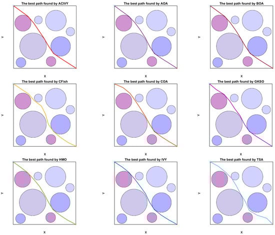
Figure 11.
Path planning results for Case 2 using various algorithms.
The comparison demonstrates that the difference in the quality of paths found by the competing algorithms vastly widens in the presence of greater environmental complexity. TSA shows the most cautious case of over-curvature that significantly adds mission distance and fuel burn, and CFish displays improper planning of an unjustifiably winding track that generates numerous direction alterations. Other algorithms, such as AOA, BOA, and COA, perform moderately well on relatively straight-line paths but do not have the accuracy of the best corridor discovery exhibited by ACIVY.
The convergence pattern in Figure 12 shows that ACIVY in Case 2 is adjusted remarkably well to higher complexity in the environment, and the optimization dynamics were faster than in Case 1. ACIVY also converges to near-optimal values of around 2380 after only 50 iterations, demonstrating that it explores the more crowded threat environment of Case 2 more efficiently. The algorithm retains its typical smooth convergence profile with no oscillations or early stagnation and ends up with the final minimum cost among all the competitors. This improved convergence rate in Case 2 indicates that the improved strategies in ACIVY are specifically suitable for the complex multi-threat environment where the traditional algorithms fail due to higher computational requirements and the complexity of the solution space.
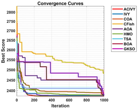
Figure 12.
Convergence curve for Case 2.
Finally, the Case 3 performance evaluation at Table 14 shows a much complex optimization terrain with ten threat zones, but ACIVY stays on the leadership track with the best fitness value of 2433.65864, indicating a high-quality solution even in the complex environment. Nevertheless, Case 3 demonstrates some curious performance patterns according to which the standard deviation (24.2325059) in ACIVY is higher than in the former cases, which might be interpreted as the increased complexity of the given threat constellation. Our nearest rival, COA, shows a competitive average performance of 2444.96932 with very low variance (4.0979329), whereas IVY is consistently ranked second with a best fitness of 2441.37365 and acceptable reliability (16.9353954 standard deviation). The performance of such algorithms as CFish (2478.17905 +/− 6.22824561) and AOA (2478.61011 +/− 9.35102086) is worse than in previous instances, which proves the higher level of optimization challenge provided by the dense threat configuration of Case 3.
Table 14.
Statistical metrics for Case 3.
Statistical analysis yields the peculiar challenge profile of Case 3, in which the ten-threat setting provides a more intricate optimization terrain and challenges the robustness and adaptiveness of the algorithms. Although ACIVY achieves the optimal individual solution, the higher variance implies that this specific threat configuration contains local optima issues, which sometimes impact the consistency of convergence. In this case, COA shows an excellent stability with the least standard deviation compared to other algorithms, which means that it is able to handle constraints well, even though it finds suboptimal solutions. The difference between the best (2433.65864) and mean (2444.2745) performance of ACIVY demonstrates that though the algorithm can find optimal corridors in the maze of threatening agents, convergence to the global optimum becomes more difficult in this crowded environment, which shows the implied complexity of ten-threat navigation scenarios with regards to UAV path planning problems.
Figure 13 presents the path routes for various algorithms in Case 3, which indicates the tremendous complexity caused by the ten-threat array, with ACIVY displaying highly advanced spatial navigation through the densest threat array in the experiment. The path of ACIVY demonstrates a high-level optimization of waypoints, as it found a viable corridor that demands careful maneuvering around several tightly spaced threats, especially in its lower part, where the algorithm has to thread the needle between the close group of four threats, still keeping safe clearance distances. The route exhibits a degree of tactical flexibility in that the curvature is controlled and varies dynamically according to the threat proximity, giving a smooth but dynamic route that balances the needs of directness with the safety constraints. Such an advanced navigation feature is the main difference between ACIVY and its competitors, TSA and IVY, which are characterized by less aggressive styles but with too many deviations that prolong the mission time and fuel usage.
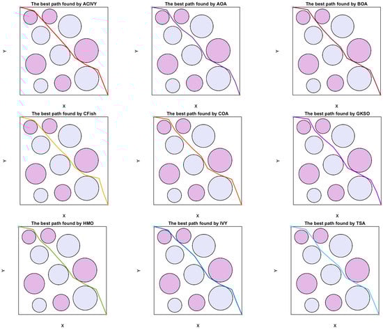
Figure 13.
Path planning results for Case 3 using various algorithms.
Moreover, to address the challenge of real-world applicability and demonstrate the robustness of ACIVY in handling complex geometric configurations beyond simple circular obstacles, an additional experimental scenario was designed involving 3D path planning through an oil plant industrial environment [89,90]. This complex scenario represents a significant advancement from the previous circular threat zone experiments, incorporating realistic industrial structures, including pipelines, storage tanks, processing units, and multi-level platforms that UAVs commonly encounter in industrial inspection and monitoring missions. The oil plant environment presents a particularly challenging navigation landscape due to its intricate 3D geometry, varying obstacle heights, narrow corridors between equipment, and the critical safety requirements inherent in petrochemical facilities where collision avoidance is paramount.
The statistical performance analysis presented in Table 15 demonstrates ACIVY’s exceptional capability in navigating this complex 3D industrial environment, achieving the best fitness value of 31.97736 with a remarkably low standard deviation of 0.11129, indicating superior consistency and reliability across multiple optimization runs. ACIVY’s performance is closely matched by BOA, which achieves an identical best fitness of 31.97736 but with higher variance (0.36918), while HMO ranks third with a competitive performance (32.07374 ± 0.25926). The algorithm significantly outperforms other competitors, with IVY showing a substantially degraded performance (44.39475 ± 4.76428) and CFish struggling considerably in this complex environment (46.96253 ± 1.43415). The visual path planning results illustrated in Figure 14 clearly demonstrate the superior spatial reasoning capabilities of ACIVY, which successfully identifies optimal corridors through the dense industrial infrastructure while maintaining safe clearance margins from all structural components. The trajectory generated by ACIVY exhibits remarkable smoothness and directness, efficiently navigating between multi-level structures and avoiding collision with complex geometric shapes, including cylindrical tanks, rectangular processing units, and interconnected piping systems. In contrast to the smooth, efficient trajectory generated by ACIVY, competing algorithms exhibit various degrees of suboptimal behavior, including unnecessary detours, inefficient altitude changes, and potentially hazardous proximity to industrial equipment. The path visualization reveals that while some algorithms like BOA and HMO produce relatively acceptable routes, others, such as CFish and IVY generate highly irregular trajectories with excessive maneuvering that would be impractical for real UAV operations, thereby validating the enhanced optimization strategies integrated into ACIVY for handling real-world complex geometric constraints in critical industrial applications.
Table 15.
Statistical metrics for complex 3D path planning.
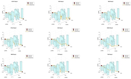
Figure 14.
Map of shortest obtained path of 3D oil plant’s path planning.
4.4. Results Discussion
The comprehensive experimental validation demonstrates ACIVY’s consistent superiority across diverse optimization domains. ACIVY achieved first-place rankings on both the CEC2022 (average rank 1.25) and CEC2017 (average rank 1.41) benchmark suites, delivered perfect convergence on four engineering design problems, and demonstrated an optimal UAV path planning performance across simple circular threats and complex 3D industrial environments, establishing its broad applicability and reliability.
The experimental results reveal fundamental weaknesses in competing algorithms that explain their poor performance on specific function types. Algorithms like AOA and COA exhibit severe limitations on multimodal and composite functions due to premature convergence and population diversity loss, where their search mechanisms cause early clustering around local optima, effectively reducing global exploration to local refinement. For instance, AOA’s performance on CEC2022 composite functions (F9–F12) shows fitness values worse than ACIVY, while CFish demonstrates trajectory irregularities in UAV path planning due to its temperature-based search strategy that creates oscillatory behavior preventing convergence in constrained environments. TSA suffers from swarm movement trapping in complex hybrid function landscapes, lacking sophisticated escape mechanisms when populations become confined in fitness valleys created by multi-characteristic function combinations.
ACIVY systematically addresses these limitations through its three integrated enhancement strategies, each targeting specific algorithmic weaknesses observed in competitors. The CCS strategy solves the population diversity crisis plaguing algorithms like AOA by introducing structured horizontal and vertical crossover operations that maintain genetic spread while preserving solution quality, enabling successful navigation of multimodal landscapes where competitors prematurely converge. The LT strategy provides the directional guidance deficiency observed in algorithms like TSA and CFish through its memory-based navigation system that combines historical position information with adaptive repulsion from poor regions, explaining ACIVY’s smooth UAV trajectories versus the erratic paths generated by competing methods. The TGAM strategy resolves the exploration–exploitation transition problems evident in traditional algorithms through its dynamic selection pool mechanism, ensuring gradual phase transitions that prevent both premature convergence and excessive exploration, particularly effective on hybrid and composite functions requiring balanced global–local search capabilities.
The experimental results reveal important insights regarding algorithmic scalability and robustness across different problem dimensions and characteristics. ACIVY demonstrates remarkable consistency between CEC2017 (50D) and CEC2022 (20D) performance, maintaining its top ranking across both benchmark suites despite the dimensional differences and varying function complexities. This scalability stems from the dimension-independent nature of the three enhancement strategies, which operate on relative population relationships rather than absolute dimensional coordinates. In contrast, algorithms like CMA-ES and jDE show significant performance degradation on higher-dimensional problems, indicating scalability limitations in their core mathematical frameworks.
The robustness analysis across engineering applications and UAV path planning scenarios reveals ACIVY’s exceptional constraint handling capabilities compared to competing algorithms. While traditional optimization methods often struggle with feasibility maintenance in constrained problems, ACIVY’s integrated strategies naturally preserve constraint satisfaction through their guided search mechanisms. The LT strategy’s repulsion component inherently avoids infeasible regions, while the CCS strategy’s structured recombination tends to generate feasible offspring from feasible parents. This explains ACIVY’s perfect convergence on highly constrained problems like tension–compression spring design, where competing algorithms exhibit high variance due to constraint violations and subsequent penalty applications.
5. Conclusions and Future Works
To enhance the optimization capabilities of the basic ivy-inspired algorithm, this paper introduces an advanced variant named ACIVY through the integration of three strategic enhancement mechanisms: the CC strategy, the LT strategy, and the TGAM strategy. By incorporating formulations from complementary algorithmic approaches that demonstrate significant impact on overall optimization performance, ACIVY delivers superior solutions to complex optimization challenges while maintaining computational efficiency without an excessive complexity overhead. Firstly, the CC strategy facilitates both horizontal information exchange between different ivy individuals and vertical recombination within individual solutions, thereby broadening the exploration capacity of the algorithm across the solution landscape while enhancing population diversity. Secondly, recognizing that ivy solutions may become trapped in suboptimal regions during the optimization process, the LT strategy incorporates directional memory and repulsion mechanisms from poorly performing areas, introducing more effective escape strategies into the algorithmic framework. Through the integration of positional memory and worst-solution avoidance, the algorithm significantly improves its capability to navigate away from local optima traps. Finally, by adaptively selecting solutions from top-performing candidates with dynamically adjusted selection pools, the TGAM enhances the algorithm’s exploitation capabilities through a smooth transition mechanism that begins with broad exploration and gradually focuses on elite regions. After selecting classical, recently developed, and enhanced intelligent algorithms as comparative baselines, the comprehensive performance of ACIVY is evaluated and analyzed on the CEC2017 benchmark suite in 50 dimensions and the CEC2022 benchmark suite at maximum dimensionality. Following the demonstration of ACIVY’s strong competitiveness in both moderate- and high-dimensional optimization scenarios through rigorous benchmark evaluations, ACIVY is further applied to optimize engineering design problems, structural optimization challenges, and UAV path planning systems, thereby validating its practical applicability.
Although ACIVY consistently identifies superior solutions across the majority of test functions and optimization problems examined in this research, its performance exhibits room for improvement in certain specialized cases. Taking the convergence behavior on specific multimodal functions as examples, while ACIVY successfully locates global optimal regions, the presence of numerous deceptive local optima occasionally delays the algorithm’s convergence to the precise global optimum position. The algorithm demonstrates excellent exploration capabilities but may require additional refinement mechanisms for faster exploitation in highly complex landscapes. Therefore, future research directions consider incorporating advanced strategies from other successful algorithmic paradigms or developing more sophisticated enhancement mechanisms to further optimize the ivy-inspired framework. For instance, convergence acceleration could be achieved through chaotic mapping techniques that improve initial population distribution across the solution space, while the overall algorithmic performance could be evaluated more comprehensively using additional diverse benchmark suites and increasingly challenging optimization scenarios. Moreover, hybrid approaches combining ACIVY with local search operators or gradient-based refinement techniques could enhance convergence precision in continuous optimization domains. Additionally, extending ACIVY to address other practical optimization challenges presents promising research opportunities, including applications to multi-objective optimization problems, parameter estimation tasks, image segmentation applications, feature selection methodologies, path planning optimization, constrained portfolio optimization, and various engineering design optimization problems. Furthermore, developing specialized variants of ACIVY for discrete optimization problems, dynamic optimization environments, and large-scale optimization scenarios represents valuable directions for future algorithmic development and practical implementation across diverse computational optimization domains.
Author Contributions
Conceptualization, H.J.; methodology, M.A.-s.; software, M.A.-s.; validation, M.A.-s.; formal analysis, M.A.-s.; investigation, H.J. and M.A.-s.; writing—original draft preparation, H.J. and M.A.-s.; writing—review and editing, M.A.-s. and G.H.; visualization, M.A.-s.; supervision, H.J.; funding acquisition, H.J. All authors have read and agreed to the published version of the manuscript.
Funding
This research was funded by Horizontal Research Project of Sanming University (KH25059).
Institutional Review Board Statement
Not applicable.
Informed Consent Statement
Not applicable.
Data Availability Statement
The data presented in this study are available on request from the corresponding author.
Acknowledgments
The authors would like to acknowledge the support of the Fujian Key Lab of Agriculture IOT Application, IOT Application Engineering Research Center of Fujian Province Colleges and Universities.
Conflicts of Interest
The authors declare no conflicts of interest.
Appendix A
Table A1.
Experimental results using CEC2017 for ACIVY and advanced competitors, 50D.
The mathematical model of tension–compression problem can be described as follows:
| Consider | |
| Objective function: | |
| Subject to | |
| Boundaries: | |
The mathematical model of speed-reducer problem can be described as follows:
Objective function:
Constraint condition:
Value range:
The mathematical model of welded beam problem can be defined as follows:
Subject to the following constraints:
where the parameters and intermediate expressions are
Supporting equations include
The mathematical model of three-bar truss can be described as follows:
Subject to the stress constraints:
Design variable bounds are
Problem constants include
The fitness function for UAV path planning can be described as follows:
The path planning problem of UAVs aims at calculating a trajectory that fulfills the minimum cost of the whole mission which depends on two main factors, the risk accumulated along the flight path and the effort necessary to accomplish the mission. Both factors are expressed as integrals with respect to the path length, measuring the way in which the threat exposure and fuel consumption change throughout the route that the UAV takes. The threat cost and the fuel cost are formulated as
where and represent the cost per unit distance related to risk and energy, respectively, and length denotes the total trajectory length. To improve the fidelity of threat impact evaluation, each path segment connecting two consecutive waypoints is divided into five subsegments of equal length. As depicted in Figure 9, subpoints are placed at 10%, 30%, 50%, 70%, and 90% of the segment length. Each of these subpoints is assessed for its closeness to the center of threat regions. If a subpoint lies within a threat zone, its contribution to the segment’s threat cost is determined using an inverse fourth-power distance function, resulting in a non-linear penalty. The threat cost for the -th segment is calculated as
Here, represents the number of threat regions, is the intensity level of the -th threat, and is the Euclidean distance from the subpoint at fraction of segment to the center of the -th threat zone. The fuel cost component is computed by summing the distances between each pair of consecutive nodes along the path and includes the final leg from the last waypoint to the destination:
In this formulation, denotes the distance between nodes and , and indicates the remaining distance to the goal from the -th node. To combine these two cost components, a weighted objective function is employed, balancing the need to minimize energy use with the imperative to avoid high-risk areas. The total mission cost is defined as
The weighting factor governs the emphasis of the optimization process: values of close to 0 prioritize shorter, more energy-efficient paths, while values closer to 1 focus more on minimizing threat exposure. In the experiments conducted in this study, is set to 0.5, equally valuing safety and efficiency to represent a balanced mission strategy.

Figure A1.
Threat cost computation.
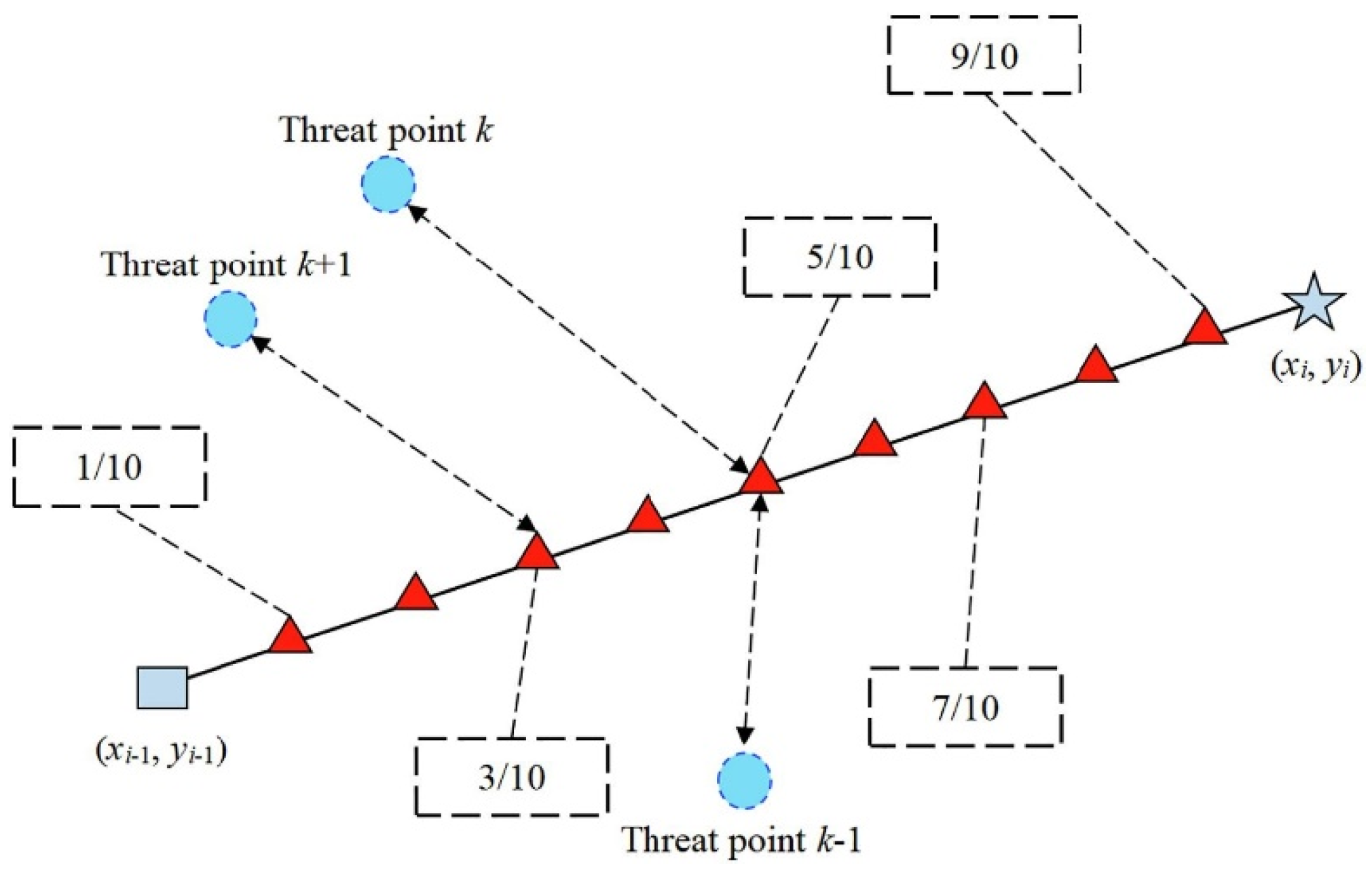
References
- Gong, C.; Zhou, N.; Xia, S.; Huang, S. Quantum particle swarm optimization algorithm based on diversity migration strategy. Future Gener. Comput. Syst. 2024, 157, 445–458. [Google Scholar] [CrossRef]
- Liu, Y.; As’ arry, A.; Hassan, M.K.; Hairuddin, A.A.; Mohamad, H. Review of the grey wolf optimization algorithm: Variants and applications. Neural Comput. Appl. 2024, 36, 2713–2735. [Google Scholar] [CrossRef]
- Kumar, A.; Nadeem, M.; Banka, H. Nature inspired optimization algorithms: A comprehensive overview. Evol. Syst. 2023, 14, 141–156. [Google Scholar] [CrossRef]
- Niu, Y.; Yan, X.; Wang, Y.; Niu, Y. An improved sand cat swarm optimization for moving target search by UAV. Expert Syst. Appl. 2024, 238, 122189. [Google Scholar] [CrossRef]
- Fu, S.; Li, K.; Huang, H.; Ma, C.; Fan, Q.; Zhu, Y. Red-billed blue magpie optimizer: A novel metaheuristic algorithm for 2D/3D UAV path planning and engineering design problems. Artif. Intell. Rev. 2024, 57, 1–89. [Google Scholar] [CrossRef]
- Duankhan, P.; Sunat, K.; Chiewchanwattana, S.; Nasa-Ngium, P. The Differentiated Creative Search (DCS): Leveraging differentiated knowledge-acquisition and creative realism to address complex optimization problems. Expert Syst. Appl. 2024, 252, 123734. [Google Scholar] [CrossRef]
- Kaur, S.; Kumar, Y.; Koul, A.; Kumar Kamboj, S. A systematic review on metaheuristic optimization techniques for feature selections in disease diagnosis: Open issues and challenges. Arch. Comput. Methods Eng. 2023, 30, 1863–1895. [Google Scholar] [CrossRef]
- Cui, J.; Wu, L.; Huang, X.; Xu, D.; Liu, C.; Xiao, W. Multi-strategy adaptable ant colony optimization algorithm and its application in robot path planning. Knowl. Based Syst. 2024, 288, 111459. [Google Scholar] [CrossRef]
- Abdel-Salam, M.; Houssein, E.H.; Emam, M.M.; Samee, N.A.; Jamjoom, M.M.; Hu, G. An adaptive enhanced human memory algorithm for multi-level image segmentation for pathological lung cancer images. Comput. Biol. Med. 2024, 183, 109272. [Google Scholar] [CrossRef]
- Xia, D.; Shen, B.; Zheng, Y.; Zhang, W.; Bai, D.; Hu, Y.; Li, H. A bidirectional-a-star-based ant colony optimization algorithm for big-data-driven taxi route recommendation. Multimed. Tools Appl. 2024, 83, 16313–16335. [Google Scholar] [CrossRef]
- Askr, H.; Abdel-Salam, M.; Snášel, V.; Hassanien, A.E. A green hydrogen production model from solar powered water electrolyze based on deep chaotic Lévy gazelle optimization. Eng. Sci. Technol. Int. J. 2024, 60, 101874. [Google Scholar] [CrossRef]
- Xu, X.-F.; Wang, K.; Ma, W.-H.; Wu, C.-L.; Huang, X.-R.; Ma, Z.-X.; Li, Z.-H. Multi-objective particle swarm optimization algorithm based on multi-strategy improvement for hybrid energy storage optimization configuration. Renew. Energy 2024, 223, 120086. [Google Scholar] [CrossRef]
- Elhosseny, M.; Abdel-salam, M.; Yang, J.; El-Hasnony, I.M. OLMM: An Optimized Lightweight Multiscale Model for Efficient Human Activity Recognition in IoT Consumer Applications. IEEE Trans. Consum. Electron. 2025. [Google Scholar] [CrossRef]
- Abdel-salam, M.; Hassanien, A.E.; Abdel-salam, M.; Hassanien, A.E. A Novel Dynamic Chaotic Golden Jackal Optimization Algorithm for Sensor-Based Human Activity Recognition Using Smartphones for Sustainable Smart Cities. In Artificial Intelligence for Environmental Sustainability and Green Initiatives; Springer: Berlin/Heidelberg, Germany, 2024; pp. 273–296. [Google Scholar]
- Ozkaya, B.; Duman, S.; Kahraman, H.T.; Guvenc, U. Optimal solution of the combined heat and power economic dispatch problem by adaptive fitness-distance balance based artificial rabbits optimization algorithm. Expert Syst. Appl. 2024, 238, 122272. [Google Scholar] [CrossRef]
- Abdel-Salam, M.; Chhabra, A.; Braik, M.; Gharehchopogh, F.S.; Bacanin, N. A Halton Enhanced Solution-based Human Evolutionary Algorithm for Complex Optimization and Advanced Feature Selection Problems. Knowl. Based Syst. 2025, 311, 113062. [Google Scholar] [CrossRef]
- Abdel-salam, M.; Alomari, S.A.; Almomani, M.H.; Hu, G.; Lee, S.; Saleem, K.; Smerat, A.; Abualigah, L. Quadruple strategy-driven hiking optimization algorithm for low and high-dimensional feature selection and real-world skin cancer classification. Knowl. Based Syst. 2025, 315, 113286. [Google Scholar] [CrossRef]
- Mostafa, R.R.; Hussien, A.G.; Gaheen, M.A.; Ewees, A.A.; Hashim, F.A. AEOWOA: Hybridizing whale optimization algorithm with artificial ecosystem-based optimization for optimal feature selection and global optimization. Evol. Syst. 2024, 15, 1753–1785. [Google Scholar] [CrossRef]
- Mostafa, R.R.; Hashim, F.A.; Chhabra, A.; Manita, G.; Xiao, Y. Empowering bonobo optimizer for global optimization and cloud scheduling problem. Clust. Comput. 2024, 27, 14557–14584. [Google Scholar] [CrossRef]
- Sharma, S.; Kumar, V.; Dutta, K. Multi-objective optimization algorithms for intrusion detection in IoT networks: A systematic review. Internet Things Cyber-Phys. Syst. 2024, 4, 258–267. [Google Scholar] [CrossRef]
- Aljehane, N.O.; Mengash, H.A.; Eltahir, M.M.; Alotaibi, F.A.; Aljameel, S.S.; Yafoz, A.; Alsini, R.; Assiri, M. Golden jackal optimization algorithm with deep learning assisted intrusion detection system for network security. Alex. Eng. J. 2024, 86, 415–424. [Google Scholar] [CrossRef]
- Saleem, S.; Hussain, F.; Baloch, N.K. IWO-IGA—A hybrid whale optimization algorithm featuring improved genetic characteristics for mapping real-time applications onto 2D network on chip. Algorithms 2024, 17, 115. [Google Scholar] [CrossRef]
- Elhosseny, M.; Abdel-Salam, M.; El-Hasnony, I.M. Adaptive dynamic crayfish algorithm with multi-enhanced strategy for global high-dimensional optimization and real-engineering problems. Sci. Rep. 2025, 15, 10656. [Google Scholar] [CrossRef] [PubMed]
- Abdel-Salam, M.; Alomari, S.A.; Yang, J.; Lee, S.; Saleem, K.; Smerat, A.; Snasel, V.; Abualigah, L. Harnessing dynamic turbulent dynamics in parrot optimization algorithm for complex high-dimensional engineering problems. Comput. Methods Appl. Mech. Eng. 2025, 440, 117908. [Google Scholar] [CrossRef]
- Saemi, B.; Goodarzian, F. Energy-efficient routing protocol for underwater wireless sensor networks using a hybrid metaheuristic algorithm. Eng. Appl. Artif. Intell. 2024, 133, 108132. [Google Scholar] [CrossRef]
- Yan, Z.; Yan, J.; Wu, Y.; Cai, S.; Wang, H. A novel reinforcement learning based tuna swarm optimization algorithm for autonomous underwater vehicle path planning. Math. Comput. Simul. 2023, 209, 55–86. [Google Scholar] [CrossRef]
- Yahia, H.S.; Mohammed, A.S. Path planning optimization in unmanned aerial vehicles using meta-heuristic algorithms: A systematic review. Environ. Monit. Assess. 2023, 195, 30. [Google Scholar] [CrossRef]
- Mirjalili, S.; Mirjalili, S.M.; Lewis, A. Grey wolf optimizer. Adv. Eng. Softw. 2014, 69, 46–61. [Google Scholar] [CrossRef]
- Kennedy, J.; Eberhart, R. Particle swarm optimization. In Proceedings of the ICNN’95-International Conference on Neural Networks, Perth, WA, Australia, 27 November–1 December 1995; pp. 1942–1948. [Google Scholar]
- Heidari, A.A.; Mirjalili, S.; Faris, H.; Aljarah, I.; Mafarja, M.; Chen, H. Harris hawks optimization: Algorithm and applications. Future Gener. Comput. Syst. 2019, 97, 849–872. [Google Scholar] [CrossRef]
- Mirjalili, S.; Lewis, A. The whale optimization algorithm. Adv. Eng. Softw. 2016, 95, 51–67. [Google Scholar] [CrossRef]
- Faramarzi, A.; Heidarinejad, M.; Mirjalili, S.; Gandomi, A.H. Marine Predators Algorithm: A nature-inspired metaheuristic. Expert Syst. Appl. 2020, 152, 113377. [Google Scholar] [CrossRef]
- Xue, J.; Shen, B. A novel swarm intelligence optimization approach: Sparrow search algorithm. Syst. Sci. Control Eng. 2020, 8, 22–34. [Google Scholar] [CrossRef]
- Dehghani, M.; Hubálovský, Š.; Trojovský, P. Northern goshawk optimization: A new swarm-based algorithm for solving optimization problems. IEEE Access 2021, 9, 162059–162080. [Google Scholar] [CrossRef]
- Minh, H.-L.; Sang-To, T.; Theraulaz, G.; Wahab, M.A.; Cuong-Le, T. Termite life cycle optimizer. Expert Syst. Appl. 2023, 213, 119211. [Google Scholar] [CrossRef]
- Storn, R.; Price, K. Differential evolution–a simple and efficient heuristic for global optimization over continuous spaces. J. Glob. Optim. 1997, 11, 341–359. [Google Scholar] [CrossRef]
- Jeong, I.-K.; Lee, J.-J. Adaptive simulated annealing genetic algorithm for system identification. Eng. Appl. Artif. Intell. 1996, 9, 523–532. [Google Scholar] [CrossRef]
- Han, K.-H.; Kim, J.-H. Quantum-inspired evolutionary algorithm for a class of combinatorial optimization. IEEE Trans. Evol. Comput. 2002, 6, 580–593. [Google Scholar] [CrossRef]
- Iruthayarajan, M.W.; Baskar, S. Covariance matrix adaptation evolution strategy based design of centralized PID controller. Expert Syst. Appl. 2010, 37, 5775–5781. [Google Scholar] [CrossRef]
- Mirjalili, S. SCA: A sine cosine algorithm for solving optimization problems. Knowl. Based Syst. 2016, 96, 120–133. [Google Scholar] [CrossRef]
- Rashedi, E.; Nezamabadi-Pour, H.; Saryazdi, S. GSA: A gravitational search algorithm. Inf. Sci. 2009, 179, 2232–2248. [Google Scholar] [CrossRef]
- Minh, H.-L.; Sang-To, T.; Wahab, M.A.; Cuong-Le, T. A new metaheuristic optimization based on K-means clustering algorithm and its application to structural damage identification. Knowl. Based Syst. 2022, 251, 109189. [Google Scholar] [CrossRef]
- Zhao, W.; Wang, L.; Zhang, Z. Atom search optimization and its application to solve a hydrogeologic parameter estimation problem. Knowl. Based Syst. 2019, 163, 283–304. [Google Scholar] [CrossRef]
- Wolpert, D.H.; Macready, W.G. No free lunch theorems for optimization. IEEE Trans. Evol. Comput. 1997, 1, 67–82. [Google Scholar] [CrossRef]
- Meng, Z.; Yang, C.; Li, X.; Chen, Y. Di-DE: Depth information-based differential evolution with adaptive parameter control for numerical optimization. IEEE Access 2020, 8, 40809–40827. [Google Scholar] [CrossRef]
- Gao, Z.-M.; Zhao, J. An improved grey wolf optimization algorithm with variable weights. Comput. Intell. Neurosci. 2019, 2019, 2981282. [Google Scholar] [CrossRef] [PubMed]
- Das, P.K.; Behera, H.S.; Panigrahi, B.K. A hybridization of an improved particle swarm optimization and gravitational search algorithm for multi-robot path planning. Swarm Evol. Comput. 2016, 28, 14–28. [Google Scholar] [CrossRef]
- Naik, M.K.; Jena, B.; Patra, G.R.; Wunnava, A. Dombi entropy based multilevel thresholding of Liver CT scan images using leader slime mould algorithm. In Proceedings of the 2023 2nd International Conference on Ambient Intelligence in Health Care (ICAIHC), Online, 17–18 November 2023; pp. 1–6. [Google Scholar]
- Ball, A.K.; Zhou, K.; Xu, D.; Zhang, D.; Tang, J. Directed Gaussian process metamodeling with improved firefly algorithm (iFA) for composite manufacturing uncertainty propagation analysis. Int. J. Adv. Manuf. Technol. 2023, 126, 49–66. [Google Scholar] [CrossRef]
- Gharehchopogh, F.S.; Abdollahzadeh, B. An efficient harris hawk optimization algorithm for solving the travelling salesman problem. Clust. Comput. 2022, 25, 1981–2005. [Google Scholar] [CrossRef]
- Akopov, A.S. MBHGA: A matrix-based hybrid genetic algorithm for solving an agent-based model of controlled trade interactions. IEEE Access 2025, 13, 26843–26863. [Google Scholar] [CrossRef]
- Madushani, Y.; Kasthurirathna, D. Incorporating strategy adoption into genetic algorithm enabled multi-agent systems. In Proceedings of the 2020 IEEE Congress on Evolutionary Computation (CEC), Glasgow, UK, 19–24 July 2020; pp. 1–8. [Google Scholar]
- Wang, X.; Dong, X.; Zhang, Y.; Chen, H. Crisscross Harris hawks optimizer for global tasks and feature selection. J. Bionic Eng. 2023, 20, 1153–1174. [Google Scholar] [CrossRef]
- Chakraborty, S.; Saha, A.K.; Ezugwu, A.E.; Chakraborty, R.; Saha, A. Horizontal crossover and co-operative hunting-based Whale Optimization Algorithm for feature selection. Knowl. Based Syst. 2023, 282, 111108. [Google Scholar] [CrossRef]
- Izci, D.; Ekinci, S.; Rizk-Allah, R.M.; Alribdi, N.I.; Smerat, A.; Alzahrani, A.; Alwadain, A.; Snasel, V.; Abualigah, L. Master–Slave Architecture Enhanced and Improved GBO Tuned Cascaded PI-PDN Controller for Speed Regulation of DC Motors. Optim. Control Appl. Methods 2025. [Google Scholar] [CrossRef]
- Izci, D.; Ekinci, S.; Kayri, M.; Eker, E. A novel improved arithmetic optimization algorithm for optimal design of PID controlled and Bode’s ideal transfer function based automobile cruise control system. Evol. Syst. 2022, 13, 453–468. [Google Scholar] [CrossRef]
- Ghasemi, M.; Zare, M.; Trojovský, P.; Rao, R.V.; Trojovská, E.; Kandasamy, V. Optimization based on the smart behavior of plants with its engineering applications: Ivy algorithm. Knowl. Based Syst. 2024, 295, 111850. [Google Scholar] [CrossRef]
- Meng, A.-b.; Chen, Y.-c.; Yin, H.; Chen, S.-z. Crisscross optimization algorithm and its application. Knowl. Based Syst. 2014, 67, 218–229. [Google Scholar] [CrossRef]
- Xue, J.; Shen, B. Dung beetle optimizer: A new meta-heuristic algorithm for global optimization. J. Supercomput. 2023, 79, 7305–7336. [Google Scholar] [CrossRef]
- Mohamed, A.W.; Hadi, A.A.; Fattouh, A.M.; Jambi, K.M. LSHADE with semi-parameter adaptation hybrid with CMA-ES for solving CEC 2017 benchmark problems. In Proceedings of the 2017 IEEE Congress on evolutionary computation (CEC), San Sebastian, Spain, 5–8 June 2017; pp. 145–152. [Google Scholar]
- Luo, W.; Lin, X.; Li, C.; Yang, S.; Shi, Y. Benchmark functions for CEC 2022 competition on seeking multiple optima in dynamic environments. arXiv 2022, arXiv:2201.00523. [Google Scholar] [CrossRef]
- Abualigah, L.; Diabat, A.; Mirjalili, S.; Abd Elaziz, M.; Gandomi, A.H. The arithmetic optimization algorithm. Comput. Methods Appl. Mech. Eng. 2021, 376, 113609. [Google Scholar] [CrossRef]
- Abdel-Basset, M.; Mohamed, R.; Jameel, M.; Abouhawwash, M. Spider wasp optimizer: A novel meta-heuristic optimization algorithm. Artif. Intell. Rev. 2023, 56, 11675–11738. [Google Scholar] [CrossRef]
- Dehghani, M.; Montazeri, Z.; Trojovská, E.; Trojovský, P. Coati Optimization Algorithm: A new bio-inspired metaheuristic algorithm for solving optimization problems. Knowl. Based Syst. 2023, 259, 110011. [Google Scholar] [CrossRef]
- Jia, H.; Rao, H.; Wen, C.; Mirjalili, S. Crayfish optimization algorithm. Artif. Intell. Rev. 2023, 56, 1919–1979. [Google Scholar] [CrossRef]
- Zhao, S.; Zhang, T.; Ma, S.; Wang, M. Sea-horse optimizer: A novel nature-inspired meta-heuristic for global optimization problems. Appl. Intell. 2023, 53, 11833–11860. [Google Scholar] [CrossRef]
- Chopra, N.; Ansari, M.M. Golden jackal optimization: A novel nature-inspired optimizer for engineering applications. Expert Syst. Appl. 2022, 198, 116924. [Google Scholar] [CrossRef]
- Zhu, D.; Wang, S.; Zhou, C.; Yan, S.; Xue, J. Human memory optimization algorithm: A memory-inspired optimizer for global optimization problems. Expert Syst. Appl. 2024, 237, 121597. [Google Scholar] [CrossRef]
- Houssein, E.H.; Hammad, A.; Emam, M.M.; Ali, A.A. An enhanced Coati Optimization Algorithm for global optimization and feature selection in EEG emotion recognition. Comput. Biol. Med. 2024, 173, 108329. [Google Scholar] [CrossRef] [PubMed]
- Long, W.; Cai, S.; Jiao, J.; Xu, M.; Wu, T. A new hybrid algorithm based on grey wolf optimizer and cuckoo search for parameter extraction of solar photovoltaic models. Energy Convers. Manag. 2020, 203, 112243. [Google Scholar] [CrossRef]
- Chen, H.; Yang, C.; Heidari, A.A.; Zhao, X. An efficient double adaptive random spare reinforced whale optimization algorithm. Expert Syst. Appl. 2020, 154, 113018. [Google Scholar] [CrossRef]
- Hu, G.; Zhong, J.; Du, B.; Wei, G. An enhanced hybrid arithmetic optimization algorithm for engineering applications. Comput. Methods Appl. Mech. Eng. 2022, 394, 114901. [Google Scholar] [CrossRef]
- Khodadadi, N.; Snasel, V.; Mirjalili, S. Dynamic arithmetic optimization algorithm for truss optimization under natural frequency constraints. IEEE Access 2022, 10, 16188–16208. [Google Scholar] [CrossRef]
- Wu, H.; Zhang, A.; Han, Y.; Nan, J.; Li, K. Fast stochastic configuration network based on an improved sparrow search algorithm for fire flame recognition. Knowl. Based Syst. 2022, 245, 108626. [Google Scholar] [CrossRef]
- Brest, J.; Greiner, S.; Boskovic, B.; Mernik, M.; Zumer, V. Self-adapting control parameters in differential evolution: A comparative study on numerical benchmark problems. IEEE Trans. Evol. Comput. 2006, 10, 646–657. [Google Scholar] [CrossRef]
- Rather, S.A.; Bala, P.S. Hybridization of constriction coefficient based particle swarm optimization and gravitational search algorithm for function optimization. In Proceedings of the International Conference on Advances in Electronics, Electrical & Computational Intelligence (ICAEEC), Prayagraj, India, 31 May–1 June 2019. [Google Scholar]
- Fu, Y.; Liu, D.; Chen, J.; He, L. Secretary bird optimization algorithm: A new metaheuristic for solving global optimization problems. Artif. Intell. Rev. 2024, 57, 123. [Google Scholar] [CrossRef]
- Abdollahzadeh, B.; Khodadadi, N.; Barshandeh, S.; Trojovský, P.; Gharehchopogh, F.S.; El-kenawy, E.-S.M.; Abualigah, L.; Mirjalili, S. Puma optimizer (PO): A novel metaheuristic optimization algorithm and its application in machine learning. Clust. Comput. 2024, 27, 5235–5283. [Google Scholar] [CrossRef]
- Siegel, S.; Castellan, N. The Friedman Two-Way Analysis of Variance by Ranks. Nonparametric Statistics for the Behavioral Sciences; McGraw-Hill: New York, NY, USA, 1988; pp. 174–184. [Google Scholar] [CrossRef]
- Derrac, J.; García, S.; Molina, D.; Herrera, F. A practical tutorial on the use of nonparametric statistical tests as a methodology for comparing evolutionary and swarm intelligence algorithms. Swarm Evol. Comput. 2011, 1, 3–18. [Google Scholar] [CrossRef]
- Song, S.; Zhang, K.; Zhang, L.; Wu, N. A dual-population algorithm based on self-adaptive epsilon method for constrained multi-objective optimization. Inf. Sci. 2024, 655, 119906. [Google Scholar] [CrossRef]
- Rezaei, K.; Fard, O.S. Multi-strategy enhanced Marine Predators Algorithm with applications in engineering optimization and feature selection problems. Appl. Soft Comput. 2024, 159, 111650. [Google Scholar] [CrossRef]
- El-Kenawy, E.-S.M.; Khodadadi, N.; Mirjalili, S.; Abdelhamid, A.A.; Eid, M.M.; Ibrahim, A. Greylag goose optimization: Nature-inspired optimization algorithm. Expert Syst. Appl. 2024, 238, 122147. [Google Scholar] [CrossRef]
- Wang, S.; Cao, L.; Chen, Y.; Chen, C.; Yue, Y.; Zhu, W. Gorilla optimization algorithm combining sine cosine and cauchy variations and its engineering applications. Sci. Rep. 2024, 14, 7578. [Google Scholar] [CrossRef]
- Zarbilinezhad, M.; Gholizad, A. Hybrid optimization algorithm based on chaos game and differential evolution for constrained optimization of structures. Eng. Optim. 2024, 1–32. [Google Scholar] [CrossRef]
- Hu, G.; Zhong, J.; Wei, G. SaCHBA_PDN: Modified honey badger algorithm with multi-strategy for UAV path planning. Expert Syst. Appl. 2023, 223, 119941. [Google Scholar] [CrossRef]
- Arora, S.; Singh, S. Butterfly optimization algorithm: A novel approach for global optimization. Soft Comput. 2019, 23, 715–734. [Google Scholar] [CrossRef]
- Kaur, S.; Awasthi, L.K.; Sangal, A.; Dhiman, G. Tunicate Swarm Algorithm: A new bio-inspired based metaheuristic paradigm for global optimization. Eng. Appl. Artif. Intell. 2020, 90, 103541. [Google Scholar] [CrossRef]
- Shen, Q.; Zhang, D.; Xie, M.; He, Q. Multi-strategy enhanced dung beetle optimizer and its application in three-dimensional UAV path planning. Symmetry 2023, 15, 1432. [Google Scholar] [CrossRef]
- Yuxuan, X.; Sun, Z.; Yuan, K.; Sun, Z. 3D UAV Route Optimization in Complex Environments Using an Enhanced Artificial Lemming Algorithm. Symmetry 2025, 17, 946. [Google Scholar] [CrossRef]

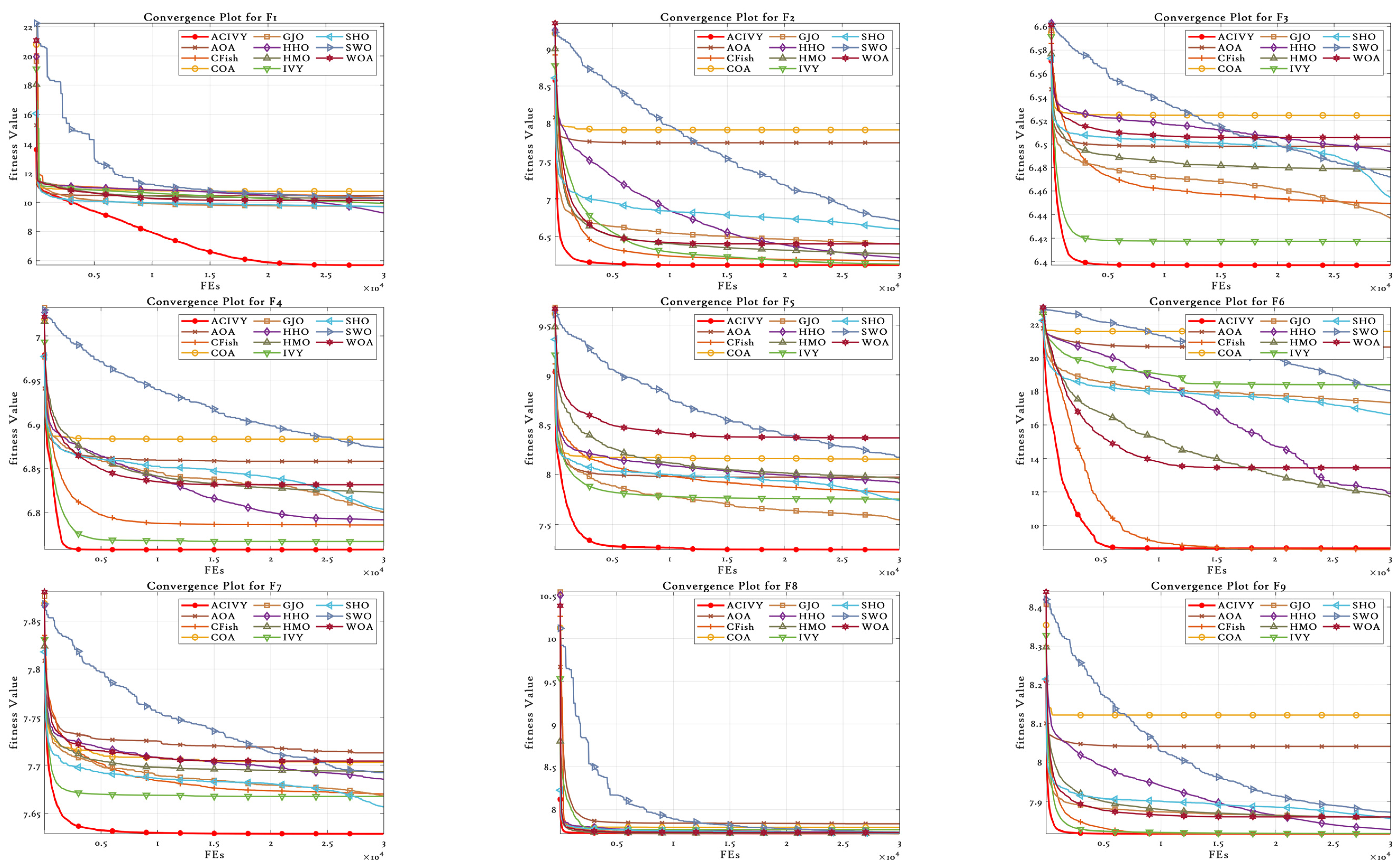
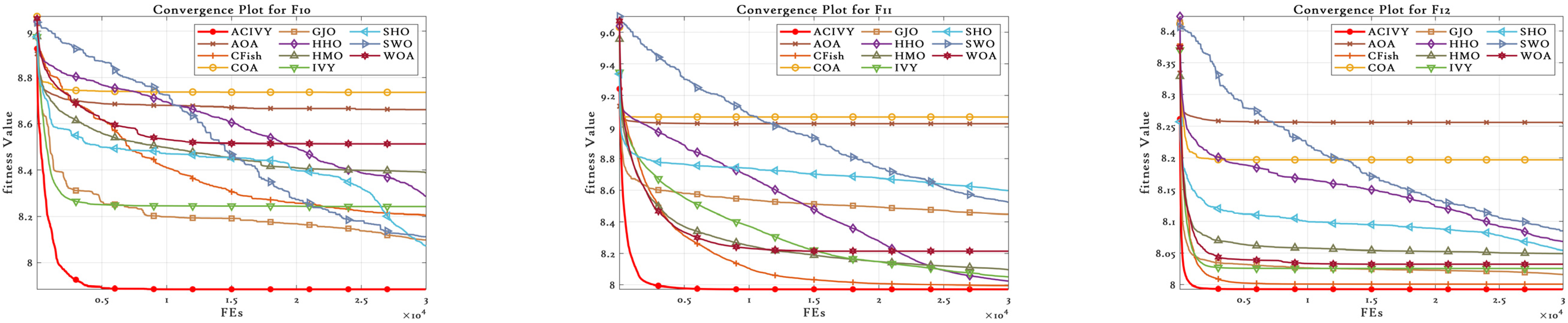
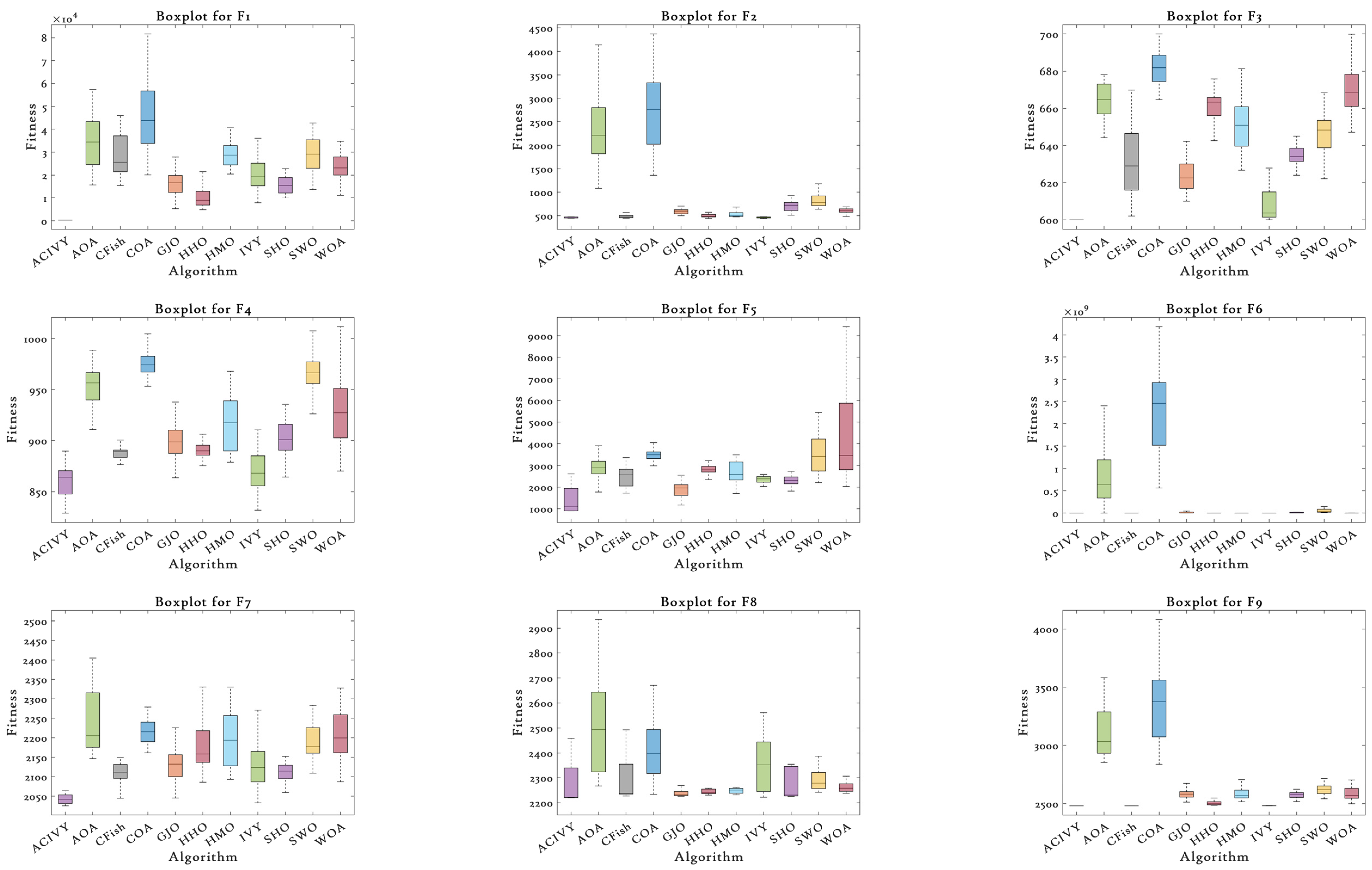
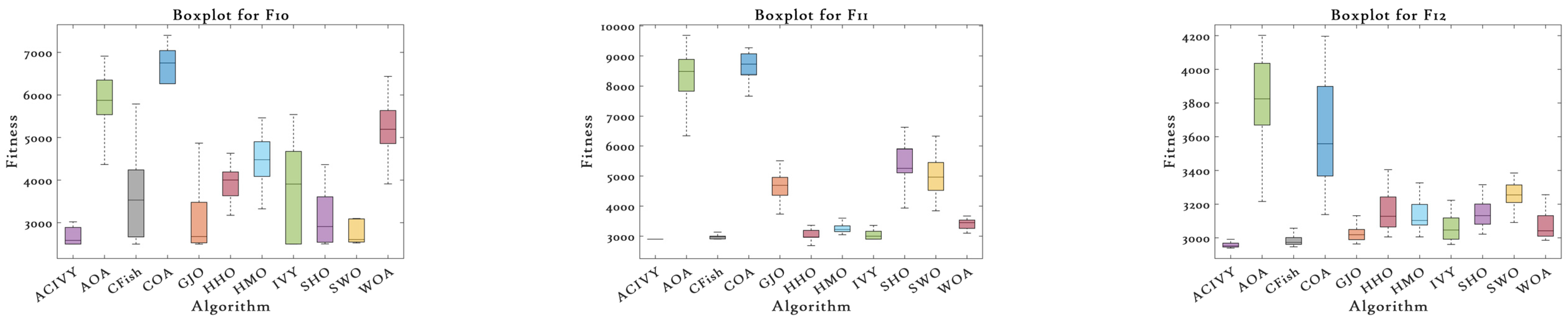
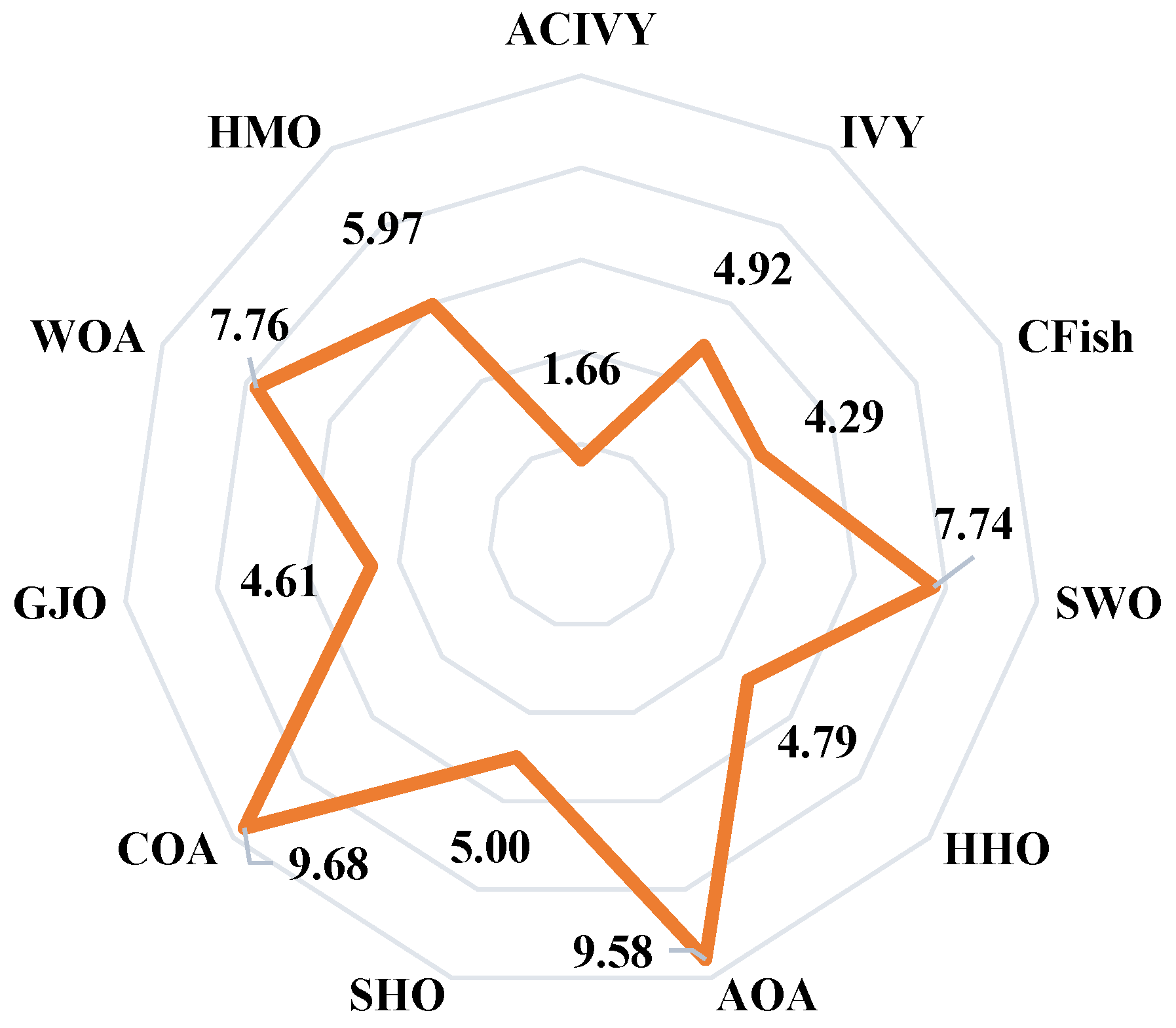
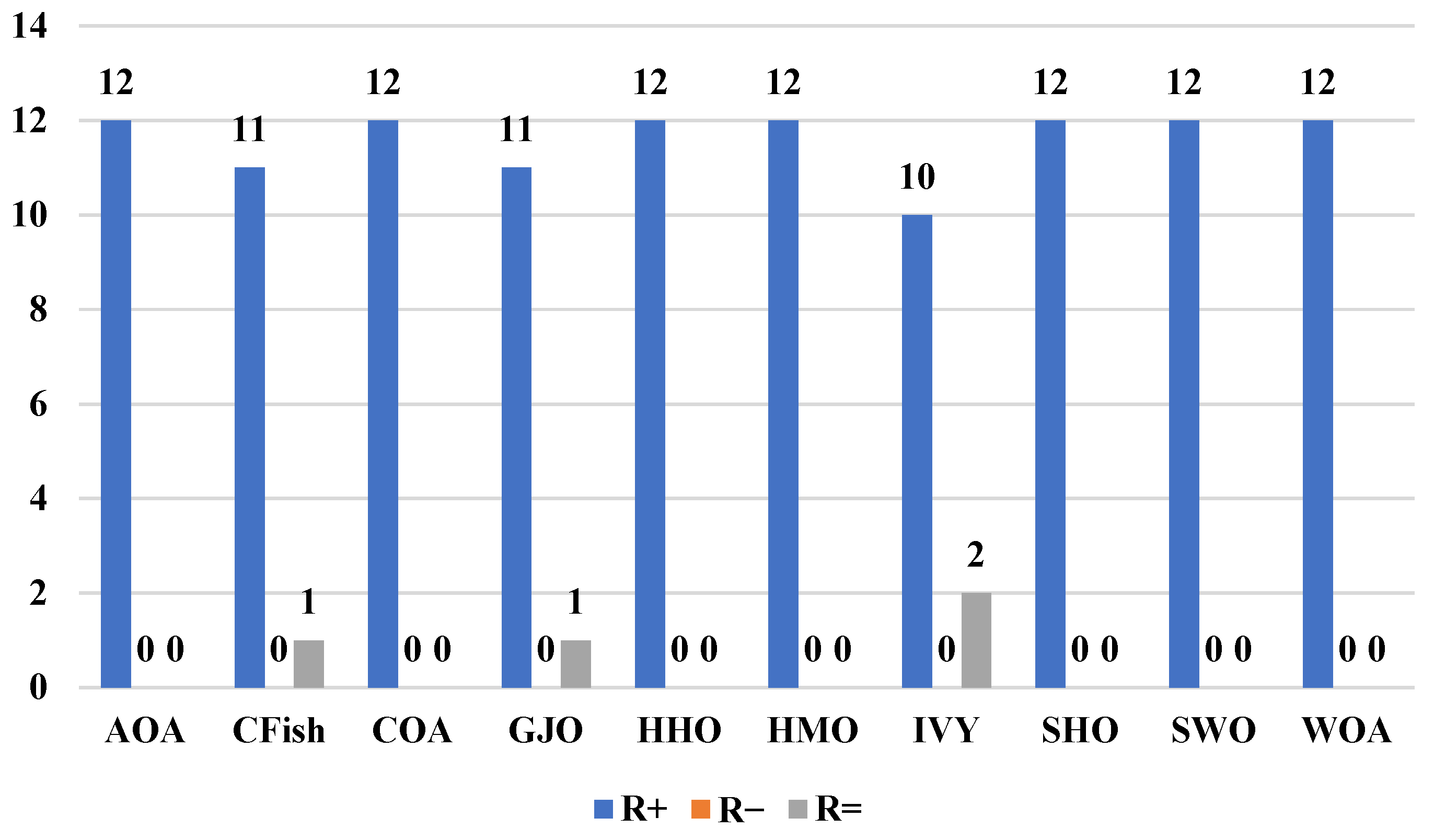
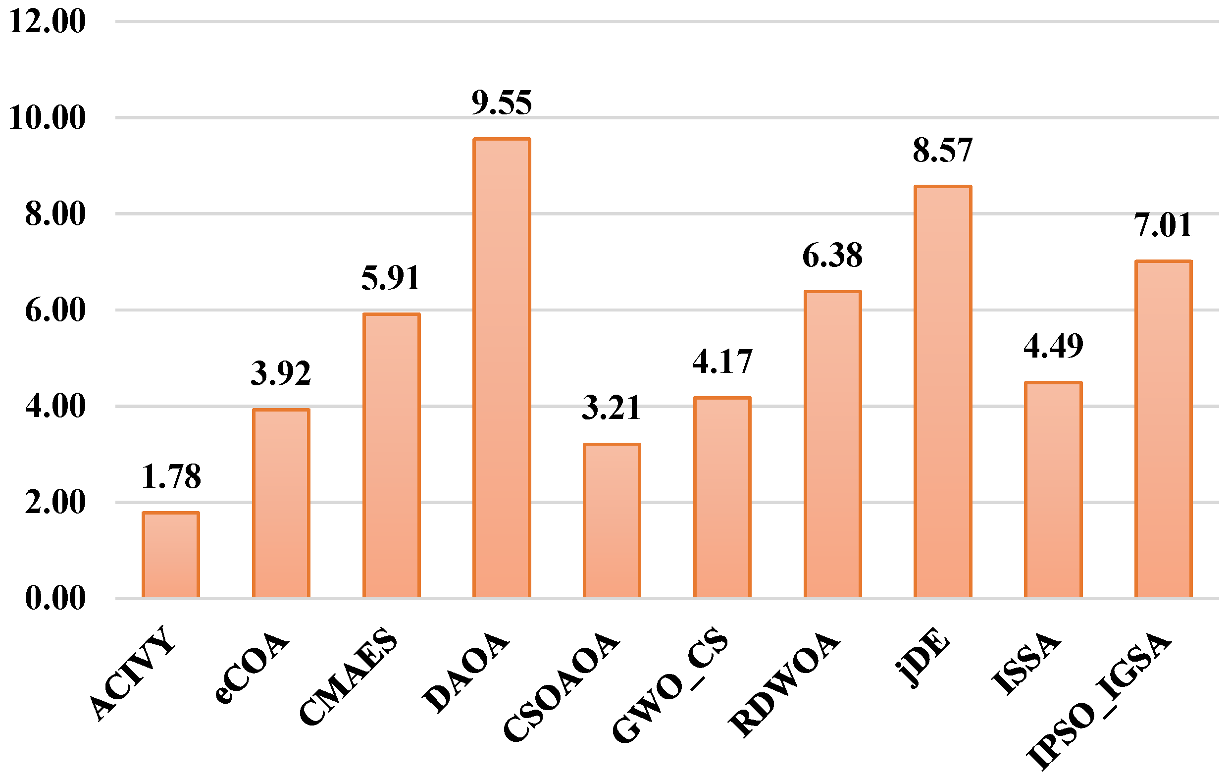
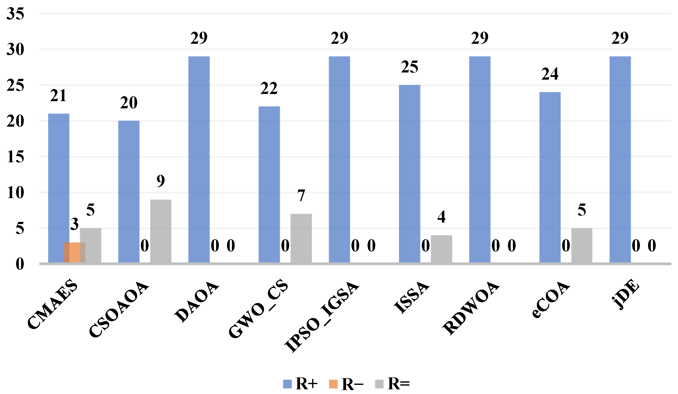

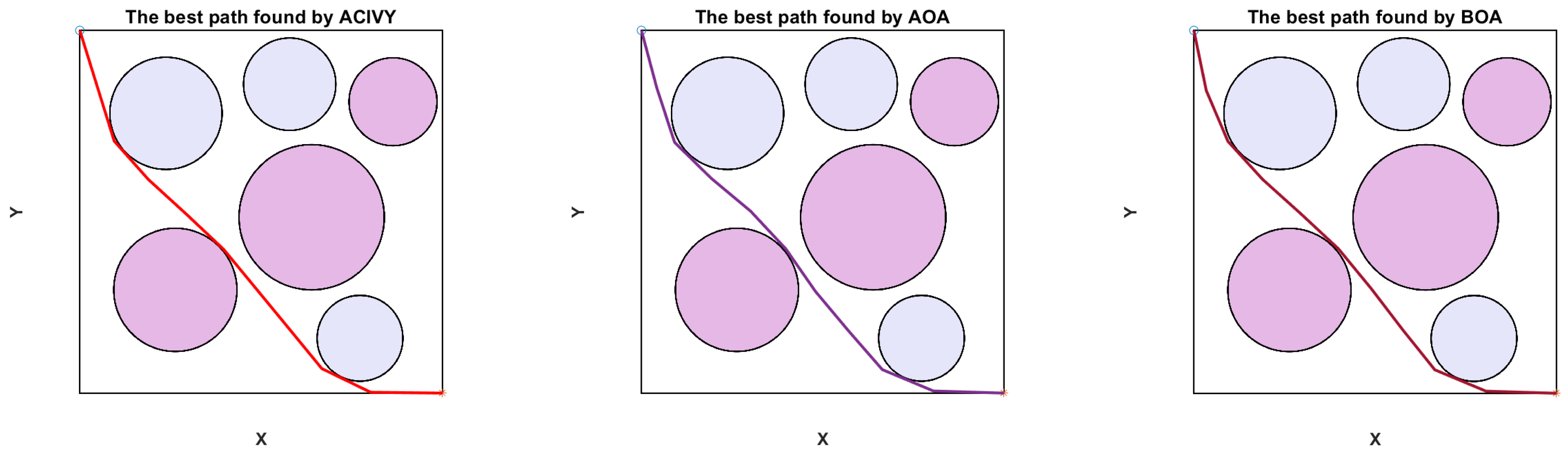
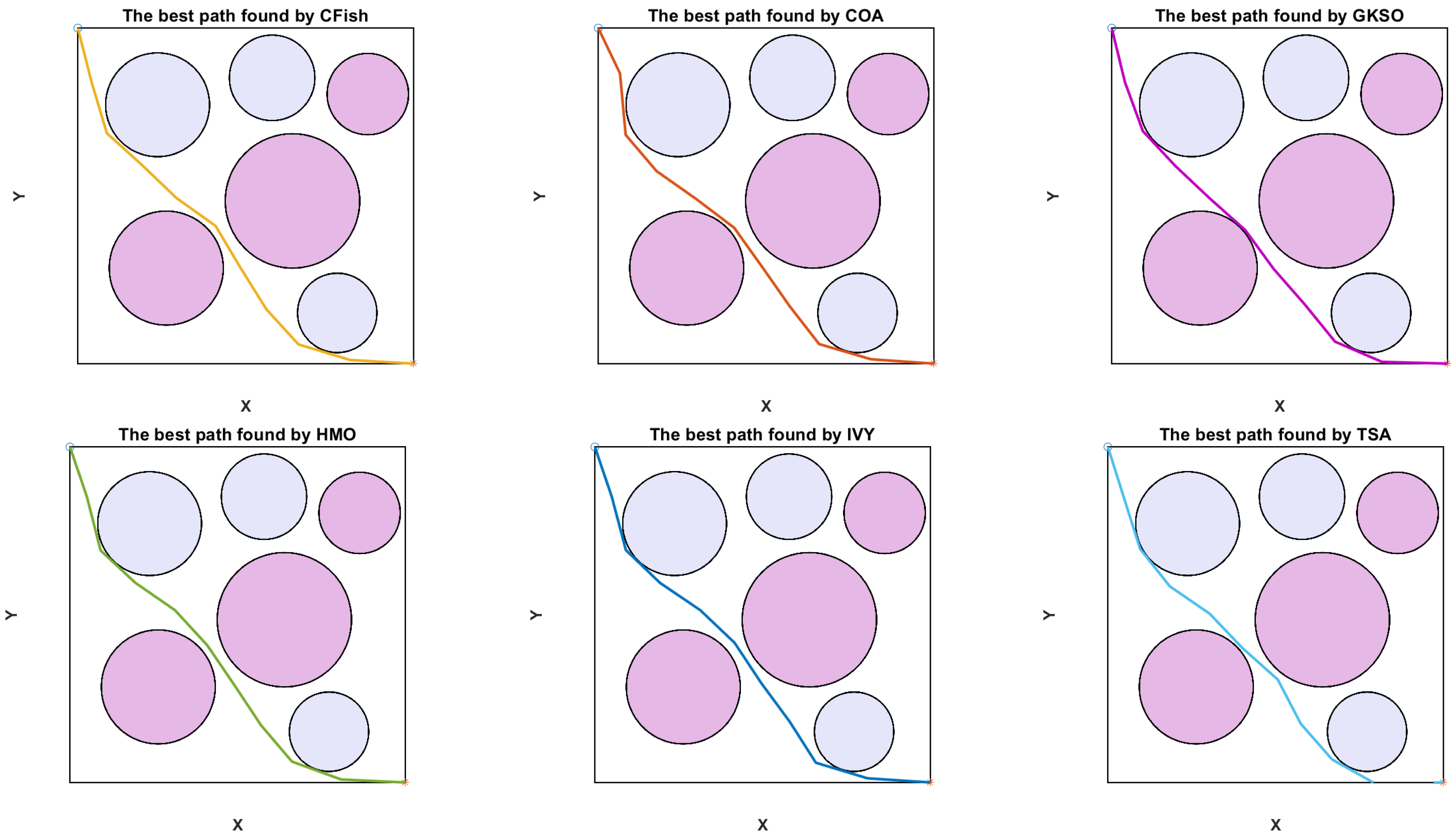

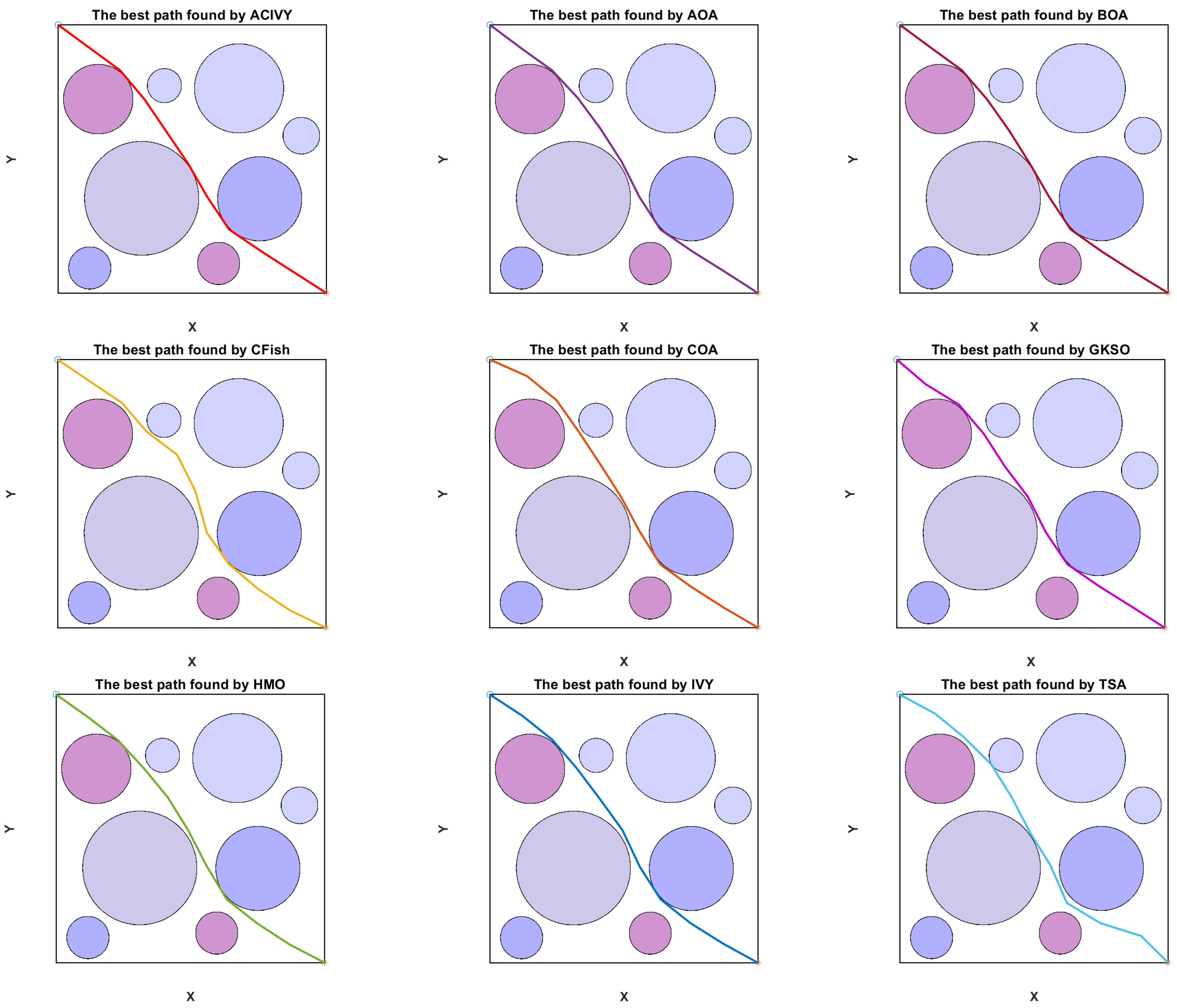

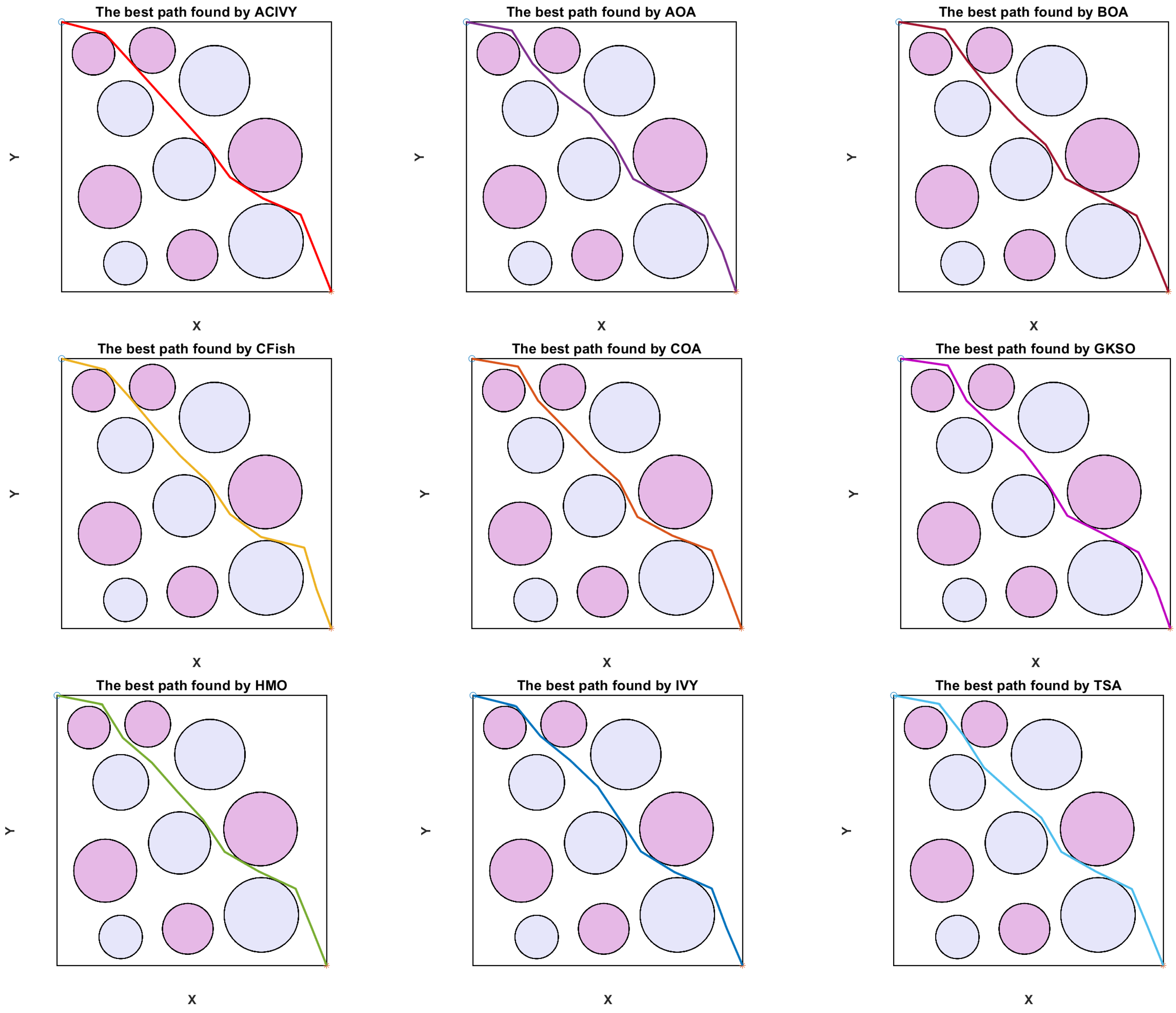
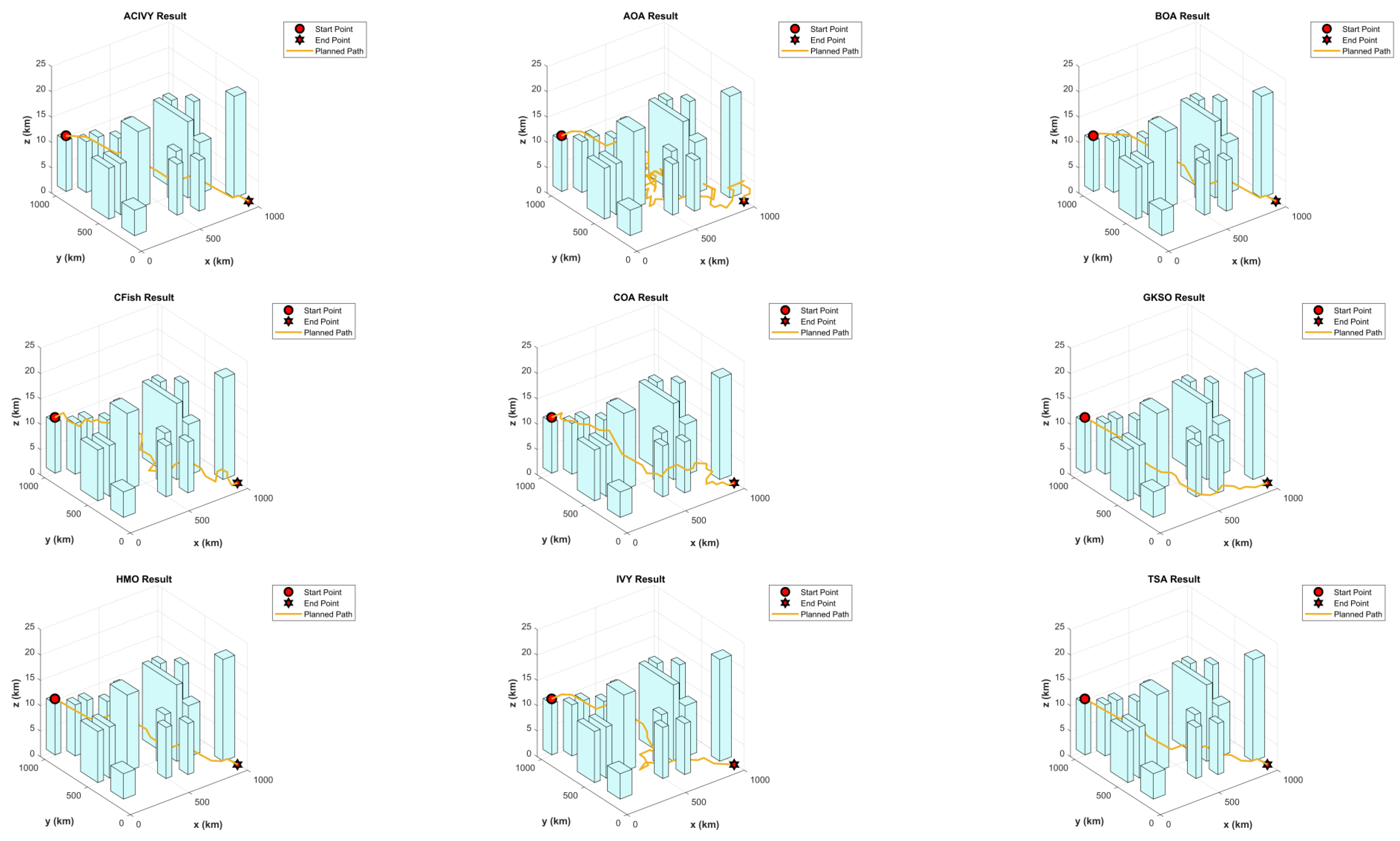
Disclaimer/Publisher’s Note: The statements, opinions and data contained in all publications are solely those of the individual author(s) and contributor(s) and not of MDPI and/or the editor(s). MDPI and/or the editor(s) disclaim responsibility for any injury to people or property resulting from any ideas, methods, instructions or products referred to in the content. |
© 2025 by the authors. Licensee MDPI, Basel, Switzerland. This article is an open access article distributed under the terms and conditions of the Creative Commons Attribution (CC BY) license (https://creativecommons.org/licenses/by/4.0/).