Author Contributions
Conceptualization, A.D., N.M., S.K., F.E.F. and J.L.T.; methodology, A.D., N.M. and S.K.; software, A.D.; validation, A.D., N.M. and S.K.; formal analysis, A.D. and S.K.; investigation, A.D. and N.M.; resources, J.L.T. and F.E.F.; data curation, A.D.; writing—original draft preparation, A.D.; writing—review and editing, A.D., N.M., S.K., F.E.F. and J.L.T.; visualization, A.D., N.M. and S.K.; supervision, J.L.T. and F.E.F.; project administration, J.L.T., F.E.F. and A.D.; funding acquisition, J.L.T. and F.E.F. All authors have read and agreed to the published version of the manuscript.
Figure 1.
California sea lion swimming and characteristic propulsive stroke. (A) Sea lion maneuvering underwater using its foreflippers, hind flippers, and body for agile control. (B) Sequential frames from underwater video showing the three phases of the characteristic foreflipper stroke: Recovery, during which the flippers extend laterally and anteriorly away from the body; Power, where the flippers move downward and medially to generate thrust; and Paddle, as the flippers are pulled posteriorly toward the body to complete the stroke cycle and reset for the next recovery phase.
Figure 2.
Anatomical coordinate system of the California sea lion. Body-fixed coordinate frame and associated anatomical planes used to describe foreflipper motion. The x-axis is oriented anteroposteriorly along the body midline toward the head, the y-axis extends laterally, and the z-axis extends dorsoventrally. These axes define the Sagittal (x − z), Transverse (y − z), and Dorsal (x − y) planes, which, respectively, separate the left and right sides, dorsal and ventral regions, and anterior and posterior portions of the body.
Figure 3.
Bio-robotic foreflipper coordinate system and actuation scheme. (A) The bio-robotic foreflipper replicates sea lion forelimb motion through three serially arranged actuators (flap, sweep, and twist). A flexible hinge at the wrist introduces passive bending representative of the biological joint (B) Representative actuator motions showing the range of rotation for each axis: flap angle (θf), sweep angle (θs), and twist angle (θt). The zero position aligns the flipper parallel to the body flank with the leading edge downward. Increasing actuator angles illustrate the independent and combined rotations that generate the full spatial envelope of sea lion foreflipper movement.
Figure 4.
Bio-robotic Single Flipper Robot. (A) CAD model of the single flipper robot with the actuatable axes labeled (B) Full bio-robotic single flipper robot with (Left) support structure, control box, and actuators and (Right) a closer view of the flipper and actuator set-up.
Figure 4.
Bio-robotic Single Flipper Robot. (A) CAD model of the single flipper robot with the actuatable axes labeled (B) Full bio-robotic single flipper robot with (Left) support structure, control box, and actuators and (Right) a closer view of the flipper and actuator set-up.
Figure 5.
Design Of Engineered Sea Lion Flipper. (A) Foreflipper bending during sea lion swimming; (B) 3D model of sea lion foreflipper showing bone structure; (C) Final design of foreflipper model, highlighting the two rigid sections cast in flexible silicon; (D) Foreflipper model bending during actuation.
Figure 6.
Experimental test environment. (A) Schematic, photograph, and computational fluid dynamics (CFD) simulation of the circulating flow tank used for experiments. Water is driven by dual propulsors and passes through three flow straighteners before entering the central test area. The CFD velocity map confirms uniform flow distribution and stable velocity profiles within the test region. (B) Experimental apparatus showing the suspended measurement system, including two-axis linear air bushings for low-friction translation, thrust and lift force sensors for load measurement, and the single bio-robotic foreflipper mounted within the test area. Green arrows represent flow direction.
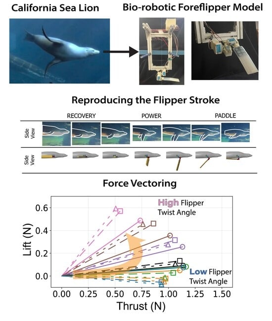
Figure 7.
Characteristic foreflipper stroke of the California sea lion and corresponding robotic implementation. (A) Sequential views of the biological and bio-robotic foreflipper illustrating the three primary phases of the characteristic propulsive stroke: Recovery, where the flipper moves upward and outward to a laterally extended position minimizing drag; Power, characterized by a strong downward and rearward motion that generates thrust; and Paddle, where the flipper moves ventrally toward the body while maintaining lift before returning to the streamlined position. The bio-robotic foreflipper reproduces these coordinated motions through flap (θf), sweep (θs), and twist (θt). (B) Parameterized joint trajectories for flap, sweep, and twist angles across one full stroke cycle, modeled using a piecewise cubic Hermite interpolating polynomial (PCHIP) fit to biological kinematic data. Together, these actuator profiles recreate the continuous, nonplanar motion and characteristic feathering of the sea lion’s foreflipper during propulsion.

Figure 8.
PCHIP spline representation of foreflipper kinematics. Parameterized flap (θf), sweep (θs), and twist (θt) angles over one complete stroke cycle, divided into the Recovery, Power, Paddle, and Reset phases. Red circles indicate control points defining the piecewise cubic Hermite interpolating polynomial (PCHIP) splines used to generate smooth, shape-preserving joint trajectories without overshoot. These control points can be adjusted to modify amplitude, timing, and phase relationships between the three motions, enabling controlled variation of stroke kinematics in experiments while faithfully reproducing the characteristic sea lion stroke observed in the animal.
Figure 9.
Time-varying thrust and lift traces for the baseline propulsive strokes. Thrust (top row) and lift (bottom row) are shown for: (A) the isolated power phase, (B) the isolated paddle phase, and (C) the combined power-paddle stroke. The horizontal axis is nondimensional time (t/T), and the vertical axis is force (N). For each trace, the horizontal dotted line indicates the mean force over the phase, and the vertical solid line marks the timing of the peak force.
Figure 10.
Effect of kinematic variations on isolated power phase forces. Time-varying thrust (top row) and lift (bottom row) traces are shown for manipulations of the baseline stroke. (A) Effect of varying the flipper twist angle (θt) from 0° to 90°. (B) Effect of varying the starting sweep angle (θs) from 70° to 90°. (C) Effect of the presence of oncoming flow (U). The horizontal axis is nondimensional time (t/T), and the vertical axis is force (N). The baseline (BL) condition is highlighted in each panel for reference.
Figure 11.
Summary of mean propulsive forces generated during the isolated power phase. Panel (A) illustrates the effect of varying the Twist Angle (θt) and Sweep Angle (θs) on mean Thrust (left) and mean Lift (middle) and Lift vs. Thrust vector (Bottom). Panel (B) illustrates the effect of varying the Twist Angle (θt) and Flow Speed (U) on mean Thrust (left) and mean Lift (middle) and Lift vs. Thrust.
Figure 12.
Peak magnitude and peak timing for the isolated power phase. Peak force magnitude (N, y-axis) is plotted against nondimensional peak timing (t/T, x-axis) for both peak thrust (top row) and peak lift (bottom row). (A) Illustrates the effect of varying the Twist Angle (θt) and Sweep Angle (θs). (B) Illustrates the effect of varying the Twist Angle (θt) and Flow Speed (U). The baseline condition is identified by the red square.
Figure 13.
Effect of kinematic variations on isolated paddle phase forces. Time-varying thrust (top row) and lift (bottom row) traces are shown for manipulations of the baseline stroke. (A) Effect of varying the flipper twist angle (θt) from 0° to 90°. (B) Effect of varying the starting sweep angle (θs) from 70° to 90°. (C) Effect of the presence of oncoming flow (U). The horizontal axis is nondimensional time (t/T), and the vertical axis is force (N). The baseline (BL) condition is highlighted in each panel for reference.
Figure 14.
Summary of mean propulsive forces generated during the isolated paddle phase. Panel (A) illustrates the effect of varying the Twist Angle (θt) and Sweep Angle (θs) on mean Thrust (left) and mean Lift (middle) and Lift vs. Thrust vector (Bottom) Panel (B) illustrates the effect of varying the Twist Angle (θt) and Flow Speed (U) on mean Thrust (left) and mean Lift (middle) and Lift vs. Thrust.
Figure 15.
Peak magnitude and peak timing for the isolated paddle phase. Peak force magnitude (N, y-axis) is plotted against nondimensional peak timing (t/T, x-axis) for both peak thrust (top row) and peak lift (bottom row). (A) Illustrates the effect of varying the Twist Angle (θt) and Sweep Angle (θs). (B) Illustrates the effect of varying the Twist Angle (θt) and Flow Speed (U). The baseline condition is identified by the red square.
Figure 16.
Effect of kinematic variations on full-stroke forces. Time-varying thrust (top row) and lift (bottom row) traces are shown. (A) Effect of varying the flipper twist angle (θt). (B) Effect of varying the starting sweep angle (θs). (C) Effect of the presence of oncoming flow (U). (D) Effect of varying the phase overlap (ϕov). The horizontal axis is nondimensional time (t/T), and the vertical axis is force (N). The baseline (BL) condition is highlighted for reference.
Figure 17.
Summary of mean propulsive forces generated during the full stroke. Panel (A) illustrates the effect of varying the Twist Angle (θt) and Sweep Angle (θs) on mean Thrust (top left) and mean Lift (top right). Panel (B) illustrates the effect of varying the Twist Angle (θt) and Flow Speed (U). Panel (C) illustrates the effect of varying the Twist Angle (θt, colors) and Phase Overlap (ϕov). The plots in the bottom row show the corresponding force vectors (Lift vs. Thrust) for each set of conditions. The baseline condition is identified by the red square.
Figure 18.
Peak magnitude and peak timing for the full stroke. Peak force magnitude (N, y-axis) is plotted against nondimensional peak timing (t/T, x-axis) for both peak thrust (top row) and peak lift (bottom row). (A) Illustrates the effect of varying the Twist Angle (θt) and Sweep Angle (θs). (B) Illustrates the effect of varying the Twist Angle (θt) and Flow Speed (U). (C) Illustrates the effect of varying the Twist Angle (θt) and Phase Overlap (ϕov). For each condition (color), thin lines connect the multiple force peaks (e.g., positive power-phase lift and negative paddle-phase lift) that occur within that single stroke cycle. The baseline condition is identified by the red square.
Table 1.
Independent Variables for Each Phase of Experimentation.
Table 1.
Independent Variables for Each Phase of Experimentation.
| Experimental Parameters | Power Stroke | Paddle Stroke | Combined Power and Paddle Stroke |
|---|
| Power θt (°) | 0, 15, 30, 45, 60, 75, 90 | — | 0, 15, 30, 45, 60, 75, 90 |
| Paddle θt (°) | — | 0, 15, 30, 45, 60, 75, 90 | 0 |
| Starting θs (°) | 70, 80, 90 | 70, 80, 90 | 70, 80, 90 |
| Period (s) | 2.25 | 2.25 | 2.25 |
| U (m/s) | 0, 0.1 | 0, 0.1 | 0, 0.1 |
| ϕov (%) | — | — | 0, 25, 50 |
| Total Experimental Conditions: | 42 | 42 | 126 |
Table 2.
Baseline Stroke Settings by Phase.
Table 2.
Baseline Stroke Settings by Phase.
| Baseline Stroke Settings | Power θt (◦) | Paddle θt (◦) | Starting θs (◦) | ϕov (%) | U (m/s) | Period (s) |
|---|
| Power Phase | 45 | — | 80 | — | 0.1 | 2.25 |
| Paddle Phase | — | 0 | 80 | — | 0.1 | 2.25 |
| Combined Power and Paddle | 45 | 0 | 80 | 50 | 0.1 | 2.25 |


 ,
, 


