Article

Prediction of Battery Cycle Life Using Early-Cycle Data, Machine Learning and Data Management

by
Belen Celik
,
Roland Sandt
,
Lara Caroline Pereira dos Santos
* and
Robert Spatschek
Structure and Function of Materials, Institute of Energy and Climate Research, Forschungszentrum Jülich GmbH, 52428 Jülich, Germany
*
Author to whom correspondence should be addressed.
Batteries 2022, 8(12), 266; https://doi.org/10.3390/batteries8120266
Submission received: 18 October 2022 / Revised: 24 November 2022 / Accepted: 28 November 2022 / Published: 1 December 2022

Abstract

:
The prediction of the degradation of lithium-ion batteries is essential for various applications and optimized recycling schemes. In order to address this issue, this study aims to predict the cycle lives of lithium-ion batteries using only data from early cycles. To reach such an objective, experimental raw data for 121 commercial lithium iron phosphate/graphite cells are gathered from the literature. The data are analyzed, and suitable input features are generated for the use of different machine learning algorithms. A final accuracy of 99.81% for the cycle life is obtained with an extremely randomized trees model. This work shows that data-driven models are able to successfully predict the lifetimes of batteries using only early-cycle data. That aside, a considerable reduction in errors is seen by incorporating data management and physical and chemical understanding into the analysis.

1. Introduction

Lithium-ion batteries are utilized for a variety of applications, such as portable electronics, electric cars, medical devices and energy storage [1]. Nevertheless, downsides and safety issues, such as overcharging, thermal runaway, lithium dendrites and gas evolution, limit the application of large-scale lithium-ion battery systems [2]. Additionally, battery degradation mechanisms restrict its energy storage and power output capabilities, restraining further improvements to electric vehicles. Battery aging is complicated, and comprehending such a phenomenon remains as one of the most important challenges in the battery research field [3].
The aging phenomenon is difficult to characterize. However, it is reported that it is often related to the degradation of the negative electrode via solid electrolyte interface (SEI) formation in between the graphite electrode and the electrolyte, its evolution and irreversible lithium loss [4,5,6]. This interface is created naturally during the first cycles and works as a passivation layer that is vital for the battery to work safely [1,4]. The SEI allows the lithium ions to pass through but blocks the electrons. In addition, it prevents further reduction of the electrolyte, which is essential for battery stability [7].
The anode SEI layer is formed via side reactions between the electrode and the electrolyte, and it has many components, including lithium organic and inorganic precipitates, lithium ions and salts [7,8,9]. The layer thickness is in the range of a few nanometers, and it increases during repeated charge-discharge cycles [9]. The formation and growth of this layer consumes cyclable lithium, induces capacity loss and increases cell resistance [4,7,9].
Both the amount of capacity loss and SEI properties depend on many variables, such as the anode material surface area and surface properties, anode-to-cathode capacity ratio, cell temperature, charge rate, presence of additives and others [9]. A review published by Li et al. [10] named the most common stress factors for battery aging as high temperatures, low temperatures, overcharging or discharging, high currents and mechanical stresses. Additionally, the charging protocol also affects the battery’s lifetime [11].
It has been shown that increasing the battery operating temperature leads to an increase in the degradation rate [9,12,13]. Increasing the charging rate also decreases battery durability [9]. High charging rates have an important influence on the capacity fade behavior. Capacity loss is initially linear, but after a turning point, it changes to a nonlinear curve. It has been proven that high charging rates induce an earlier appearance of this turning point from linear to nonlinear capacity loss. The internal resistance also sharply rises after the turning point and is frequently used as an indicator for the battery health in practical applications [14].
Due to the complexity of the batteries’ degradation phenomena, modeling, simulating and predicting batteries’ behavior is an ongoing challenge. Different approaches and tools are used to this end. In general, the different approaches are divided into three main groups in the literature: mechanistic models, equivalent circuit and impedance models and data-driven models [15,16]. Data-driven modeling uses historical data, real-time data or both in a machine learning algorithm to predict the future behavior of lithium-ion batteries. These models are agnostic to physics and chemistry [15,17].
Machine learning (ML) is a branch of artificial intelligence consisting of the development of models and algorithms that are capable of learning patterns from existing data in order to explore future trends. Machine learning can perform complex tasks independently without explicit instructions, which makes it applicable in many different fields of knowledge, such as biology, physics and chemistry [16]. There are different ML methods that can be used to perform these tasks, and reviews have already been published focusing on the different methods and their specifics [10,16,17,18,19]. Some examples of methods are artificial neural networks (ANNs) [20,21,22,23], default random forest (DRF) [24], gradient boosting models (GBM) [25], extremely randomized trees (XRT) [26], deep learning (DL) [27] and generalized linear models (GLMs) [28]. Briefly speaking, an ANN seeks to mimic the human brain by using layers and nodes as “neurons” [20]. DL works similarly to an ANN, but it learns by discovering representations and relationships in the data [27]. DRF and GBMs are ensemble learners, meaning that they combine other models and decision trees to reach better performances. XRT is similar to DRF but with a higher focus on randomness [29]. Finally, the GLM uses suitable transformations to linearize the problem. Linear regressions are, for example, special cases of GLMs [28].
The biggest challenge to applying ML for battery systems is the gathering of enough relevant data [30]. To train and validate such models, large amounts of experimental data are needed, as the quality of the ML model relies on the quality of the data [31]. Experiments on battery lifetimes can take months to years to be concluded, which creates a bottleneck for researchers [32].
Research groups have already tried to overcome this issue. Severson et al. [6] and Attia et al. [32] greatly reduced the testing time of batteries from 500 to 16 days by using a closed-loop optimization with ML. Li et al. [33] used a numerical finite element model (physics-based) to generate data for application in a further ML model. Johnen et al. [34] developed an ML model with high flexibility which could predict the degradation path of batteries, provided that at least the degradation path of one single battery was fully known.
Moreover, some groups have made their experimental datasets available online [31]. Examples of these include those of NASA [35] with 18,650 cells, NREL [36] with 228 cells and Severson et al. [6] with 124 cells. Severson et al. [6] tested 124 rechargeable batteries until failure under fast charging conditions. The batteries were commercially available lithium-ion phosphate/graphite cells and were kept at a forced convection of 30 °C during the experimental tests. Failure (cycle life) was defined as the number of cycles until 80% of nominal capacity was reached. The current, voltage, charge capacity, discharge capacity, charge energy, discharge energy, change in voltage over time, internal resistance and temperature were continuously measured. The experimental data are available online. Using these experimental data and machine learning algorithms, the battery lifetime was accurately predicted using only early-cycle data with an error of 9.1%. By applying the data from Severson et al. [6], different research groups have performed their own predictions, with errors varying from approximately 4 to 9% [37,38,39,40,41,42,43,44,45,46].
Another difficulty of data-driven models is deriving physical explanations from the dataset and from the results. As these models do not consider kinetic chemical and physical effects, once the data-driven predictions are finished, extracting physical understanding is challenging. Hence, incorporating detailed physics based models into ML approaches could be beneficial for academia and industry in the long run [30].
Overall, the development of predictive lifetime models can aid suitable battery replacement strategies, as often a few cells fail, whereas the others are still in operation. Furthermore, it can support health monitoring for critical applications. Additionally, such predictions can be used for optimized recycling of defective cells and efficient second life applications.
In summary, data-driven approaches are very promising, since they provide good predictions without complex and computationally demanding algorithms. However, the problems of these techniques are relying on access of data and physical interpretation. Aware of these issues, this research work uses the data made available by Severson et al. [6] to obtain predictions of the cycle lives of batteries using early-cycle data. After studying the dataset, understanding its physical meaning and visualizing, adding and cleansing the data, a test error of only 0.19% was obtained, a value much smaller than the ones found in the current literature [6,37,38,39,40,41,42,43,44,45,46]. Therefore, the present work demonstrates that the use of different machine learning algorithms and concepts, together with a limited consideration of physical understanding, allows very accurate predictions to be reached. These predictions are useful for various applications and bring deeper insights than pure, knowledge-insensitive data analysis.

2. Materials and Methods

The dataset used in this research work were first published by Severson et al. [6]. The data can be downloaded as CSV files by following the link provided in the original paper. Each CSV file contains raw data for one cell. Data for the testing time, charging protocol step, number of cycles, current, voltage, charge and discharge capacity, charge and discharge energy, voltage rate, internal resistance and temperature are provided. Furthermore, the data can be downloaded in a MatLab struct format. This format provides the same data as the CSV files but also the charging policies and linear interpolations of the discharge capacity, voltage and temperature.
The entire dataset was loaded and stored in a database using the Kadi4Mat infrastructure [47]. Further processing of the data was performed via workflows inside the Kadi4Mat and local PostgreSQL [48] databases. Python (version 3.7.6) was used to create codes for the application of the ML algorithms. The data were divided into three batches, and each batch had 48 experimental testing channels. Some testing channels presented technical problems and were excluded from the analysis. These excluded channels were the following:
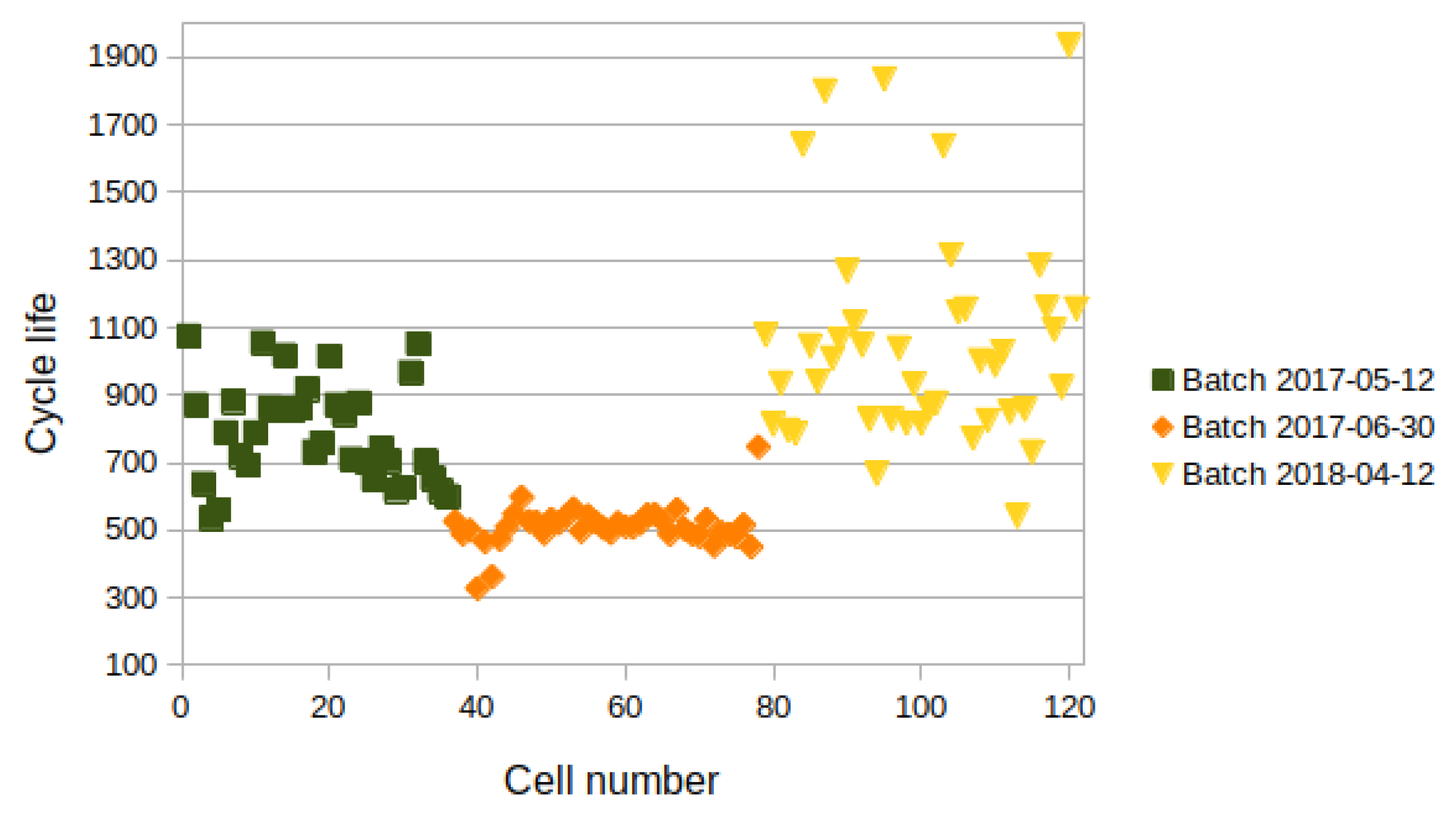
  • For batch “2017-05-12”, channels 1, 2, 3, 4, 5, 6, 8, 13, 19, 21, 22 and 31 were excluded. Channels 4 and 8 did not successfully start and thus did not have data. The cells in channels 1, 2, 3, 5 and 6 were stopped at the end of the test and resumed in the “2017-06-30” batch. This pause in cycling led to a rise in capacity upon resuming the tests. The tests in channels 13, 19, 21, 22 and 31 were terminated before the cells reached 80% of nominal capacity.
  • For batch “2017-06-30”, channels 1, 2, 3, 5, 6 and 10 were excluded. Channels 1, 2, 3, 5 and 6 were not new experiments but a continuation of experiments from the “2017-05-12” batch. The cell on channel 10 was possibly defective as it died quickly.
  • For batch “2018-04-12”, channels 26, 31, 33, 41 and 46 were excluded. No data were provided for channels 26 and 31. The tests in channels 33 and 41 were terminated before the cells reached 80% of the nominal capacity. The cell in channel 46 had noisy voltage profiles due to an electronic connection error.
Therefore, 121 channels were left in the analysis, where each channel represented one cell.
Some differences regarding the resting times were reported for each batch [6]. The cells in batch “2017-05-12” had two resting moments: one of 1 min after reaching the 80% state of charge (SoC) during charging and the other being 1 s after discharging. The cells in batch “2017-06-30” had two resting moments of 5 min each. The resting moments were also placed after reaching an 80% SoC during charging and after discharging. The cells in batch “2018-04-12”, as opposed to the previous batches, had four resting moments of 5 s each. The resting times were performed after reaching an 80% SoC during charging, after the internal resistance measurement, before discharging and after discharging. An additional difference between the batches was that the cells in batch “2017-06-30” were cycled until 75% of the nominal capacity, while the other two batches were cycled until 80% of the nominal capacity.
All the columns from the dataset were initially used in the prediction. However, more columns were created: variance of discharge capacity difference, variance of charge capacity difference and charging policies. As Severson et al. [6] stated, voltage curves are used to study battery characteristics and variance in probability theory, and their statistics could give better insight into the data. Therefore, it was expected that it would be relevant to include the variance of charge and discharge capacity in the analysis. This feature was first introduced by the authors and is explained with more details in the original publication [6]. In summary, it consists of calculating the difference in discharge capacities as a function of the voltage between cycle 10 and cycle 100. To create the additional columns for our research work, this feature was not only calculated for the discharge capacity but also for the charge capacity. The computation for the other input variable followed the same initial principal. A picture showing the difference in discharge capacity as a function of the voltage between cycle 10 and cycle 100 for an exemplary cell can be seen in Figure 1.
The charging policies data column was created by grouping all cells based on their most used C rates. The C rates of each cell can be found in the original publication [6]. Cells with C rates of 1, 2 or 3 were grouped as “high” C rates, cells with C rates of 4, 5 or 6 were grouped as “very high” C rates, and cells with C rates of 7 or 8 were grouped as “extremely high” C rates. These new columns were created as the charging rate greatly influences the degradation phenomena of the batteries [9,10,11].
First, a feedforward ANN with 11 layers was used to predict the cycle lives of the lithium-ion batteries. Data for the first 100 cycles for all 121 cells were used. The relation between the training and testing data was 75%/25%. The ANN parameters were optimized by using their learning curve responses. After optimization, one input layer, nine hidden layers and one output layer were chosen. Using the Adam optimizer, a learning rate of 0.001, 500 epochs and the mean absolute percentage error as a loss function were selected. By cross-validation and additional visual inspection of the loss curves, potential overfitting was minimized as much as possible given the limited size of the dataset. To measure the accuracy of the ANN, the metrics of the mean absolute error (MAE) and mean absolute percentage error (MAPE) were used, which are defined as
MAE = i = 1 n | Actual Predicted | n ,
MAPE   ( % ) = 100 1 n i = 1 n | Actual Predicted | Actual ,
where “Actual” and “Predicted” correspond to the measured and predicted cycle lives, respectively, and n is the total amount of samples.
The same code was applied to three sets of data: (1) the original raw data without any preprocessing; (2) the cycles that presented particularly noisy behavior or very high or low peaks, which were removed from the dataset; and (3) along with the noises, the first cycles of all cells were removed. Since the batteries were pre-charged, during the first cycle, they needed to initially discharge so that they could start cycling under controllable conditions later. This process of removing unwanted cycles is defined here as ”cleansing” the data.
Secondly, to investigate whether the ANN is the best ML approach to use, a fully automated algorithm called H2O AutoML [49] was applied. This algorithm compares, using the same dataset from the previous ANN analysis, the results from different ML methods and ranks all tested models by different performance metrics to find the best prediction. The algorithms that produced similar errors in comparison with the ANN were investigated in more detail. Their parameters were optimized. The relation between the training and testing data was kept at 75%/25%.
Thirdly, using the model that provided the best result thus far, the importance of the variables was investigated in order to eliminate unnecessary data columns and obtain a better physical understanding. Two variable importance analyses were carried out: Kendall’s tau and the Spearman coefficient [50,51]. In these analyses, scores close to zero indicate no relation between the input and the output values. On the other hand, scores approaching 1 or −1 indicate a strong relation between the input variables and output results. The sign denotes the direction of the correlation. A negative coefficient means that the variables are inversely related [52,53,54].
In the end, the errors obtained in this study were compared with other similar works found in the literature for the same dataset.

3. Results and Discussion

3.1. Prediction of Life Cycle

By following the procedures and using the datasets as described in the section above, the results for the MAE and MAPE of the ANN analysis are summarized in Table 1. The results show that removing noises, peaks and the first cycle did not improve the predictions from the control dataset. However, cleansing of the data improved the predictions for the dataset with the newly added input columns. The addition of the columns also generated better results. With the dataset amplified, errors smaller than 1% were obtained. The best result thus far was achieved by using the new dataset with additional input columns. Therefore, it can be said that at this point, the accuracy of the ANN was 99.43%.
The results corroborate the expectation that the additional columns and the removal of noises and first cycles should improve the results. These findings are in line with the reports from the literature, which show that the charging rate has an influence on the lifetime of the batteries [9,10,11].
Secondly, the algorithm H2O AutoML was used to compare different ML models. The dataset applied was the one that resulted in the best prediction in the previous ANN analysis (new dataset with additional columns). The MAE was the metric on which the comparison was based, and the results are depicted in Figure 2. The best models were DRF, XRT, and the GBM, with MAEs of 4.15 , 5.65 and 6.19 cycles, respectively. The best ANN analysis produced an MAE of 4.65 cycles. Meanwhile, DL and the GLM returned errors substantially higher than the ANN reference value. An additional advantage of these algorithms is that they are significantly more agile than ANNs. The ANN model performed training and prediction in approximately 15 min, while the new methods took only seconds.
The three best models were investigated in more detail, and their parameters were optimized. The detailed results for these models are shown in Table 2. It can be observed that the smallest error was obtained using the XRT model, which gave a prediction accuracy of 99.81%.
To put it succinctly, adding hand-featured inputs to the raw data clearly improved the prediction of the cells’ lifetimes. Cleaning the data of noises and peaks and removing the first cycles generated better results, mainly for the dataset in which these new input data were included. For the same dataset, six different ML models were compared, namely the ANN, DRF, XRT, GBM, DL and GLM. From these, the best predictions were obtained via XRT, which output an MAPE of only 0.19%.

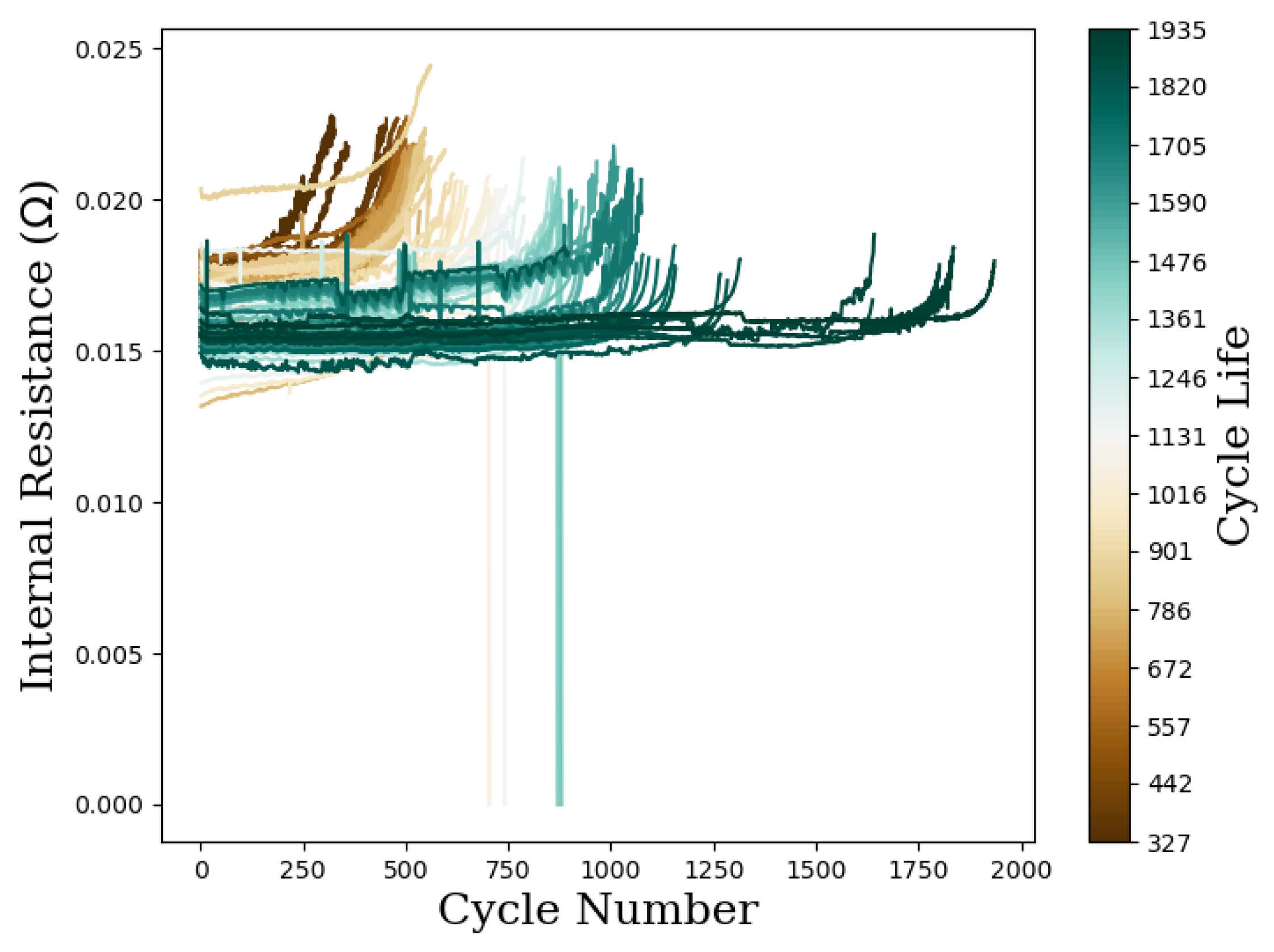
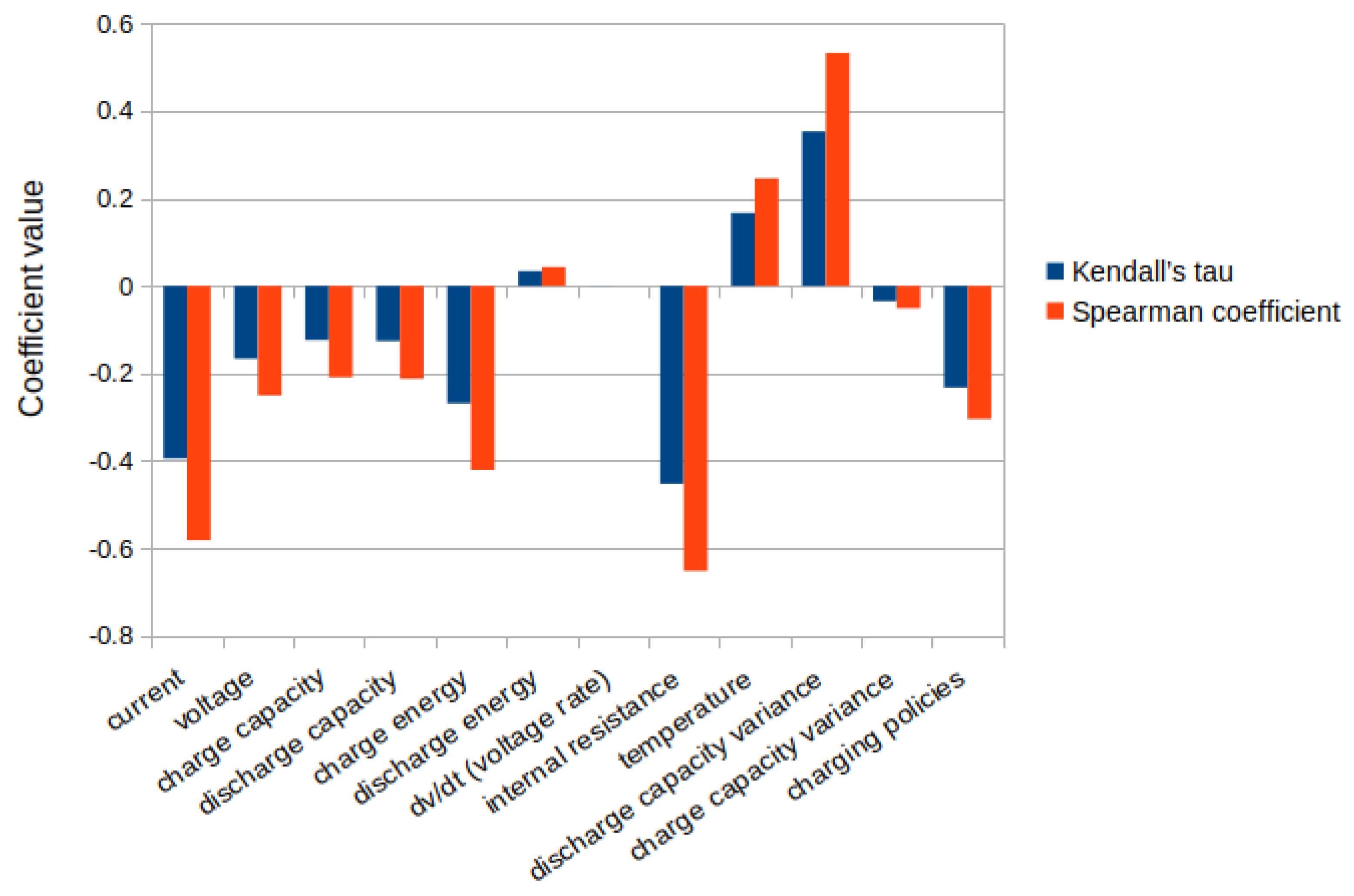
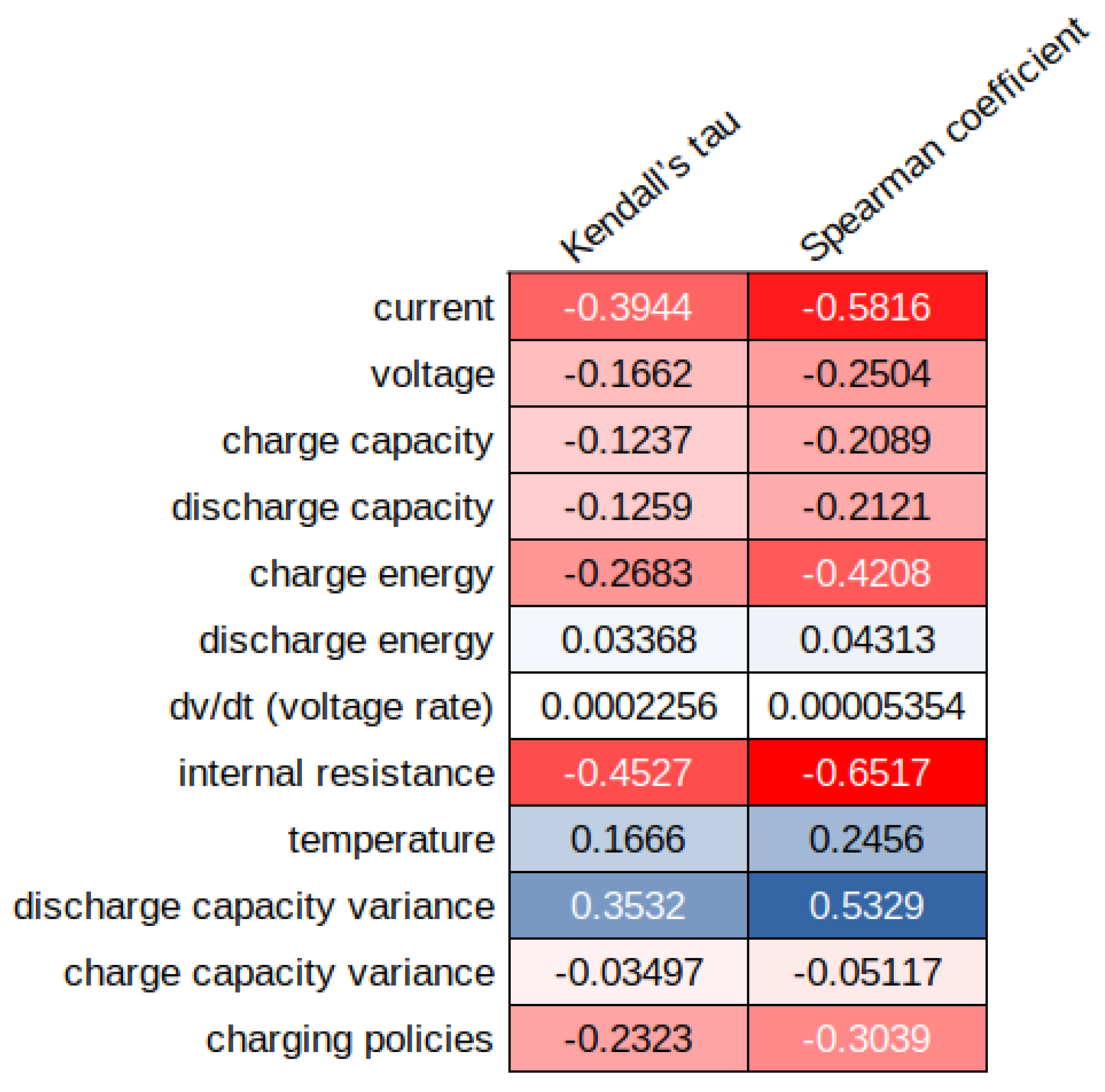
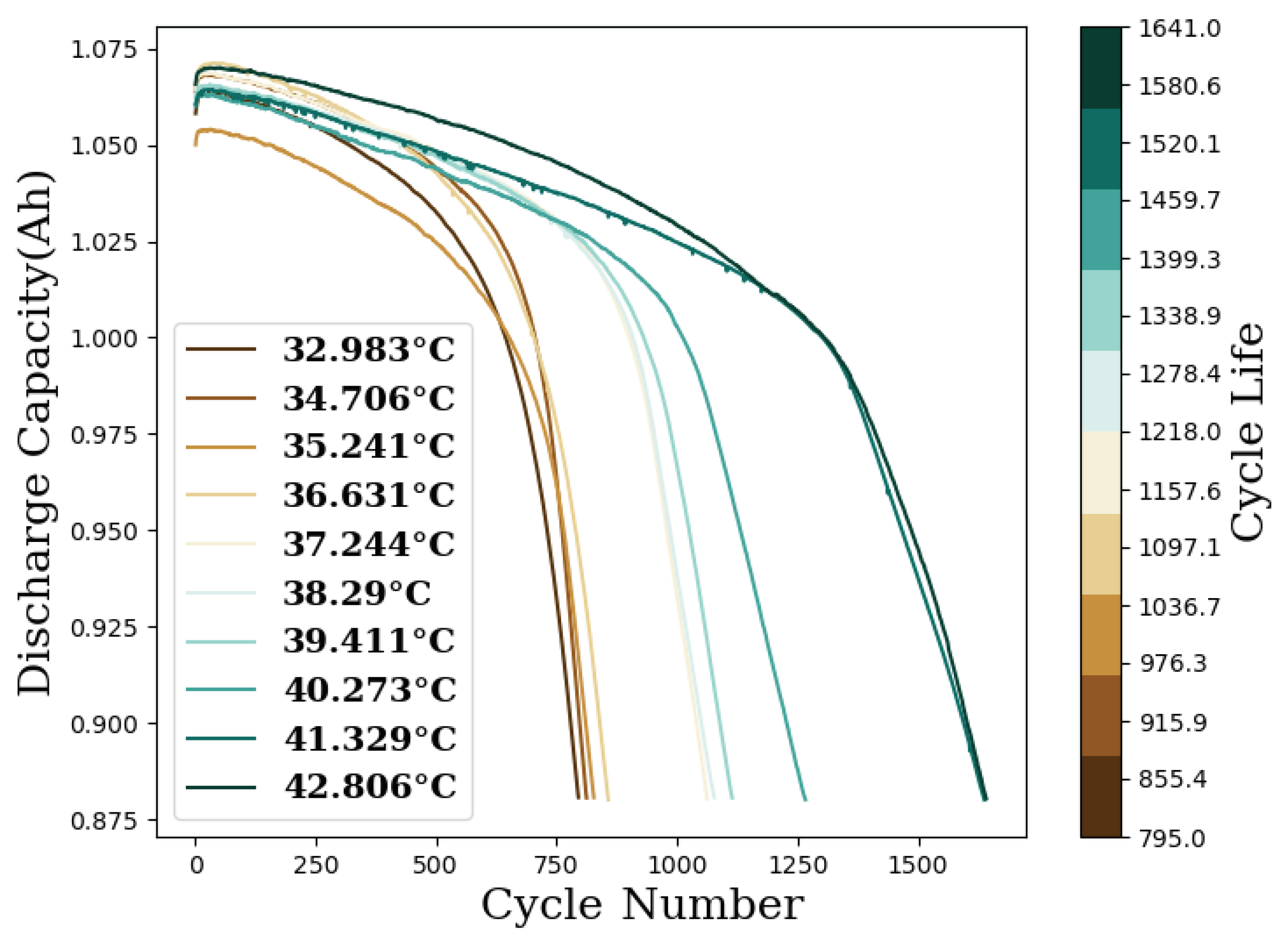
3.2. Analysis of Input Variables

The cycle lives of all analyzed cells are depicted in Figure 3. There were different distributions of lifetimes for the three batches, where the highest lifetimes belonged to batch “2018-04-12” and the shortest to batch “2017-06-30”. The batches differed in the resting times while cycling, as described in the Section 2. One observation that can be made is that the cells with the shortest cycle lives belonged to the batch with the longer resting times. Longer relaxation times have already been linked to higher impedance measurements in experiments [55]. A similar correlation seemed to happen in the data from Severson et al. [6].
Additionally, the discharge capacities of the analyzed cells can be seen in Figure 4 as well as the internal resistance in Figure 5. The color set-up indicates the lifetimes of the cells. Cells with higher initial internal resistance ended up with shorter lifetimes. These were mostly the cells belonging to the batch “2017-06-30”, which was the batch with longer resting times. Another observation is that those cells from batch “2017-06-30” were cycled until reaching 75% nominal capacity, while the remaining two batches were cycled until 80% nominal capacity. Therefore, the cells were easy to spot when the discharge capacity was plotted, as their curves were slightly longer.
To better analyze the input features, the importance of the variables for the XRT model was investigated using two different models: Kendall’s tau and the Spearman coefficient. The results are shown in Figure 6 and Figure 7. A score which tends toward zero indicates that no correlation is present. Meanwhile, a score tending toward 1 or −1 indicates a strong correlation between the input variables and the cycle life. The sign denotes the direction of the correlation. A negative coefficient means that the variables are inversely related [52]. In this analysis, it can be seen that the discharge energy, voltage rate and charge capacity variance were the features with the smallest importance coefficients, meaning that they were the least important ones. On the other hand, the features of the current, internal resistance and discharge capacity variance appeared to be the most relevant ones.
Features such as the discharge energy, charge energy, discharge capacity and charge capacity showed poor correlation with the cycle life. A trivial link between the discharge capacity and cycle life existed, as the curves show a slower degradation for higher lifetimes. Nevertheless, for the first 100 cycles, this weak relationship between the initial capacity and lifetime has already been pointed out [6]. On the other hand, the discharge capacity variance had a strong connection with the lifetime. This fact has already been explored as well [6].
The current and the charging policies had a strong negative correlation with the cycle life, meaning that when these two variables increased in value, the cycle life decreased. This agrees with previous publications, which showed that some of the most relevant stress factors for the degradation of batteries are exposure to high currents and high charging rates [9,10,11,12,13]. It was also already anticipated that the internal resistance would rank in between the most important variables, since the increase in internal resistance is deeply connected to the decrease in battery capacity [14]. Contrarily, the voltage rate appeared to have a zero score, indicating no relation with the cycle life. Neglecting this quantity reduced computational demand and the complexity of the XRT model. Thus, when the voltage rate was removed from the analysis, the prediction errors remained the same, and the dataset could be reduced without deteriorating the predictions. If more columns were removed, the results were worsened.
The measured temperatures of the cells showed a weak relation with the cycle life. However, it has been observed that cells with short lifetimes have lower final temperatures than cells with long cycle lives. This relation can be seen in Figure 8. It can be suggested that this is simply due to heating up the cells during operation. Nonetheless, the literature indicates that higher temperatures induce lower impedance measurements [55]. It must be noted that the temperature measurements are not perfectly reliable, as the thermal contact between the thermocouple and the cell may vary substantially, with contact sometimes even being lost in the course of the experiment [6].
It becomes clear that the variable importance analysis can correlate with physics and support detecting the possible factors influencing the degradation of batteries. The current, internal resistance, discharge capacity variance and charging policies appeared to be highly important input variables. Aside form that, the data also suggest that the resting times have an influence on internal resistance and, consequently, on the cycle life. Nevertheless, this point requires further research to be fully confirmed.

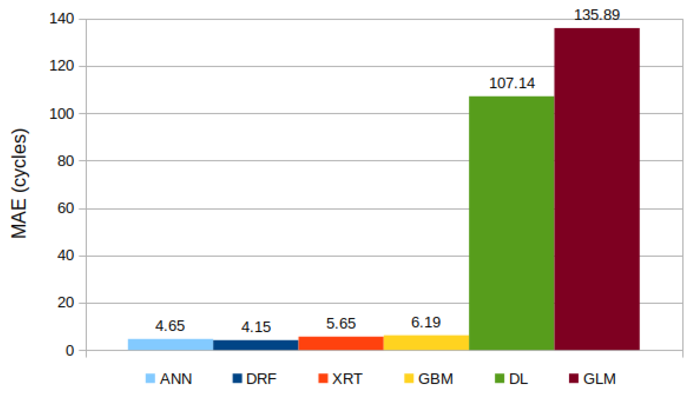
3.3. Prediction Error Comparison

Using the same dataset, Severson et al. [6] obtained an error of 9.1% using an elastic net model. Since then, a number of studies have applied their published raw data in self-developed ML models. Research groups have used different ML methods, input parameters and cycle numbers. A summary of some main works, including the current study, can be seen in Table 3. It becomes clear that the errors published in the literature are significantly larger than the ones acquired in our study. We believe that the smaller error can be attributed to assembling physical understanding, optimizing the ML models and manipulating the data. By understanding the data, cleansing it, adding additional inputs and optimizing the ML models, the results were substantially improved.

4. Conclusions

In this study, the cycle life of commercial lithium-ion batteries was successfully predicted using only early-cycle literature-available data and ML algorithms. The degradation phenomena of such batteries are complex, rely on many factors and follow a nonlinear trajectory. In this context, the use of data-driven models, which are in principal agnostic to chemistry, is compelling. The disadvantages of such models are access to reliable data and extraction of physical understanding. To tackle these issues, literature data were used, and the data were managed in order to generate physical insights. The cells which presented unusual behavior were excluded, new features were calculated and added to the prediction, and the importance of the input variables was investigated.
The results show that the prediction performed by the ANN was extremely accurate (99.43% accuracy) when removal of defectuous cells, noises and spikes and the addition of information about charging protocols and capacity variances were performed. The accuracy was further improved when a superior ML algorithm (XRT) was chosen, reaching 99.81%. XRT, also presenting a significantly faster running time. The computational time was reduced from 15 min with the ANN to less than a second with XRT. The errors obtained in our study were substantially lower than what was found in comparable works in the current literature. More generally, this example shows that the comparative use of different machine learning algorithms, as supported, for example, by the H 2 O AutoML library, can be beneficial and is therefore also recommended for other applications.
Lastly, the variables’ importance results provided information about the relevance of experimental inputs regarding the degradation phenomena. A feature such as the voltage rate ranked as the least important and could be removed from the analysis without deteriorating the accuracy. On the other hand, features such as the internal resistance, current, discharge capacity variance and charging policies ranked as the most important ones and were very relevant for the developed model. Aside from that, the data suggest that long resting times should be avoided to achieve a long cycle life.
Whereas the present analysis emerges as a successful method to predict the battery lifetime for the given dataset, the transfer toward other cell chemistries would require retraining or at least an adjustment of the model’s parameters. We believe that coupling it with detailed chemo-physical models would allow even further optimizations and lead to more robust predictions. An additional valuable future goal will be to adapt the model to be applied to in situ data such as, for example, those obtained throughout the drive cycles of electrical vehicles.

Author Contributions

Conceptualization, R.S. (Robert Spatschek) and B.C.; methodology, software and validation, B.C.; formal analysis, investigation, visualization and writing, B.C., R.S. (Roland Sandt) and L.C.P.d.S.; supervision, project administration and funding acquisition, R.S. (Robert Spatschek). All authors have read and agreed to the published version of the manuscript.

Funding

This research was funded by the German Federal Ministry of Education and Research (BMBF) via the project Meet HiEnD 3 and the Helmholtz project ZeDaBase. Open access was funded by the Deutsche Forschungsgemeinschaft (DFG, German Research Foundation)—491111487.

Data Availability Statement

Not applicable.

Acknowledgments

The authors gratefully acknowledge the computing time granted by the JARA Vergabegremium and provided on the JARA Partition part of the supercomputer JURECA at Forschungszentrum Jülich [56].

Conflicts of Interest

The authors declare no conflict of interest.

Abbreviations

The following abbreviations are used in this manuscript:
SEISolid electrolyte interphase
MLMachine learning
ANNArtificial neural network
DRFDefault random forest
GBMGradient boosting models
XRTExtremely randomized trees
DLDeep learning
GLMGeneralized linear model
NASANational Aeronautics and Space Administration
NRELNational Renewable Energy Laboratory
SoCState of charge
MAEMean absolute error
MAPEMean absolute percentage error

References

  1. Grey, C.; Hall, D. Prospects for lithium-ion batteries and beyond—A 2030 vision. Nat. Commun. 2020, 11, 2–5. [Google Scholar] [CrossRef] [PubMed]
  2. Wen, J.; Yu, Y.; Chen, C. A review on lithium-ion batteries safety issues: Existing problems and possible solutions. Mater. Express 2012, 2, 197–212. [Google Scholar] [CrossRef]
  3. Han, X.; Lu, L.; Zheng, Y.; Feng, X.; Li, Z.; Li, J.; Ouyang, M. A review on the key issues of the lithium ion battery degradation among the whole life cycle. eTransportation 2019, 1, 100005. [Google Scholar] [CrossRef]
  4. Barré, A.; Deguilhem, B.; Grolleau, S.; Gérard, M.; Suard, F.; Riu, D. A review on lithium-ion battery ageing mechanisms and estimations for automotive applications. J. Power Sources 2013, 241, 680–689. [Google Scholar] [CrossRef] [Green Version]
  5. Vetter, J.; Novák, P.; Wagner, M.; Veit, C.; Möller, K.C.; Besenhard, J.; Winter, M.; Wohlfahrt-Mehrens, M.; Vogler, C.; Hammouche, A. Ageing mechanisms in lithium-ion batteries. J. Power Sources 2005, 147, 269–281. [Google Scholar] [CrossRef]
  6. Severson, K.; Attia, P.; Jin, N.; Perkins, N.; Jiang, B.; Yang, Z.; Chen, M.; Aykol, M.; Herring, P.; Fraggedakis, D.; et al. Data-driven prediction of battery cycle life before capacity degradation. Nat. Energy 2019, 4, 383–391. [Google Scholar] [CrossRef] [Green Version]
  7. Wang, A.; Kadam, S.; Li, H.; Shi, S.; Qi, Y. Review on modeling of the anode solid electrolyte interphase (SEI) for lithium-ion batteries. NPJ Comput. Mater. 2018, 4, 15. [Google Scholar] [CrossRef] [Green Version]
  8. Nie, M.; Abraham, D.; Chen, Y.; Bose, A.; Lucht, B. Silicon solid electrolyte interphase (SEI) of lithium battery characterized by microscopy and spectroscopy. J. Phys. Chem. C 2013, 117, 13403–13412. [Google Scholar] [CrossRef]
  9. An, S.; Li, J.; Daniel, C.; Mohanty, D.; Nagpure, S.; Wood, D. The state of understanding of the lithium-ion-battery graphite solid electrolyte interphase (SEI) and its relationship to formation cycling. Carbon 2016, 105, 52–76. [Google Scholar] [CrossRef] [Green Version]
  10. Li, Y.; Liu, K.; Foley, A.; Zülke, A.; Berecibar, M.; Nanini-Maury, E.; Van Mierlo, J.; Hoster, H. Data-driven health estimation and lifetime prediction of lithium-ion batteries: A review. Renew. Sustain. Energy Rev. 2019, 113, 109254. [Google Scholar] [CrossRef]
  11. Keil, P.; Jossen, A. Charging protocols for lithium-ion batteries and their impact on cycle life - An experimental study with different 18650 high-power cells. J. Energy Storage 2016, 6, 125–141. [Google Scholar] [CrossRef]
  12. Leng, F.; Tan, C.; Pecht, M. Effect of Temperature on the Aging rate of Li Ion Battery Operating above Room Temperature. Sci. Rep. 2015, 5, 12967. [Google Scholar] [CrossRef] [PubMed] [Green Version]
  13. Pinson, M.; Bazant, M. Theory of SEI Formation in Rechargeable Batteries: Capacity Fade, Accelerated Aging and Lifetime Prediction. J. Electrochem. Soc. 2013, 160, A243–A250. [Google Scholar] [CrossRef]
  14. Schuster, S.; Bach, T.; Fleder, E.; Müller, J.; Brand, M.; Sextl, G.; Jossen, A. Nonlinear aging characteristics of lithium-ion cells under different operational conditions. J. Energy Storage 2015, 1, 44–53. [Google Scholar] [CrossRef]
  15. Krewer, U.; Röder, F.; Harinath, E.; Braatz, R.; Bedürftig, B.; Findeisen, R. Review—Dynamic Models of Li-Ion Batteries for Diagnosis and Operation: A Review and Perspective. J. Electrochem. Soc. 2018, 165, A3656–A3673. [Google Scholar] [CrossRef]
  16. Chen, C.; Zuo, Y.; Ye, W.; Li, X.; Deng, Z.; Ong, S. A Critical Review of Machine Learning of Energy Materials. Adv. Energy Mater. 2020, 10, 1903242. [Google Scholar] [CrossRef]
  17. Ng, M.F.; Zhao, J.; Yan, Q.; Conduit, G.; Seh, Z. Predicting the state of charge and health of batteries using data-driven machine learning. Nat. Mach. Intell. 2020, 2, 161–170. [Google Scholar] [CrossRef] [Green Version]
  18. Waag, W.; Fleischer, C.; Sauer, D. Critical review of the methods for monitoring of lithium-ion batteries in electric and hybrid vehicles. J. Power Sources 2014, 258, 321–339. [Google Scholar] [CrossRef]
  19. Si, X.; Wang, W.; Hu, C.; Zhou, D. Remaining useful life estimation—A review on the statistical data driven approaches. Eur. J. Oper. Res. 2011, 213, 1–14. [Google Scholar] [CrossRef]
  20. Abiodun, O.; Jantan, A.; Omolara, A.; Dada, K.; Mohamed, N.; Arshad, H. State-of-the-art in artificial neural network applications: A survey. Heliyon 2018, 4, e00938. [Google Scholar] [CrossRef]
  21. Yang, D.; Wang, Y.; Pan, R.; Chen, R.; Chen, Z. A Neural Network Based State-of-Health Estimation of Lithium-ion Battery in Electric Vehicles. Energy Procedia 2017, 105, 2059–2064. [Google Scholar] [CrossRef]
  22. You, G.w.; Park, S.; Oh, D. Real-time state-of-health estimation for electric vehicle batteries: A data-driven approach. Appl. Energy 2016, 176, 92–103. [Google Scholar] [CrossRef]
  23. Guo, Y.; Zhao, Z.; Huang, L. SoC Estimation of Lithium Battery Based on Improved BP Neural Network. Energy Procedia 2017, 105, 4153–4158. [Google Scholar] [CrossRef]
  24. Biau, G.; Scornet, E. A random forest guided tour. Test 2016, 25, 197–227. [Google Scholar] [CrossRef] [Green Version]
  25. Natekin, A.; Knoll, A. Gradient boosting machines, a tutorial. Front. Neurorobot. 2013, 7, 21. [Google Scholar] [CrossRef] [PubMed] [Green Version]
  26. Geurts, P.; Ernst, D.; Wehenkel, L. Extremely randomized trees. Mach. Learn. 2006, 63, 3–42. [Google Scholar] [CrossRef] [Green Version]
  27. Lecun, Y.; Bengio, Y.; Hinton, G. Deep learning. Nature 2015, 521, 436–444. [Google Scholar] [CrossRef]
  28. Dobson, A.; Barnett, A. An Introduction to Generalized Linear Models, 4th ed.; Chapman and Hall/CRC: Boca Raton, FL, USA, 2018; p. 392. [Google Scholar] [CrossRef]
  29. Andersson, S.; Bathula, D.; Iliadis, S.; Walter, M.; Skalkidou, A. Predicting women with depressive symptoms postpartum with machine learning methods. Sci. Rep. 2021, 11, 7877. [Google Scholar] [CrossRef]
  30. Finegan, D.; Zhu, J.; Feng, X.; Keyser, M.; Ulmefors, M.; Li, W.; Bazant, M.; Cooper, S. The Application of Data-Driven Methods and Physics-Based Learning for Improving Battery Safety. Joule 2021, 5, 316–329. [Google Scholar] [CrossRef]
  31. Finegan, D.; Cooper, S. Battery Safety: Data-Driven Prediction of Failure. Joule 2019, 3, 2599–2601. [Google Scholar] [CrossRef]
  32. Attia, P.; Grover, A.; Jin, N.; Severson, K.; Markov, T.; Liao, Y.; Chen, M.; Cheong, B.; Perkins, N.; Yang, Z.; et al. Closed-loop optimization of fast-charging protocols for batteries with machine learning. Nature 2020, 578, 397–402. [Google Scholar] [CrossRef] [PubMed] [Green Version]
  33. Li, W.; Zhu, J.; Xia, Y.; Gorji, M.; Wierzbicki, T. Data-Driven Safety Envelope of Lithium-Ion Batteries for Electric Vehicles. Joule 2019, 3, 2703–2715. [Google Scholar] [CrossRef]
  34. Johnen, M.; Pitzen, S.; Kamps, U.; Kateri, M.; Dechent, P.; Sauer, D. Modeling long-term capacity degradation of lithium-ion batteries. J. Energy Storage 2021, 34, 102011. [Google Scholar] [CrossRef]
  35. Walker, W.; Darst, J.; Finegan, D.; Bayles, G.; Johnson, K.; Darcy, E.; Rickman, S. Decoupling of heat generated from ejected and non-ejected contents of 18650-format lithium-ion cells using statistical methods. J. Power Sources 2019, 415, 207–218. [Google Scholar] [CrossRef]
  36. Finegan, D.; Darst, J.; Walker, W.; Li, Q.; Yang, C.; Jervis, R.; Heenan, T.; Hack, J.; Thomas, J.; Rack, A.; et al. Modelling and experiments to identify high-risk failure scenarios for testing the safety of lithium-ion cells. J. Power Sources 2019, 417, 29–41. [Google Scholar] [CrossRef]
  37. Yin, A.; Tan, Z.; Tan, J. Life prediction of battery using a neural gaussian process with early discharge characteristics. Sensors 2021, 21, 1087. [Google Scholar] [CrossRef] [PubMed]
  38. Fei, Z.; Zhang, Z.; Yang, F.; Tsui, K.; Li, L. Early-stage lifetime prediction for lithium-ion batteries: A deep learning framework jointly considering machine-learned and handcrafted data features. J. Energy Storage 2022, 52, 104936. [Google Scholar] [CrossRef]
  39. Strange, C.; dos Reis, G. Prediction of future capacity and internal resistance of Li-ion cells from one cycle of input data. Energy AI 2021, 5, 100097. [Google Scholar] [CrossRef]
  40. Hsu, C.; Xiong, R.; Chen, N.; Li, J.; Tsou, N. Deep neural network battery life and voltage prediction by using data of one cycle only. Appl. Energy 2022, 306, 118134. [Google Scholar] [CrossRef]
  41. Alipour, M.; Tavallaey, S.; Andersson, A.; Brandell, D. Improved Battery Cycle Life Prediction Using a Hybrid Data-Driven Model Incorporating Linear Support Vector Regression and Gaussian. ChemPhysChem 2022, 23, e202100829. [Google Scholar] [CrossRef]
  42. Gong, D.; Gao, Y.; Kou, Y.; Wang, Y. Early prediction of cycle life for lithium-ion batteries based on evolutionary computation and machine learning. J. Energy Storage 2022, 51, 104376. [Google Scholar] [CrossRef]
  43. Afshari, S.; Cui, S.; Xu, X.; Liang, X. Remaining Useful Life Early Prediction of Batteries Based on the Differential Voltage and Differential Capacity Curves. IEEE Trans. Instrum. Meas. 2022, 71, 3117631. [Google Scholar] [CrossRef]
  44. Zhang, Y.; Peng, Z.; Guan, Y.; Wu, L. Prognostics of battery cycle life in the early-cycle stage based on hybrid model. Energy 2021, 221, 119901. [Google Scholar] [CrossRef]
  45. Yang, F.; Wang, D.; Xu, F.; Huang, Z.; Tsui, K. Lifespan prediction of lithium-ion batteries based on various extracted features and gradient boosting regression tree model. J. Power Sources 2020, 476, 228654. [Google Scholar] [CrossRef]
  46. Fei, Z.; Yang, F.; Tsui, K.; Li, L.; Zhang, Z. Early prediction of battery lifetime via a machine learning based framework. Energy 2021, 225, 120205. [Google Scholar] [CrossRef]
  47. Brandt, N.; Griem, L.; Herrmann, C.; Schoof, E.; Tosato, G.; Zhao, Y.; Zschumme, P.; Selzer, M. Kadi4Mat: A Research Data Infrastructure for Materials Science. Data Sci. J. 2021, 20, 8. [Google Scholar] [CrossRef]
  48. Stonebraker, M.; Rowe, L. The design of POSTGRES. ACM SIGMOD Record 1986, 15, 340–355. [Google Scholar] [CrossRef]
  49. LeDell, E.; Poirier, S. H2O AutoML: Scalable Automatic Machine Learning. In Proceedings of the 7th ICML Workshop on Automated Machine Learning (AutoML), Online, 18 July 2020. [Google Scholar]
  50. Kendall, M.G. A new measure of rank correlation. Biometrika 1938, 30, 81–93. [Google Scholar] [CrossRef]
  51. Spearman, C. The Proof and Measurement of Association between Two Things. Am. J. Psychol. 1904, 15, 72–101. [Google Scholar] [CrossRef]
  52. Akoglu, H. User’s guide to correlation coefficients. Turk. J. Emerg. Med. 2018, 18, 91–93. [Google Scholar] [CrossRef]
  53. Pedregosa, F.; Varoquaux, G.; Gramfort, A.; Michel, V.; Thirion, B.; Grisel, O.; Blondel, M.; Prettenhofer, P.; Weiss, R.; Dubourg, V.; et al. Scikit-learn: Machine Learning in Python. J. Mach. Learn. Res. 2011, 12, 2825–2830. [Google Scholar]
  54. Buitinck, L.; Louppe, G.; Blondel, M.; Pedregosa, F.; Mueller, A.; Grisel, O.; Niculae, V.; Prettenhofer, P.; Gramfort, A.; Grobler, J.; et al. API design for machine learning software: Experiences from the scikit-learn project. In Proceedings of the ECML PKDD Workshop: Languages for Data Mining and Machine, Prague, Czech Republic, 23–27 September 2013. [Google Scholar]
  55. Keil, P. Aging of Lithium-Ion Batteries in Electric Vehicles. Ph.D. Thesis, Technische Universität München, München, Germany, 2017. [Google Scholar]
  56. Jülich Supercomputing Centre. JURECA: Data Centric and Booster Modules implementing the Modular Supercomputing Architecture at Jülich Supercomputing Centre. J. Large-Scale Res. Facil. 2018, 7, A182. [Google Scholar] [CrossRef]
Figure 1. Difference in discharge capacity as a function of voltage between cycle 10 and cycle 100 for an exemplary cell.
Batteries 08 00266 g001
Figure 2. Results for mean absolute error (MAE) from different ML algorithms obtained via H 2 O AutoML.
Batteries 08 00266 g002
Figure 3. Resulting distribution of cycle lives of all analyzed cells. The different colors correspond to each experimental batch. One difference between the three batches is the resting times while cycling. The cells with the shortest cycle lives belonged to batch “2017-06-30”, which was the batch with the longer resting times.
Batteries 08 00266 g003
Figure 4. Discharge capacity versus cycle number of all analyzed cells. The different colors indicate the corresponding cycle life of each cell. The cells with shorter lives belonged to batch “2017-06-30”, which was cycled until 75% nominal capacity. The remaining two batches were cycled until 80% nominal capacity.
Batteries 08 00266 g004
Figure 5. Internal resistance of all analyzed cells. The different colors indicate the corresponding cell cycle life. The higher the internal resistance, the shorter the lifetime. The cells with the shortest lifetimes belonged to batch “2017-06-30”, which was the batch with longer resting times. The batches differed regarding the resting times.
Batteries 08 00266 g005
Figure 6. Results from variable importance analysis. Kendall’s tau and Spearman coefficient for all input features were evaluated. Values close to 0 mean no importance, while values close to either 1 or −1 mean strong correlation.
Batteries 08 00266 g006
Figure 7. Results from variable importance analysis. Kendall’s tau and Spearman coefficient for all input features were evaluated. Values close to 0 (white color) mean no importance, while values close to either 1 (blue color) or −1 (red color) mean strong correlation.
Batteries 08 00266 g007
Figure 8. Discharge capacities of exemplary cells for different final testing temperatures. All cells started cycling with similar temperatures, but cells with longer cycle lives presented higher final testing temperatures.
Batteries 08 00266 g008
Table 1. Results for mean absolute error (MAE) and mean absolute percentage error (MAPE) from the ANN algorithm (1st: with raw data; 2nd: removing noise and peaks; 3rd: removing noise, peaks and the first cycle). The control dataset was compared against the dataset with newly added input features.
Dataset1st: MAE (Cycles)/MAPE (%)2nd: MAE (Cycles)/MAPE (%)3rd: MAE (Cycles)/MAPE (%)
Control12.16/1.5413.00/1.7113.81/1.68
New7.78/0.887.06/0.874.65/0.57
Table 2. Results for mean absolute error (MAE) and mean percentage error (MAPE) from default random forest (DRF), extremely randomized trees (XRT) and gradient boosting models (GBMs). The corresponding parameters were optimized.
ModelMAE (Cycles)MAPE (%)
XRT1.490.19
DRF2.150.30
GBM3.610.49
Table 3. Results for current work and comparable literature studies using the same dataset.
Ref.Number of Cells Analyzed from the DatabaseNumber of Input CyclesML MethodLowest MAPE (%)
This work121100Extremely randomized trees0.19
[6]124100Elastic net9.1
[37]124110Neural Gaussian process8.8
[38]123100Gaussian process regression8.2
[39]124100Convolutional neural networks8.6
[40]95100Deep neural network3.97
[41]Less than 124 *100Linear support vector regression and Gaussian process regression8.2
[42]123100Elastic net5.21
[43]124100Bayesian sparse learning8.4
[44]12380Random forest, artificial bee colony and general regression neural network6.3
[45]124250Gradient boosting regression tree7.0
[46]124100Support vector machine8.0
* The authors mentioned that some cells were removed from the analysis, but they did not specify the quantity.
Publisher’s Note: MDPI stays neutral with regard to jurisdictional claims in published maps and institutional affiliations.

