Deploying Virtual Quality Gates in a Pilot-Scale Lithium-Ion Battery Assembly Line

Abstract

Pilot production is a critical transitional phase in the process of new product development or manufacturing, aiming at ensuring that products are thoroughly validated and optimized before entering full-scale production. During this stage, a key challenge is how to leverage limited resources to build data infrastructure and conduct data analysis to establish and verify quality control. This paper presents the implementation of a cyber–physical system (CPS) for a lithium battery pilot assembly line. A machine learning-based predictive model was employed to establish quality control mechanisms. Process knowledge-guided data analysis was utilized to build a quality prediction model based on the collected battery data. The model-centric concept of ‘virtual quality’ enables early quality judgment during production, which allows for flexible quality control and the determination of optimal process parameters, thereby reducing production costs and minimizing energy consumption during manufacturing.

1. Introduction

The pilot production phase refers to the small-scale trial production conducted before entering full-scale manufacturing [1]. During this stage, aspects such as product design, manufacturing technique, equipment configuration, process parameters, and quality control measurements are validated and adjusted within a practical production environment [2]. The increasingly fierce market competition demands that manufacturing companies swiftly adapt to new technologies, new processing materials, and material or energy cost fluctuations. This imposes higher requirements on pilot production. To stay competitive, companies need to conduct pilot production efficiently while thoroughly investigating the interrelationships between quality parameters and process parameters during manufacturing. This is essential for determining the optimal process parameters and establishing a quality control system for mass production. Data-driven quality analysis offers solutions for handling such a challenge.

Once the product design, manufacturing techniques, and manufacturing equipment have been established, another critical objective during pilot production is to identify the quality-related process parameters. For each quality indicator, acceptable tolerance ranges must be defined according to the specified quality requirements and standards. Various studies have introduced quality assurance methods for individual processes within battery production. For example, defect analysis of electrode coatings, optical inspection of electrode surface particles using optical camera systems after pre-treatment, and online detection systems for separator manufacturing have been extensively documented [3,4]. However, these quality assurance schemes targeting single processes do not automatically constitute a comprehensive quality management system that ensures overall product quality.

Due to the complexity of the LIB production chain, traditional quality management tools such as Statistical Process Control (SPC) and Process Capability Indices quickly encounter limitations when applied [5]. Thus, the concept of Quality Gates (QGs) has been introduced to address the challenges posed by complex interrelationships [6]. The core idea of this concept is to systematically divide the defined manufacturing chain into different quality-related decision points. At these QGs, the intermediate quality of the product or the predicted final quality indicators are inspected to ensure that the required quality attributes have been met before proceeding to a further manufacturing step [7]. To construct a valid machine learning (ML) model capable of predicting the quality characteristics of a product, readily available data from the production environment can be utilized. This forms the foundation for advanced quality management, enabling both quality enhancement and high process transparency at minimal cost. The maturity of digitalization solutions enables the timely aggregation and processing of process information during production, allowing decision-making related to quality control to be implemented in a data-driven manner [8].

Unlike data analyses that focus on pursuing high-accuracy predictions, data-driven quality analysis emphasizes the development of transparent and interpretable ML models. In this context, approaches such as ‘explainable ML’, ‘informed ML’, and similar methodologies have been widely discussed [9]. Not all algorithms are inherently interpretable. In this article, we follow the terminology set by [10] and adopt the term ‘interpretable’ for all forms of explainable ML models. One direction addresses informed ML, which includes domain-specific knowledge as constraints in the ML optimization loop. One example is physic-informed or physic-constrained ML [11], which allows us to ensure physical consistency for model results [12]. Interpretable ML models have been applied, for instance, in healthcare [13], process engineering, e.g., biomethane production [14], or lithium-ion battery (LIB) manufacturing [15]. In process engineering, the lack of interpretability can greatly exacerbate the difficulty of conducting comprehensive and in-depth process analyses and may challenge the reliability of data-driven predictions. These issues are magnified in the context of small data volumes, where data resources available for analysis are limited [16].

The use of ML for data analysis is, nevertheless, necessary in small-data contexts, especially when conventional data analysis methods are failing in multidimensional parameter spaces. In the pilot production phase, data analysis is often constrained by the lack of data resources. Even when available data volumes are abundant, cost-effective data analysis is necessary to reduce the total investment. Domain-specific feature engineering can be applied to address the challenges associated with limited data: Dawson-Elli et al. illustrate how the use of physically meaningful features leads to improved model accuracy [17]. Such feature selection allows for dimensionality reduction and contributes to the efficient utilization of limited data resources. It also enhances plausibility checks, as features can be designed to relate to meaningful quantities.

This paper presents the implementation of a cyber–physical system (CPS) for a lithium battery pilot assembly line. A machine learning (ML) based predictive model was employed to establish quality control mechanisms. The paper is structured as follows. Section 2 provides a brief overview of the assembly line for LIBs established in the laboratory. This assembly line is used as a case study to introduce the establishment and components of a quality evaluation system based on the concept of virtual quality gates. The deployment of this virtual quality gate system, along with the actual data obtained during the project, is illustrated in Section 3. Section 4 summarizes the contribution of this paper.

2. Virtual Quality Gate for LIB Cell Assembly

This section focuses on LIB cell production with an emphasis on cell assembly. It outlines the procedure for establishing a quality control system based on quality gates for a pilot production line.

2.1. LIB Cell Production

The production of lithium-ion battery cells involves three main process steps: electrode manufacturing, cell assembly, and cell finishing. In this article, the cell assembly and the cell finishing are focused. Depending on the cell type, the cell assembly line may contain different manufacturing steps and machining methods. An assembly line for pouch cells in our laboratory is shown in Figure 1. It also indicates the sensors integrated into the production line for the monitoring of process parameters. The data collected by these sensors are transmitted to a unified data space. This ontology-based data space serves as one of the foundations for data-driven process analysis. Start with the roll material sheets; a separation step is carried out with a pouching tool. The components of a pouch, the anode and the cathode, are separated into individual groups. To control the rest of the moisture, the anodes and cathodes are dried in a post-drying step. Note that the post-drying is relative to the first drying after coating in electrode manufacturing. After the post-drying step, cell production requires a controlled atmosphere. This is usually achieved in a laboratory-scale production line with a glove box. As depicted in the figure, multiple anodes and cathodes are stacked into the Z-folded separator in the glove box during the stacking step. In a subsequent process, this stack is encapsulated and filled with electrolytes. In the cell finishing stage, the cell is activated by the first charge and discharge procedure. The gas generated during formation is removed, and the cell is finally sealed and ready for the end-of-line test (EoL-test). The complexity of battery cell production arises from the unintentional multidisciplinary interactions of the process parameters. Strongly coupled parameters influence the electrochemical reaction by acting directly or indirectly on certain characteristics of the battery, which further affects the final quality of the LIB.

2.2. Establishing Quality Control Measures for Pilot Production Lines

As presented in Figure 2, building a quality control system for the pilot production line requires driving back from the final quality requirements to the production side. At the beginning, the product’s final quality indicators (FQI) must be determined. For LIBs, the identified FQIs include cell discharging capacity, internal resistance, and open-circuit voltage (OCV). In addition to defining quality indicators directly, other production key performance indicators (KPIs) such as cost, material usage, or energy consumption can be incorporated to impose constraints on process parameters.

After establishing the FQIs, the next step is to identify quality-related process parameters. In this work, we introduce a correlation matrix approach based on expert opinions to identify quality-related process parameters. On this basis, technical components for data collection—such as sensors, data transmission systems, and data storage solutions—should be integrated into the production line. Afterward, initial production can be conducted to test and calibrate the readiness of these components, ensuring that the production line is fully prepared for trial production. Once the production line is ready for trial production, the next step is to conduct the trial runs and gather sufficient data for battery quality analysis. ML models for the prediction of specified FQIs can be developed with these data. These models are the key components of the virtual quality gate (VQG) quality control system, which can forecast the quality of intermediate products at various stages of production. For the LIB cell assembly line in this project, Figure 3 shows all the technical components used for deploying VQG in quality inspection.

3. Implementation of the VQG Based Quality Control for a Pilot Production Line

The small-data scenario brought about by pilot production presents new challenges for data analysis. Data analysis methods typically assume a sufficient amount of data, with some even requiring big data to be implemented. These methods may not yield meaningful results when applied to small data [18]. In response, this section demonstrates how data-driven predictive modeling can be implemented to LIB cell production in a small- data context. Detailed information, including materials, cell setup, chemical composition, and related cell characteristics, is summarized in the tables provided in the Appendix A.

3.1. Process Knowledge Organization

Before entering systematic dataset acquisition, the first step is to acquire and organize existing priori process knowledge, which refers mainly to the interconnections between process parameters and target parameters. Two main sources of process knowledge are the literature and expert knowledge by process engineers. A classical representation of process knowledge is given by the Design Structure Matrix (DSM) [19]. Typically, 0 indicates no correlation while 1 indicates full or strong correlation [20]. The intensity of the correlation can be quantitatively differentiated between 0 and 1 based on expert opinion.

A DSM for the pilot LIB assembly production line in this work is provided in our repository. The LIB process parameters that require further study through data analysis are determined by this DSM and the project’s KPIs. A plausible range of values for process parameters, as well as the acceptable range for the quality parameters, can be determined and included in the DSM. This provides basic information for Design of Experiments (DOE) planning. Moreover, the integration of expert knowledge, coupled with feature selection, effectively restricted the scale of the parameter space, thereby enabling the application of data-driven methods in scenarios with limited data resources [21].

3.2. Ontology-Based Data Space for Data Acquisition

The data space primarily comprises schema-less databases (NoSQL), including Document Stores and Triple/Quad-Stores (Graph Databases) [22,23]. The schema-less approach emphasizes the connections between data structures, eliminating the need for predefining each instance. Additionally, it can tolerate sparse or missing data, enabling the schema-less (NoSQL) approach to adapt more quickly and dynamically to changes and scalability requirements in pilot production compared to traditional SQL solutions. OpenSemanticLab software stack supports the annotation of process data as semantic documents, which are then mapped to a triple store (Blazegraph DB) and made available for dataset queries through SPARQL [24]. Continuous time-series data generated during production is collected using TimescaleDB. Data automatically captured by sensors during production is transmitted directly via an OPC-UA server client architecture. As an interactive web dashboard, NodeRED is employed for semi-automated data collection, such as data gathered from OPC-UA devices like weight sensors or camera images [25]. Automatically generated self-descriptions in the Resource Description Framework (RDF) are seamlessly integrated into the background of the data space while storing data. This enables the development of a publicly accessible platform that enhances the discovery and tracking of linked information and data. Furthermore, raw data generated from the LIB assembly process is regularly archived as RDF/JSON-LD exports on Zenodo under a CC-BY license. The platform https://kiprobatt.de (accessed on 20 July 2025) provides public access to the data space and related datasets.

3.3. Constructing Data-Efficient IPFs Through Feature Extraction

The constrained amount of data with pilot production requires minimizing the complexity of the parameter space. Cutting or merging unimportant process parameters with feature selection or dimensionality reduction strategies is necessary. The raw process data collected during the LIB assembly, such as images captured during the electrode stacking process or time-series data from LIB cycling tests, presents high complexity (high dimensionality). This complexity poses challenges for data processing and analysis, which contrasts with the requirements of small data scenarios. Therefore, an important step in data processing is to perform feature extraction to obtain clear and concise intermediate process features. 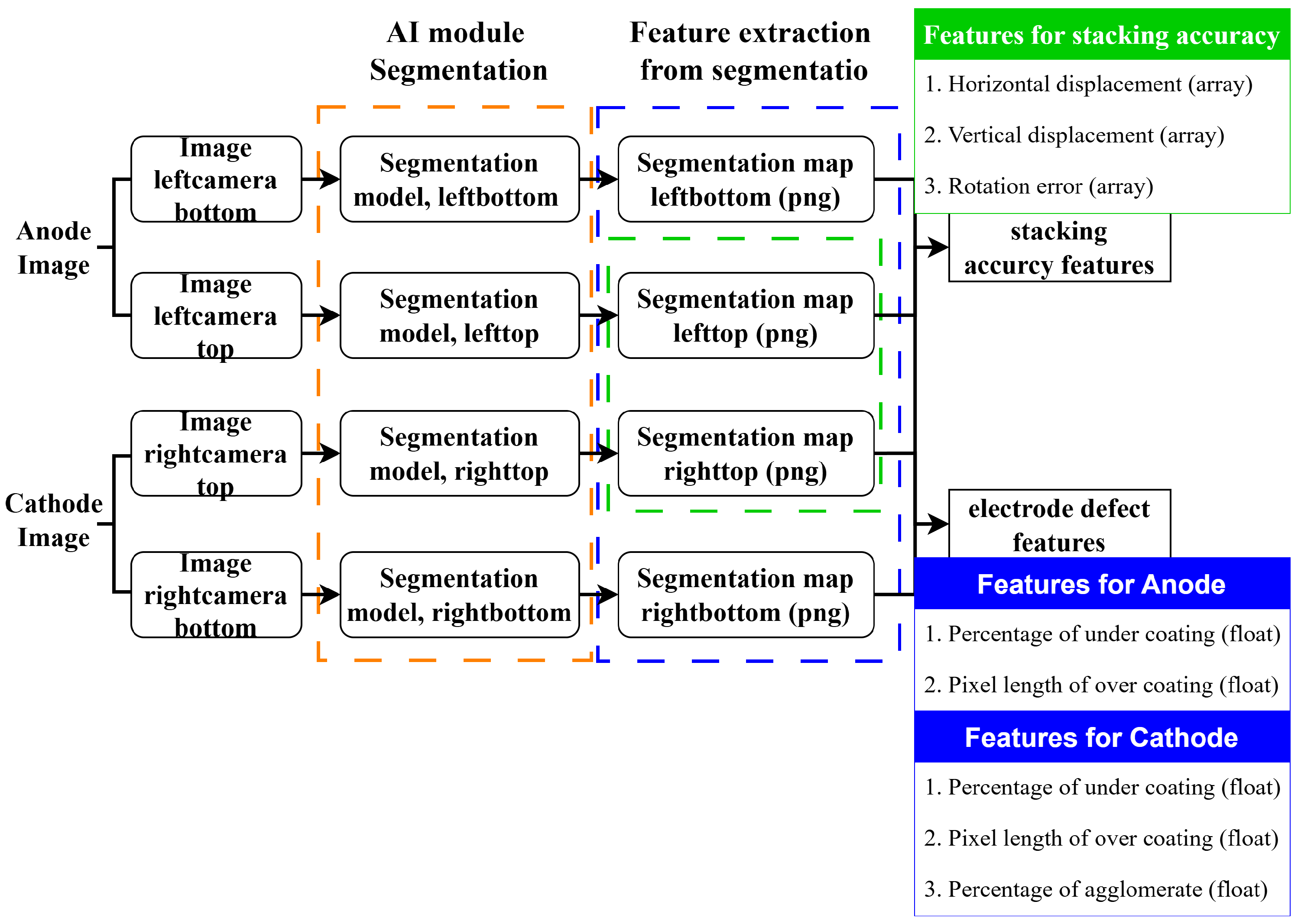Figure 4 demonstrates the feature extraction workflow using the image data collected for electrode defect monitoring as an example.

In this workflow, the raw data collected from LIB assembly are electrode images in JPEG format. Trained segmentation models are adopted to perform semantic segmentation on newly acquired electrode images. Semantic segmentation refers to the process of labeling each pixel in an image to classify the image into multiple segments. It is considered a pixel-level classification technique in image processing, providing higher accuracy than image classification or object detection. For anodes, apart from the irrelevant background, the goal of segmentation is to categorize the coating area and the conductive sheet made of copper. For cathodes, the background, the coating area, the conductive sheet made of aluminum, and the material-agglomerate of the coating material are considered.

Additionally, the positioning of the separators during the stacking process also needs to be determined through image recognition. However, the segmentation map remains too complex and voluminous for the quality analysis supported by the volume of pilot production data. Therefore, simplified numeric features are extracted for use in subsequent data analysis processes. For electrode sheets in the lithium battery assembly process, coating defects, including both overcoating and undercoating, are identified by the correlation matrix as strongly related to battery performance. Additionally, agglomerates appearing on the cathode are also extracted as numeric features. These feature extraction processes effectively reduce the dimensionality by compressing an image into a single numeric value. However, the segmentation map remains overly complex and voluminous in terms of the data volume arising from pilot production. As a result, simplified numeric features are desired in subsequent data analysis.

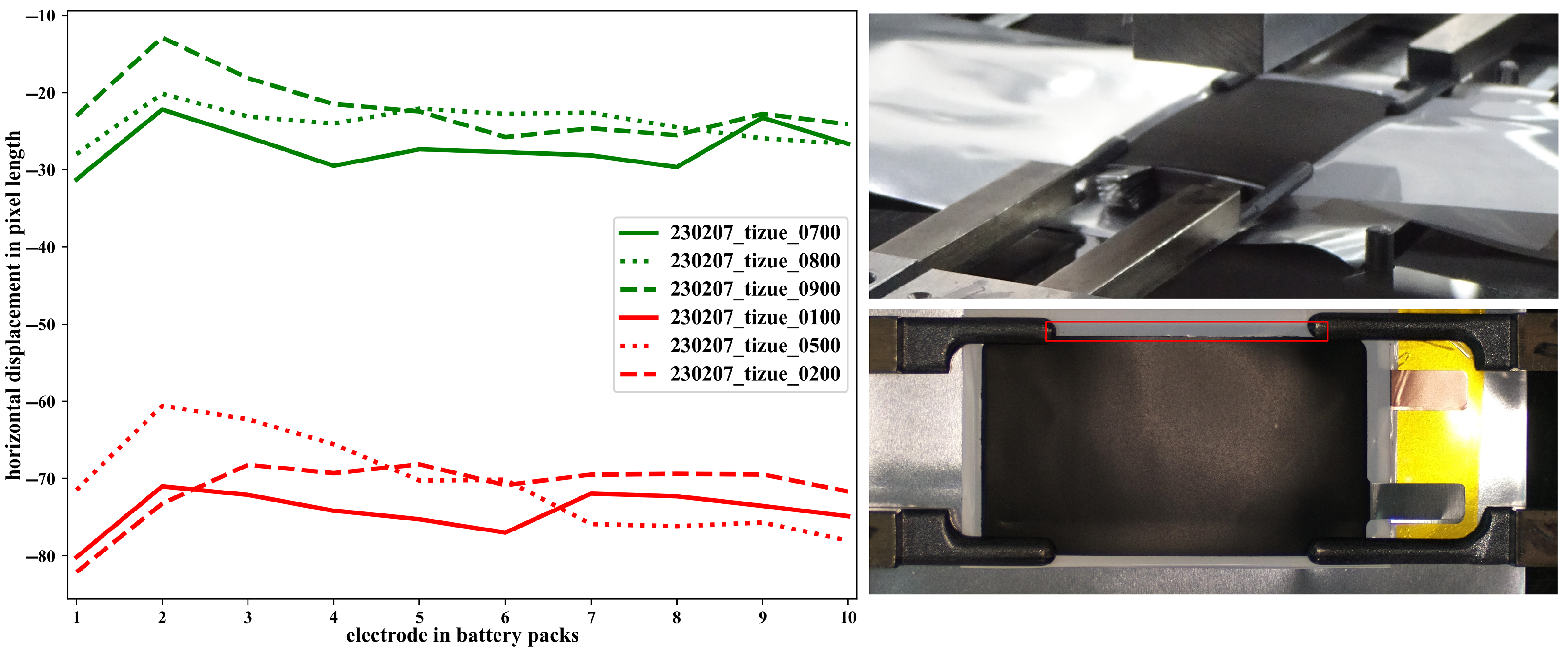
For electrodes in the LIB assembly process, coating defects, including both overcoating and undercoating, and agglomerates appearing on the cathodes are identified by the correlation matrix as strongly related to battery performance. Such feature extraction effectively reduces the dimensionality by compressing each image into a single numeric value. Stacking accuracy in the LIB assembly process is another process factor that correlates with battery performance. The LIB cells assembled on this pilot production line consist of five cathodes and six anodes. Therefore, stacking features should describe the entire cell pack. Features for stacking accuracy are defined by the relative displacement (horizontal and vertical) of each cathode with respect to the anode directly beneath it. For the entire cell pack, the final coating characteristics and stacking accuracy can be regarded as array-type data. Compared to the initial image data, array-type data is more suitable for analysis when dealing with smaller data volumes. Figure 5 demonstrates LIBs with varying stacking accuracy based on the horizontal displacement feature extracted from the images.

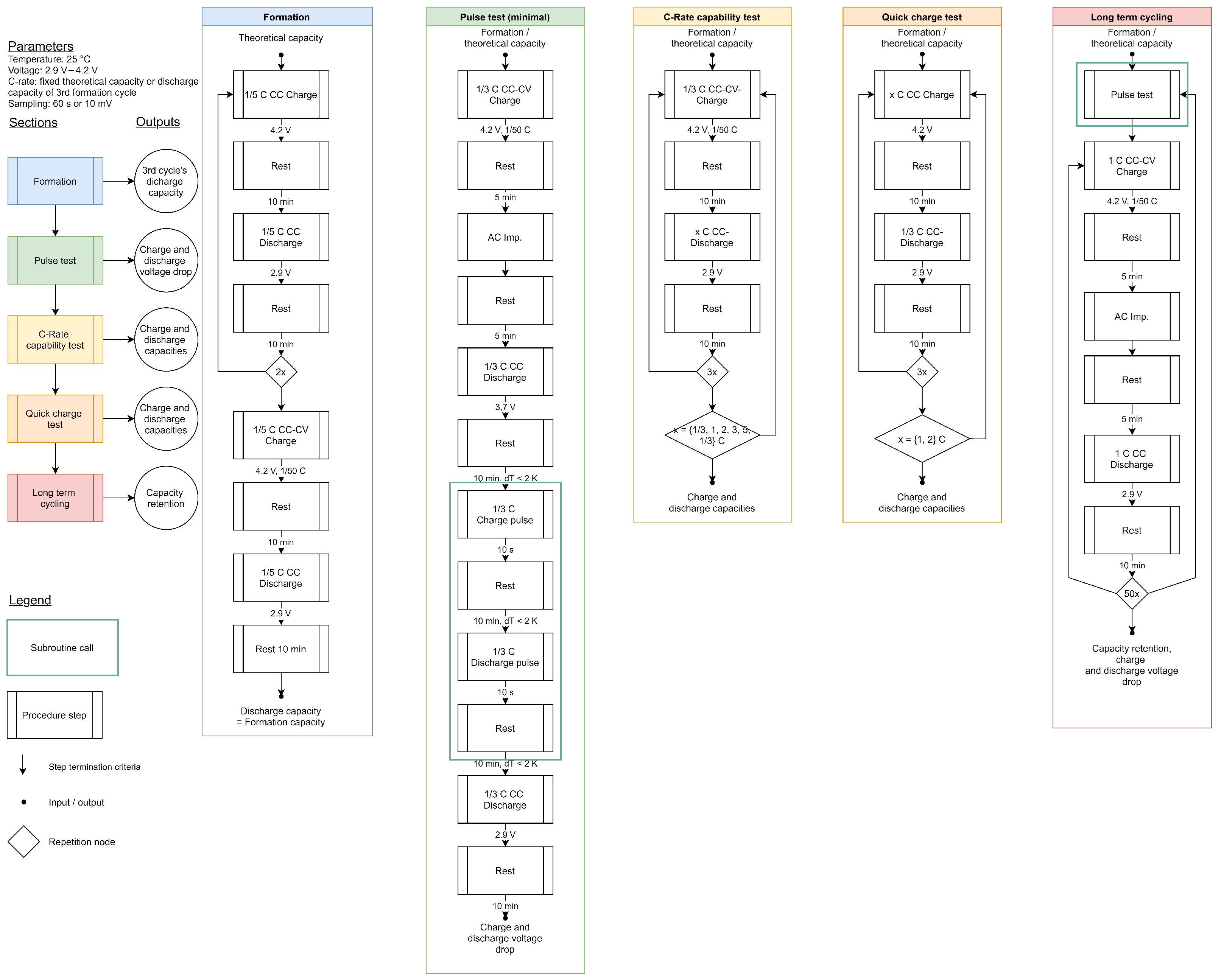
As can be seen in the figure, the horizontal displacement feature clearly distinguishes LIBs with different stacking accuracies. On the quality side, the battery’s performance, obtained from cyclic tests as time-series data, also needs to be compressed to suit small data scenarios. The cycling procedure and the discharge capacity of an example battery cell during the cycling test are provided in Figure 6. Electrochemical features closely related to cell quality were extracted as FQIs for assessing the performance of the produced LIB cells. The process parameters and quality indicators specifically considered in this work are shown in

Table 1. Process parameters, corresponding process features, and final quality indicators.

Process Step	Process Parameter	Process Feature	FQIs
Separation	Coating defect	Under- and overcoating (anode, cathode)	—
Drying	Residual humidity	Drying time	—
Stacking	Stacking accuracy	Horizontal, vertical displacement	—
Filling	Electrolyte amount	Electrolyte amount	—
Cycling test	—	—	Discharging capacity, cell resistance, open-circuit voltage after formation

. Process features refer to input variables derived from process parameters, which are directly applicable for data analysis. For each produced LIB cell, the values of its process features are collected to construct a final dataset for data analysis. Correlation analysis and the development of predictive models for quality control were conducted for some of these quality indicators.

3.4. DOE Plan with Limited Data Volume

Purpose-built datasets for ML modeling with DOE may address two possible directions [26]:

• Finding the optimal values of process variables that give rise to an optimal response
• Exploring the defined parameter space around the optimal values to generate knowledge for monitoring, anomaly detection, and overall quality control

Prior to the realization of stable large-scale production, research and pilot-scale production primarily intend to acquire process expertise, optimize process parameters, or develop a quality control system for the production line. Accordingly, the prepared dataset should not be limited to a parameter space centered around a presumed optimum, but rather be designed to facilitate comprehensive exploration of the entire parameter space. Moreover, the concept of flexible production, which emphasizes increasing the adaptability and variability of the manufacturing process, necessitates a wide exploration of the parameter space during pilot production to identify potentially acceptable sets of process parameters. Therefore, this work focuses on the second direction in dataset construction.

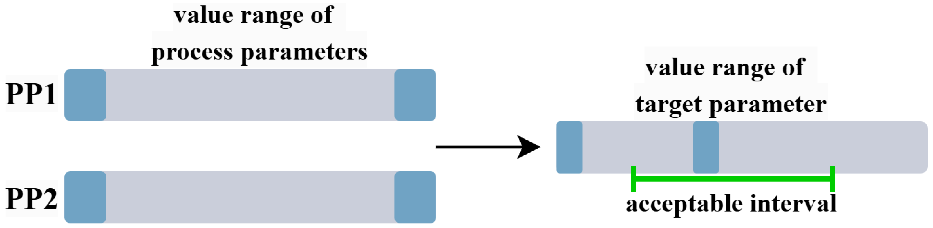
Figure 7 presents a representative example that demonstrates the advantages of exploring a wider range of process parameters in pilot production. The blue regions represent the edge regions within the value ranges of PP1 and PP2, referring to extreme values (maximum or minimum) of the process parameters. When considered individually, an extreme value of a single PP may cause the target variable to fall outside the acceptable range. However, since PPs have a combined effect on the target variable, it is possible that certain combinations involving extreme values—or a single extreme value paired with appropriate settings of other PPs—can still result in acceptable outcomes. These acceptable PP sets do not have to be the optimal solutions within the entire parameter space. Instead, they provide more possibilities and greater flexibility to cope with potential changes.

When the total available data resources are fixed, the chosen DOE strategy for an expanded parameter space should distribute the data points with higher efficiency. Therefore, traditional statistical DOE strategies may no longer be applicable in this context. Space-filling design and iterative sampling have shown advantages, particularly in small-data scenarios [27]. Iterative active learning DOE strategies are more flexible than Space-filling strategies: they can continuously generate additional data points besides existing data. In contrast, LHD requires that the amount of data volume be specified at the beginning, which is not compatible with additional data generation [28]. However, iterative structure is not always the optimal choice. It has to start with an initial amount of data for subsequent iterations. If the model trained with the initial dataset does not drive active learning correctly, then the results of the iterations can be disastrous [29]. Moreover, iterative schemes are difficult to apply when data acquisition is time-consuming. For example, it may take over a month for the entire LIB cycling procedure to obtain a complete quality assessment [30]. In such a case, the time cost of an iterative scheme that considers one new data point at a time is unacceptable. Even if it iterates with batches, this time delay cannot be managed within the project’s timeline.

In this work, the Latin Hypercube Design (LHD) strategy was chosen for data planning. Two independent batches of production were carried out, and the related process as well as quality parameters were collected. LHD strategy was adopted as the data generation scheme for these two batches. According to the selected DOE plan, the first batch was expected to contain 70 cells, and the second batch was expected to contain 30 cells. Finally, the actual number of data points available for analysis was 67 for the first batch and 21 for the second batch. The dataset generated in this work is attached in the repository: https://github.com/xinchengxxc/KIproBatt_dataset (accessed on 20 July 2025).

3.5. Feature Selection

Table 1 presents the process parameters considered according to the DSM, along with the corresponding process features used in data analysis. The key quality indicators considered in data analysis are also listed.

As listed in Table 1, the discharging capacity refers to the cell discharging capacity obtained during the first long-term cycling test (the 25th cycle); the OCV is defined as the OCV abtained after formation procedure (after the 3rd cycle); the cell resistance is derived from the first pulse test (the 4th cycle). These FQIs were identified as the target parameters to be predicted. As for the process features, it should be noted that the features regarding the coating defect should apply to the pouch cell as a whole rather than to each electrode sheet in the cell. Thus, the process feature for coating defect for each pouch cell is characterized by a summary of the features of the electrodes it contains, presented as an average or maximum. Feature correlation analysis and modeling are performed solely on the training dataset with data points from the first batch. Data from the second batch serves as an additional independent test set for the evaluation of the trained predictive models.

Before starting the modeling, data-driven feature selection was conducted to quantitatively analyze the interrelations between quality data and process features. In this study, we used Spearman correlation coefficient [31] and the r-Boruta feature selection method, which is suitable for scenarios with small data sets, to perform feature selection [32].

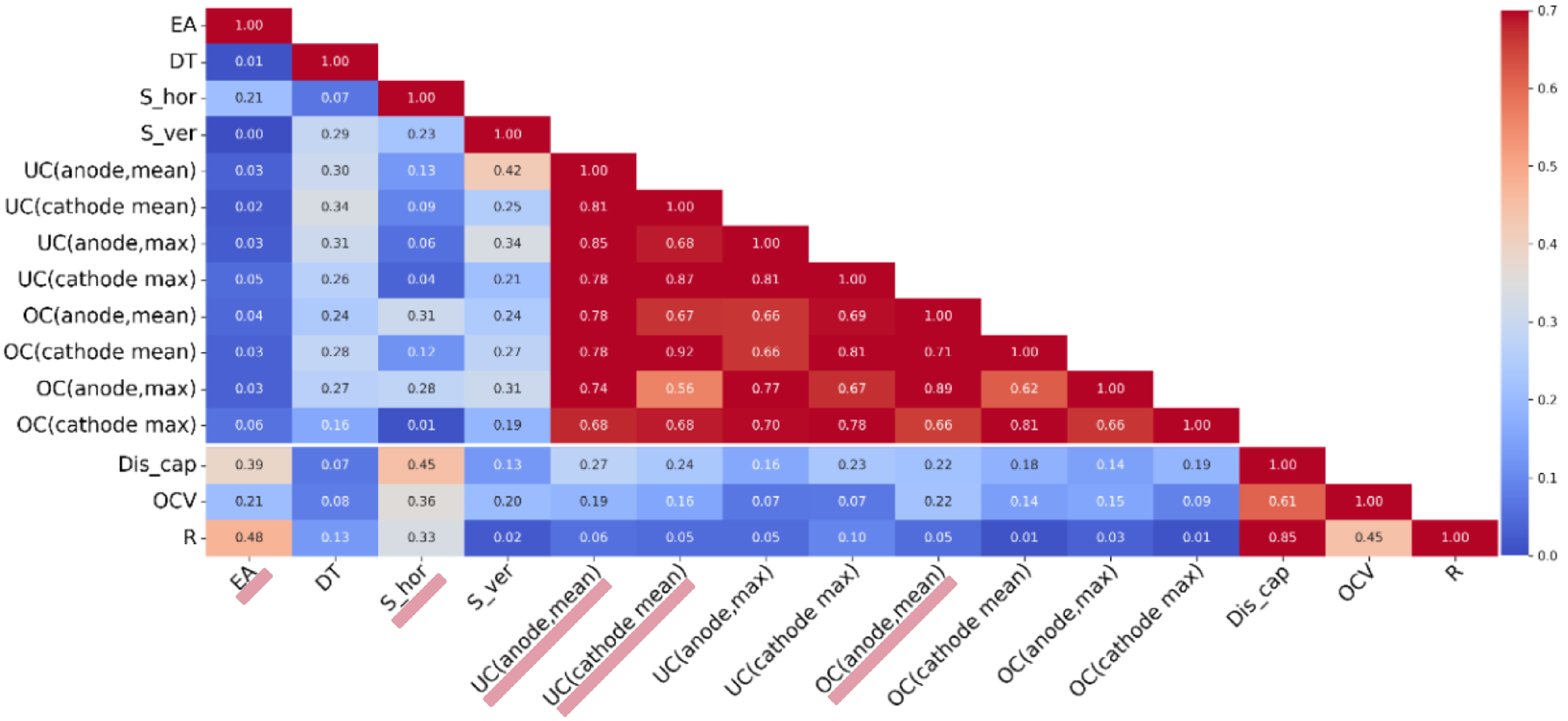
The heatmap based on the Spearman correlation coefficient is separated into three parts. The first block (upper triangular region) records the inter-correlations between process parameters, the second block (lower rectangle area) records the correlations between process parameters and FQIs, and the third block (right triangular region) records the inter-correlations between FQIs. As shown in Figure 8, it is evident that the features related to coating defects extracted from the images exhibit high intercorrelations (dark area in the triangle on the left). Highly correlated features need to be screened for considerations of maintaining independence between input features and to reduce data demands for modeling. Therefore, the mean series features for coating defect, which have a higher correlation with the quality parameters, were retained, while the max series features were excluded.

On this basis, model-based correlation analysis methods are employed to further filter out process features with low correlation to the target parameters. r-Boruta is a wrapper-based feature selection algorithm built upon Random Forest [33]. For each original feature, r-Boruta generates a corresponding ‘shadow feature’ by randomly shuffling the feature values (column-wise), assuming that these shadow features have no correlation with the target parameter. Based on this assumption, r-Boruta constructs a selection criterion to identify and retain only those features that are significantly associated with the target. Only when the importance of a real feature surpasses that of all shadow features is the significance of this feature acknowledged. However, with small sample sizes, using a standard p-percentage in Boruta may risk over-deleting variables due to chance correlations. In a modified approach, r-Boruta calculates p-percentage by setting it based on the maximum correlation with the response variable, reducing the risk of over-deletion when sample sizes are small.

Table 2. r-Boruta feature selection with discharging capacity as target parameter.

r-Boruta Hyperparameter	Selected Process Features
verbose = 2	Electrolyte amount
max_iter = 70	Horizontal displacement (stacking)
perc = 42.5	Under_coating_mean (anode)
—	Over_coating_mean (anode), Over_coating_mean (cathode)

records the parameters inside r-Boruta and the results of the feature selection with discharging capacity as the target FQI.

By examining Table 2 and Figure 8, it can be observed that the feature selection results of r-Boruta align with those of the Spearman correlation coefficient: the Spearman correlation coefficients between the process parameters selected by r-Boruta and the discharging capacity are all above 0.2.

3.6. Establishment of the Predictive Models

Auto-sklearn [34] was employed to build predictive models for the three quality indicators independently. Auto-sklearn with the same parameter settings is adopted to model both the selected features and the original features. All modeling tasks were performed on a workstation equipped with an Intel Core i7-10700 CPU running at 2.90 gigahertz. Considering that the dataset is a small-scale dataset, a modeling time of 400 s was set for each modeling task to prevent overfitting.

Table 3. Auto-sklearn parameter settings for regression modeling.

Auto-Sklearn Parameter Setting	Value/Description
Total time allocated for the task	400 s
Maximum time per model training run	40 s
Initial configurations via metalearning	25 configurations
Memory limit	4096 MB
Resampling strategy	Cross-validation
Resampling strategy arguments	folds: 5
Number of parallel jobs	2

presents the parameter settings used in Auto-sklearn for model establishment.

Table 4. Performance of the predictive models on the test set.

ML Models	RMSE (Test)	R2 Score (Test)
Discharge Capacity
with 5 r-Boruta features	0.019	0.664
with 8 selected features	0.024	0.460
with all features	0.028	0.292
Open-Circuit Voltage
with 3 r-Boruta features	0.012	0.502
with 8 selected features	0.021	<0
with all features	0.065	<0
Cell Resistance
with 6 r-Boruta features	0.013	0.585
with 8 selected features	0.020	0.167
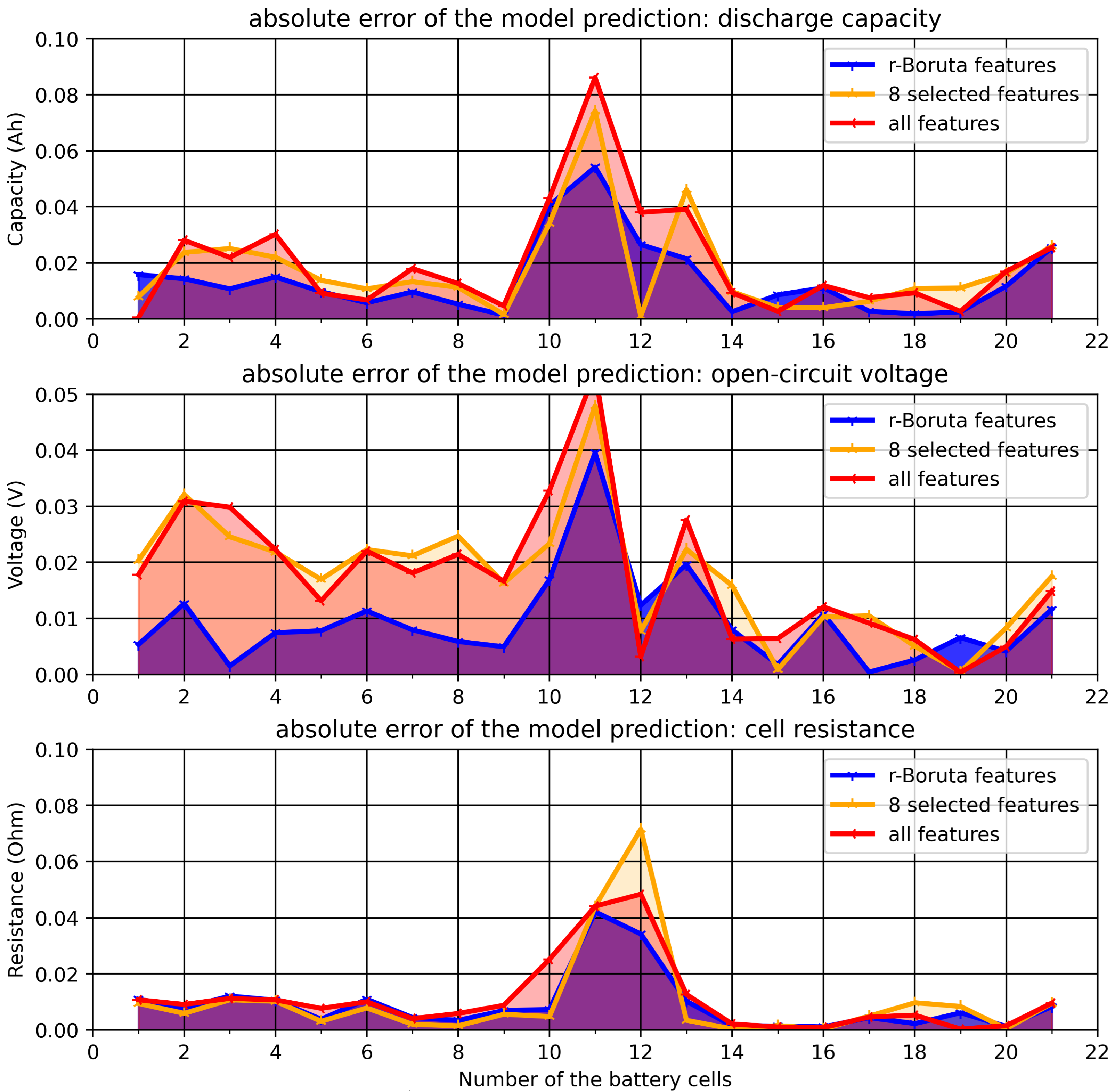
with all features	0.017	0.366

presents the R-squared scores and root mean square error (RMSE) for each model on the test dataset with cell discharge capacity, cell resistance, and OCV as target parameter respectively.

Figure 9 illustrates the absolute error in the prediction of models with different process features for different target parameters. The performance of trained models on the test data indicates that the feature selection process effectively enhances the generalizability of the predictive models.

3.7. Deployment of the VQG for Early Rejection of Low-Performance Cell

The manufacture of LIB is energy intensive and therefore efforts are made to reduce energy consumption in line with the greenhouse gas reduction targets set by the European Union [35]. There is a need for material reduction and inline recycling to increase material efficiency. The early elimination of insufficient cells by avoiding unnecessary production steps contributes to both of these goals. In the conventional VQG framework, quality control is conducted through in-process threshold-based virtual quality gates [36]. Product properties at intermediate process steps are assessed with respect to predefined value ranges of process parameters. If an intermediate process feature falls outside its tolerances, the product is labeled unqualified and rejected. By utilizing machine learning predictive models, it is feasible to forecast LIB final quality indicators during the production process while assessing a broader range of process characteristics. However, by employing ML-based predictive models, it becomes possible to predict the FQIs during production, evaluating a larger collection of process features simultaneously. Such data-driven frameworks replace the threshold-based VQG with model predictions. At a specific stage of the process, an ML model can create VQGs by adopting currently available process features for the predictions of final quality indicators. For newly manufactured LIB cells, the trained model can predict potential future FQIS based on provided process parameter values. However, the final quality outcome is still influenced by the process parameter settings applied in subsequent production steps. The quality control in production is conducted with the following steps. First, quality criteria of the FQIs must be defined. As shown in Figure 10, cells with a discharge capacity below 0.4 Ah or an internal resistance above 0.15 Ω are classified as inferior. For the OCV after formation, the acceptable value range is between 3.2 V and 3.275 V. The quality criteria were assessed by experts based on the obtained data. Then, model-based quality prediction is performed at the end of each process step to forecast the potential FQIs of the product.

Figure 10 presents a visualization of VQG-based quality control for three cells produced on the pilot production line. The cell with ID KI-230718-0400 (subplot (a)) is a qualified product. The predicted FQI values remain within the acceptable quality range at each stage during the production process. In terms of discharge capacity, for instance, the predicted optimal discharge capacity (i.e., the highest achievable value) consistently meets the quality criteria for discharge capacity across all stages from separation to post-filling. Therefore, this cell is classified as qualified. Subplot (b) shows an example of a defective cell (ID KI-230720-0300). Based on discharge capacity, the trained model predicts that its optimal achievable discharge capacity after separation falls below the established quality criteria, meaning it can be classified as defective right after the separation stage. Additionally, based on cell resistance, this cell can also be identified as defective after the filling stage. For a product to be considered qualified, each predefined FQI must meet the specified quality criteria. Subplot (c) on the far right shows another example of a defective cell (ID KI-230911-0300). After the stacking stage, its predicted optimal discharge capacity falls below the specified quality criteria. Therefore, this cell should be classified as defective after the stacking process. If the predicted FQI range falls entirely outside the preset quality criteria, the battery manufacturing process cannot be successfully completed with any production procedures. This triggers an early rejection of the battery immediately after this process. However, if producing lower-performance secondary batteries is justified by different business objectives, the battery can be labeled as a secondary product and continue through the production process.

Taking substandard cells as positives, Figure 11 demonstrates the predictive capability of the three prediction models after filling from the perspective of identifying substandard cells. All FQIs need to be considered in the final determination of whether a battery is qualified. A battery shall be deemed qualified only if all its FQIs fall within their specified thresholds.

Table 5. Precision and recall of the VQG-based quality control.

Production Stage	Separation	Stacking	Filling
Precision	80%	88%	83%
Recall	36%	73%	91%

provides the precision and recall for the VQG-based quality control at each production stage. Attention should be put on precision at each stage, which represents the proportion of predicted substandard batteries that are truly substandard.

The precision values for this VQG-based quality control at each stage of the production have all exceeded 80%. This performance is considered acceptable considering the limited data resource [37]. In general, the recall value reflects the proportion of substandard batteries that are correctly identified as substandard. However, in the VQG-based quality control system, a defective battery does not necessarily indicate that it was defective at earlier stages of production. Some unqualified batteries may have become defective due to inappropriate process parameters in subsequent stages (e.g., during the filling process), which caused them to fall out of qualified thresholds. The recall values in Table 4 increase as the production progresses, reaching 91% after the filling stage. This suggests that the VQG system is capable of identifying the vast majority of defective batteries by the end of the production process.

4. Conclusions

This article presents the development and implementation of a CPS for quality control in the pilot production of lithium-ion batteries. The proposed system consists of process sensors, an ontology-based data space, and a data infrastructure, all integrated into a pilot assembly line that supports the creation of a machine learning-based predictive model for the early detection and evaluation of battery quality. The impact of limited data volume on data-driven solutions was mitigated by preparing the dataset using appropriate DOE strategies. The proposed ontology-based data space enables a transparent overview of the entire data flow and offers an effective way to address challenges caused by potential errors in the data during the pilot production stage. The VQG-based quality control system ensures real-time, data-driven quality control by systematically identifying and analyzing quality-related process parameters. The article focuses on the common issue of data volume limitations in pilot production environments. Selecting appropriate DOE strategies for experiment/production planning, as well as performing dimensionality reduction and feature selection during data analysis, can enhance the efficiency of data analysis, enabling modeling tasks to be accomplished with small data. Results indicate that the proposed VQG framework successfully predicts end-of-line quality, which can improve flexibility and energy consumption efficiency for the adaptation of variations. As a subsequent step, the VQG quality control system developed in this study will be tested and improved in a more industrially relevant production environment with an expanded scale.