Abstract
Developing efficient recycling processes with high recycling quotas for the recovery of graphite and other critical raw materials contained in LIBs is essential and prudent. This action holds the potential to substantially diminish the supply risk of raw materials for LIBs and enhance the sustainability of their production. An essential processing step in LIB recycling involves the thermal treatment of black mass to degrade the binder. This step is crucial as it enhances the recycling efficiency in subsequent processes, such as flotation and leaching-based processing. Therefore, this paper introduces a Representative Black Mass Model (RBMM) and develops a computational framework for the simulation of the thermal degradation of polymer-based binders in black mass (BM). The models utilize the discrete element method (DEM) with a coarse-graining (CG) scheme and the isoconversional method to predict binder degradation and the required heat. Thermogravimetric analysis (TGA) of the binder polyvinylidene fluoride (PVDF) is utilized to determine the model parameters. The model simulates a specific thermal treatment case on a laboratory scale and investigates the relationship between the scale factor and heating rate. The findings reveal that, for a particular BM system, a scaling factor of 100 regarding the particle diameter is applicable within a heating rate range of 2 to 22 K/min.
1. Introduction
The demand for lithium-ion batteries (LIBs) has risen significantly in recent years and is anticipated to persist for decades to come, as indicated by a study conducted by the Fraunhofer Institute for Systems and Innovation Research (ISI) [1] in 2022. However, with the global demand for LIBs on the rise, the demand for their essential components is also increasing. This scenario could result in a shortage of the necessary supplies required for the production of LIBs.
The EU has compiled a list of critical raw materials [2]. In particular, one critical raw material on this EU list is graphite, which is a major component in LIBs, with approximately 20 wt.% [2,3].
Therefore, it is of crucial interest that spent LIBs are recycled with high efficiency [4,5]. This action can significantly reduce the raw material supply risk for LIBs and increase the sustainability of their production. It is therefore important and prudent to develop efficient recycling processes with high recycling quotas to recover also graphite and other critical raw materials contained in LIBs. One possible schematized recycling route for spent LIBs is shown in Figure 1.
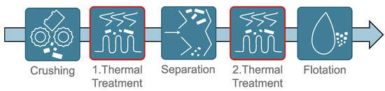
Figure 1.
A possible schematized recycling route for spent LIBs based on [6,7,8].
After discharging and then dismantling the spent LIBs from their protecting casing, the LIBs are crushed and treated with heat, typically under a vacuum, to release the volatile components, such as the electrolyte solvents [8]. The tailored release of the electrolyte solvents seems particularly important, which makes the understanding of vapor–liquid equilibrium (VLE) under representative process conditions necessary [9]. After these first crushing- and drying-based processing steps, the crushed and dried mass can be separated into coarse and fine fractions by mechanical processing [8]. The coarse fractions typically consist of iron, plastic, aluminum and copper [8]. The fine fraction is typically called black mass (BM) and consists mainly of the active material, such as graphite or lithium metal oxide (LMO) [8]. The BM also contains the binder material and may contain the remaining low-volatility electrolyte solvents [8]. To release the remaining low-volatility solvents and degrade the polymer-based binder, a second heat treatment of the BM can be applied [8]. The tailored degradation of the binder material enhances the purity and recycling efficiency of the graphite and LMOs in downstream processing [10], such as forthcoming flotation-based [7], leaching-based [11,12], and other possible recycling steps [13]. Vanderbruggen et al. [7] showed that, with a thermal treatment decomposing the binder and releasing the agglomerates of the active material, flotation achieved graphite recovery of approximately and LMO recovery of nearly . Compared to this, pure mechanical pre-treatment could achieve graphite and LMO recovery of approximately [7].
Therefore, binder degradation seems to be an important processing step to increase the recycling efficiency of LIBs. Among other possible binder materials in the BM, such as carboxymethyl cellulose (CMC) and styrene butadiene rubber (SBR), the binder polyvinylidene fluoride (PVDF) is a common binder material for the active material in LIBs due to its exceptional thermal stability. Therefore, a typical BM composition obtained from recycling processes is likely to contain PVDF, which is one reason that we have considered PVDF in this work. The challenge is that, on the one hand, the binder should be degraded by thermal treatment in a certain amount of processing time and, on the other hand, other valuable components should not be decomposed [8]. Furthermore, the thermal treatment of the BM can release toxic gases such as hydrogen fluoride (HF), which can cause the corrosion of equipment and air pollution by decomposing the fluoride-containing components in spent LIBs, such as the binder PVDF, which must be considered in experimental security management [6]. Moreover, two common thermal processes are used to degrade the binder, calcination and pyrolysis, and an overview of industrial recycling routes can be found in [14]. Pyrolysis is more effective than calcination in preventing undesired graphite decomposition due to the absence of oxygen in the atmosphere [6,15,16,17,18], which is one particular reason for our focus on pyrolysis conditions in this work. In order to tailor the binder degradation during the thermal treatment of black mass, efficient computational methods are necessary to optimize future thermal treatment processes and adapt flexibly to changing feeds in the recycling route.
Therefore, the goal of this work is to develop the first computational model framework capable of simulating the degradation of polymer-based binders in black mass under an inert atmosphere, which is encountered in thermal processes, where heat transfer phenomena and the time and space fields of the temperature and black mass motion is considered. To achieve this goal, herein, an isoconversional kinetics approach [19] is directly coupled with the discrete element method (DEM). One challenge thereby is that BM particles typically have a mean particle size of approximately 10 µm, as shown in the work by Vanderbruggen et al. [20]. Therefore, a coarse-graining approach is additionally applied in connection with a representative black mass composition to allow scaling, termed the Representative Black Mass Model (RBMM). Therefore, with lower computational costs, the physical thermal treatment times can be calculated.
Principal isoconversional approaches are described in Vyazovkin et al.’s guidance [19]. This guidance explains how to determine kinetic parameters from thermogravimetric analysis (TGA) and perform isoconversional calculations [19]. To perform these calculations, methods such as model-free and model fitting are used [19]. There are several model-free methods for the determination of activation energy from reactions without assuming any form of reaction model, including the Friedman [21], Ozawa–Flynn–Wall (OFW) [22,23], Kissinger–Akahira–Sunose (KAS) [24], and Vyazovkin methods [25,26,27]. The isoconversional approach allows the determination of the overall kinetics of a physical property change, such as the degradation of a polymer-based binder, without requiring knowledge of the species-specific reactions of molecules [19]. In this work, the OFW method is used and coupled with DEM.
DEM is a numerical technique used to calculate the movement, acting forces, and heat transfer phenomena of discrete elements within CAD geometries [28]. Its main application is to investigate and predict the behavior of bulk materials in a specific geometry [28]. To simulate bulk materials with small particle diameters, such as powders, a coarse-graining (CG) scheme can be used to reduce the number of particles and increase the computational efficiency [29]. An example of a CG scheme is the one proposed by Bierwisch et al. [29], which is also the scaling concept used in this work to develop the RBMM.
With the developed computational framework, the first survey of thermal treatment cases in a lab-scale environment is established, where the focus is on understanding the scale parameters and heat transfer on the lab scale and performing model validation.
2. Materials and Methods
2.1. Materials
The binder material under investigation was a powder of polyvinylidene fluoride (PVDF-CAS No.: 24937-79-9), purchased from Sigma-Aldrich (Saint Louis, USA). The characterized properties, i.e., average molar mass , density , melting temperature , glass transition temperature , and degradation temperature , are listed in Table 1.

Table 1.
Physical properties of the investigated PVDF powder according to Ref. [30].
2.2. Experimental Procedure
Thermogravimetric analysis (TGA) was performed using a modified high-pressure simultaneous thermal analysis device (HP STA) from Linseis GmbH. The initial sample mass of the investigated PVDF was approximately 10 mg. The sample atmosphere was N2 at a gas flow rate of 0.9 L/min. The degradation of the PVDF powder was investigated at three heating rates (HR) of 2.0 K/min, 10.7 K/min, and 22.8 K/min in the temperature range of 20
°C to 600 °C.
2.3. Computational Methods
In order to describe the degradation of a binder on a larger scale while also considering motion during the thermal treatment process, a Representative Black Mass Model (RBMM) is developed and treated in a thermal process to degrade the binder by coupling the binder thermal degradation kinetics with DEM and by applying a coarse-graining scheme.
2.3.1. Thermal Degradation Kinetics
The Ozawa–Flynn–Wall (OFW) method, developed independently by Ozawa [22], Flynn, and Wall [23], is used to calculate the activation energy as a function of its extent of conversion from TGA data at constant heating rates. Therefore, the TGA data are converted to the extent of conversion [19]:
where is the initial mass, is the final mass, and is the current mass at time t. The extent of conversion is a scalar variable and describes the state of the degraded sample in a range from 0, i.e., no degradation occurring, to 1, i.e., degradation completed [19].
To calculate the kinetics, the following differential equation is given to evaluate the extent of conversion over time [19]:
where is the conversion rate, is the heating rate (HR), is the reaction rate, and is the reaction model.
The reaction rate is described by the Arrhenius equation [19]:
where A is the pre-exponential factor and R is the universal gas constant.
From Equation (2) and the constant HR , the OFW method yields the following equation [19]:
where is the integral form of the reaction model [19]:
In a linear plot of over , the activation energy can be determined by calculating the slope for the same extent of conversion [19]. The pre-exponential factor A can be calculated from the intercept [19]. To calculate the intercept, a proper reaction model must be applied and the parameters must be determined [19]. Vyazovkin et al. [19] recommend that at least 3–5 TGA measurements at different heating rates are required to determine the activation energy . A suitable reaction model, which is applied in this work, is the reaction order model according to Ref. [19]:
where n is the reaction order and the parameter to be determined.
2.3.2. Discrete Element Method (DEM)
DEM is a numerical method based on Newton’s equations of motion [28]. In general, the DEM approach treats particles as rigid bodies that have six degrees of freedom, the three translational degrees and the three rotational degrees around their center of mass [28]. A comprehensive overview of the DEM approach and its applications is presented in the work of Yeom et al. [28]. In addition to describing particle motion, models are also available to calculate the heat transfer mechanism using the DEM approach [28]. One powerful DEM solver that provides these models is the open-source DEM solver LIGGGHTS-PFM [31], which is also used in this work.
Stability of DEM Simulations
To achieve a stable and accurate DEM simulation, it is recommended to select a time step that is of the maximum time step [28]. The maximum time step can be estimated using the following equation, which is based on the Rayleigh wave [28]:
where is the particle density, R is the particle radius, G is the shear modulus, and is the Poisson’s ratio of the material properties of the DEM particle.
Thermophysical Descriptions
LIGGGHTS-PFM has a linear heat transfer model implemented, which is based on Chaudhuri et al. [32]. This model describes linear heat transfer through conduction, where heat flux occurs between particle i and geometry j or particle j as [32]:
where is the temperature of the particle i, is the temperature of a geometry j or particle j, and is the heat transfer coefficient. Furthermore, this model assumes a homogeneous temperature distribution within a particle [32]. The heat transfer coefficient is given by the following equation [33]:
where and are the thermal conductivities of particle i and particle j or geometry j, respectively, and is the contact area between these two objects. Depending on the model selected, the contact area can be chosen from three modes [33].
- Mode: Calculation according to the overlapping area of objects.
- Mode: Constant by user-defined overlap area.
- Mode: Calculation by projection area , where and is the radius of the smaller object.
Additionally, LIGGGHTS-PFM has a radiation model between particles to simulate radiative heat transfer according to Stefan–Boltzmann’s law [33]. Currently, LIGGGHTS-PFM does not support radiative heat transfer between a geometry and a particle [33]. Therefore, herein, this heat transfer mechanism is newly implemented and it is based on the already implemented radiation model between particles by
where is the radiative heat flux between geometry j and particle i, is the projected area of particle i, is the emissivity of particle i, is the Stefan–Boltzmann constant, and and are the temperature of geometry j and the temperature of particle i.
The evolution of the temperature of the particle i is given by the following equation [33]:
where is the current mass, is the specific heat capacity, and is the heat flux into the particle, with k heat fluxes involving particle i.
Coarse-Graining (CG) Scheme
One sophisticated coarse-graining (CG) scheme is the approach of Bierwisch et al. [29]. This CG scheme scales the original particle radius R to a scaled up particle radius [29]. The ratio of the scaled radius to the original radius R is defined as the scaling factor [29]. Using this method, the number of particles can be reduced to ∼ and the time step can be increased by ∼ [29].
The main idea of this approach is to use the same energy density for the scaled particles and the original system, and this can be achieved by the following conditions [29]:
where is the density of the original particle and is the density of the scaled particle.
Moreover, the condition of the volume fraction is [29]
where is the volume fraction of the original system and is the volume fraction of the scaled system.
2.3.3. Representative Black Mass Model (RBMM)
BM is mixed waste, and various compositions can occur depending on the LIB input mixtures. Therefore, in this work, a Representative BM Model (RBMM) is introduced to take into account, on the one hand, the variety of compositions in BM and, on the other hand, the scaling of the particles, such that they become treatable in terms of computational costs for future thermal processing simulations. Regarding the composition, it is carried out for one particular example. This section describes the model assumptions of the RBMM, combining the isoconversional kinetics and DEM with the coarse-graining scheme.
Figure 2 illustrates the concept of the RBMM. Figure 2a shows a sample of BM as bulk material. The BM consists of numerous fine particles of active material from spent LIBs, including the polymer-based binder. These fine particles are agglomerated based on the coarse-graining approach to a scaled particle, which is denoted as RBMM in Figure 2a. For these coarse-grained spherical particles, homogeneous but time-dependent characteristics, i.e., the temperature and extent of conversion , are mapped following Equations (2) and (11). Therefore, the degradation of the polymer-based binder within the BM, due to thermal treatment, can be described in a scaled up particle such that the computational cost for DEM decreases. The coarse-graining approach applied to the BM is displayed in Figure 2b.
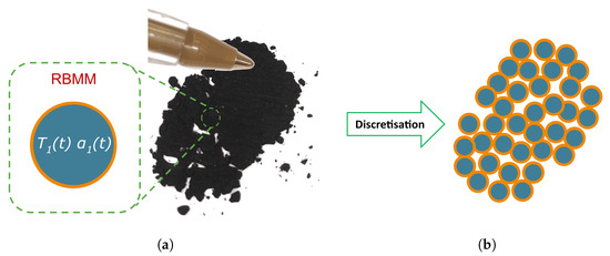
Figure 2.
Coarse-graining of BM to generate RBMM. (a) Real BM with the coarse-graining approach. (b) Discretized RBMM particles for higher-scale simulations.
These RBMM particles result in a field of properties in space and time that interact with each other in the DEM environment. Interactions involve the movement of the RBMM particles as well as the respective heat transfer.
As introduced above, herein, the approach of Bierwisch et al. [29] is applied:
where is the initial density of the RBMM particle and is the density of the BM.
Therefore, the initial mass of the RBMM is calculated by
where is the diameter of the scaled RBMM particle and the term in the parentheses is the volume of the RBMM particle.
To account for the mass reduction in the RBMM due to the degradation kinetics of the BM, there are two possible approaches. The first approach is to adjust the diameter and the second is to adjust the density to the current mass . In this work, the second approach is chosen, according to numerical advantages such as the stability of a DEM simulation with respect to the maximum time step (Equation (7)).
This results in the following equations:
where is the residual weight fraction of the treated BM:
where is the final mass and represents the initial mass from a TGA measurement of the BM to be modelled.
To describe the thermal transfer of the RBMM particles, three heat transfer mechanisms are considered and illustrated in Figure 3.
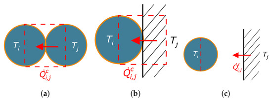
Figure 3.
Considered heat transfer mechanisms for the RBMM particle. (a) EHT: PP; (b) EHT: PW; (c) Radiation: PW.
The first and second heat transfer mechanisms are considered as effective heat transfer (EHT) between a particle i and another particle j (as shown in Figure 3a, particle–particle (PP)) or a wall element j (as shown in Figure 3b, particle–wall (PW)). The EHTs are calculated using Equations (8) and (9), where, in Equation (9), the thermal conductivity is considered as an effective heat transfer coefficient . To calculate the contact area , the projection area is chosen as the mode. This mode considers the size of RBMM particles and the distance between the objects in contact, represented by i and j, as illustrated by the red rectangular dotted lines in Figure 3a,b. This mode ensures that the effective heat transfer is independent of the particle diameter. The third mechanism of heat transfer is radiation, as illustrated in Figure 3c. Emission is treated as normal from a wall element j. The heat flux is calculated using Equation (10). The implemented heat transfer model for radiation also utilizes the projection area of the RBMM particle to determine the area that participates in heat transfer. By using the projection area, the hull surface of the bulk material is considered, which participates in the radiation heat transfer. Table 2 summarizes the RBMM parameters.
Table 2.
The uniform and homogeneous model properties of the RBMM.
2.3.4. Specific RBMM (sRBMM) for LIBs with a Particular Composition
To simplify and reduce the number of measurements required for the RBMM, a Specific RBMM (sRBMM) is introduced. Therefore, the BM is divided into components that behave inertly in the thermal treatment and only the polymer-based binder is treated as active and can degrade. This leads to
where is the current mass of the binder, and is the initial mass of the inert component i. The can be expressed using the mass Equation (18) from the RBMM, but, instead of the initial and final masses of the RBMM, the initial and final masses of the binder are used.
The initial mass of the inert component i is expressed by
where is the initial weight fraction of the inert component i of the BM.
For the sRBMM, the equation for the specific heat capacity must be adapted to the sRBMM assumption and leads to the following equation:
To take into account the enthalpy of fusion , a common method is to use the approximated Delta Dirac function as used by Bouzennada et al. [34]:
where is the specific heat capacity of a component i with the latent amount of heat . The approximated Delta Dirac function is expressed by [34]
where is the melting temperature of the component i and is the Dirac Delta, which describes the width of the approximated Dirac function.
3. Results and Discussion
This section investigates the PVDF binder degradation on a single particle state of the described sRBMM and further provides the first model calculations and tests for the fully coupled isoconversional kinetics and DEM with the coarse-graining approach, including also the newly implemented complex heat transfer model.
3.1. Determining Model Parameters for the sRBMM
The particular composition of BM is a result of the spent LIB type and the applied recycling process. Assuming that all volatile components are released and the active material is separated from the non-active material, the resulting BM consists of the cathode active material, the anode active material, and the binder.
Mossali et al. [3] determined the possible compositions of spent LIBs. By considering only the components previously assumed, the following composition presented in Table 3 arises. The cathode active material is lithium metal oxide (LMO) and the anode active material is predominantly graphite. According to Mossali et al. [3], the most commonly used binder is PVDF, which is also applied herein.
Table 3.
Particular compositions for sRBMM mapping.
The initial composition of the sRBMM is 8 wt.% for the PVDF, 51 wt.% for the NMC, and 41 wt.% for the graphite. These initial compositions are used to further determine the parameters for the sRBMM, as described in the following section.
3.1.1. Determination and Validation of the Kinetic Model Parameters for PVDF Degradation
The degradation kinetic model parameters for the sRBMM were determined from TGA measurements on samples of PVDF at three different heating rates. Using Equations (1) and (4), the conversion rate and the activation energy were calculated from these measurements. The results are presented in Figure 4, where the TGA measurements are visualized in the --plot. For each point of the TGA measurement, the temperature, the heating rate (corresponding to ), and the extent of conversion are displayed, with the latter being assigned a specific color. The color “red” indicates , i.e., the conversion has already started, and the color “blue” corresponds to , i.e., the conversion is almost finished. By determining the slope for the same extent of conversion for each heating rate, the activation energy can be calculated. These slopes are shown in Figure 4 via lines in the appropriate color. The calculated activation energies are listed in Table 4. Furthermore, the pre-exponential factor A is calculated with a reaction order parameter of , where the parameter shows the best accuracy for degradation predictions for this particular case.
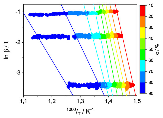
Figure 4.
--plot to determine the activation energy from the TGA measurements of the PVDF binder degradation.
Table 4.
Determined degradation kinetic model parameters for the binder PVDF.
The kinetic parameters for the binder degradation model are now available. With this set of parameters, the TGA measurements can be reproduced by using Equation (2). The calculations are shown in Figure 5 and compared with the experimental data. Figure 5 shows the normalized mass of the curves over the temperature. Equal heating rates are shown in one color, where blue corresponds to a heating rate of 2.0 K/min, green to 10.7 K/min, and red to 22.8 K/min. The symbols (colored squares) represent the TGA measurements of PVDF, and the lines represent the calculations with the isoconversional degradation model. The results show the suitable description of the PVDF’s degradation with the kinetic model, showing a coefficient of determination .
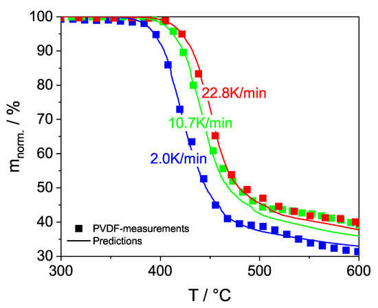
Figure 5.
TGA measurements (symbols) and degradation kinetics model (lines) of PVDF at different heating rates. Model accuracy: .
The combination of the OFW method and the third-order reaction model results in a highly accurate kinetic description, where the heating rate can be considered accurately. An activation energy of = 330 kJ/mol is determined using the OFW method. Comparing this result with the literature data, it is found that a similar activation energy is achieved by Xu et al. [35], with a value of = 260 kJ/mol.
3.1.2. Determining the Parameters for the Mass and the Heat Transfer
The remaining model parameters of the sRBMM are the model parameters related to Table 2. The remaining parameters are determined based on the literature data. They are presented in Table 5. The scale parameter is the diameter of the RBMM. This parameter can be principally adjusted to the particular case. Herein, the scale parameter influence is evaluated on the single particle stage. This choice of diameter allows the scaling of the resolution of the simulation in relation to the simulation time required.
Table 5.
Selected mass and heat transfer parameters of the sRBMM.
The chosen density of the sRBMM particle is estimated by considering the literature data with the density of its main components and the possible porosity of BM. This results in a density for the sRBMM of = 3200 kg/m3.
The effective heat transfer is assumed to be constant over temperature in the currently chosen temperature window. In the paper by Gotcu [46], the results when measuring the effective heat transfer within the bulk material of the active material showed no significant changes in the temperature range from 25 °C to approximately 300 °C, which underpins this assumption.
The emissivity of the bulk material is estimated from the studies of Mohanty et al. [39] and Ho et al. [40]. The first study shows that the emissivity of the bulk material, NMC, has emissivity of approximately , by referring to the emissivity of aluminum foil of approximately [47], and the study by Ho et al. [40] shows the measured emissivity of the bulk material, graphite, to be . Therefore, the emissivity of the sRBMM is assumed to be in this range and is set to .
For each assumed component in the sRBMM, the specific heat capacity is a function of temperature T. Furthermore, the used specific heat capacity equation of the PVDF component does not include the enthalpy of fusion . Therefore, the enthalpy of fusion is additionally taken into account by applying Equation (22).
Figure 6 shows the specific heat capacity for the components PVDF (red), graphite (green), and NMC (blue) and the resulting specific heat capacity for the sRBMM (black) as a function of temperature T. The specific heat capacity is calculated using Equation (21) and its course lies between its main components, graphite and NMC. At 165 °C, the melting peak of PVDF is modelled with an area of 3.2 kJ/kg, which corresponds to of the enthalpy of fusion . This value corresponds to the chosen initial weight fraction of the binder in the sRBMM. This graph shows that the specific heat capacity of all components increases by a factor of approximately 2 in the temperature range from 0 °C to 600 °C. This increase in specific heat capacity demonstrates the importance of considering this effect when designing and optimizing a thermal treatment process.
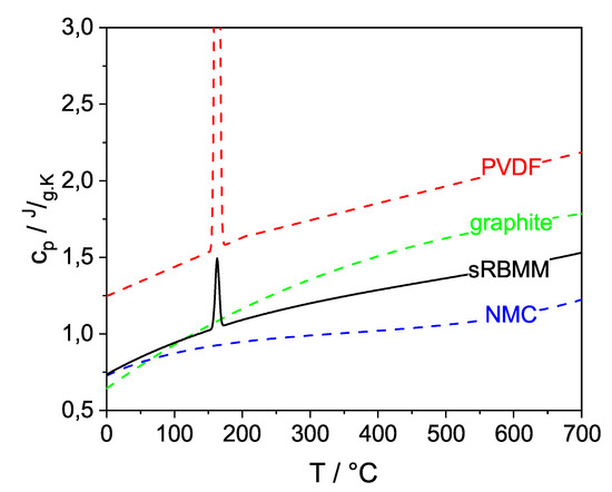
Figure 6.
Calculated specific heat capacities versus the temperature of the main components in the sRBMM and the resulting specific heat capacity .
3.2. DEM Simulations: Investigation and Validation of the sRBMM
The DEM simulations are performed for the sRBMM.
The sRBMM calculations are performed in a heated crucible with a scaled sRBMM particle, where the wall temperature of the crucible is set at a defined heating rate. Figure 7 shows the simulation case with the CAD geometry of the crucible and the sRBMM particle. The calculations are performed for two diameters of the sRBMM particle and for three heating rates of 2.0 K/min, 10.7 K/min, and 22.8 K/min; a total of six calculations are performed and the results are presented. The two diameters considered are = 1 mm and = 10 mm. In both calculations for the different diameters, the ratio of the crucible to the particle diameter is the same at . An overview of the parameters chosen for these calculations is given in Table 6.
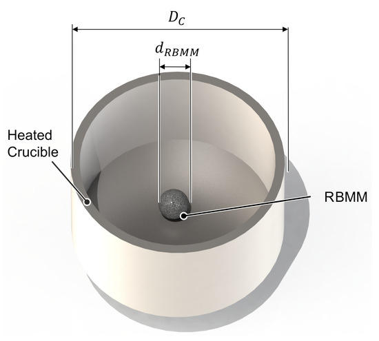
Figure 7.
Simulation case for one sRBMM to investigate the coupled isoconversional kinetics with DEM by applying coarse-graining.
Table 6.
Selected boundary conditions (BC), initial conditions (IR), and parameters for the calculations.
Figure 8 displays the simulation results for the scaling case with a diameter of = 1 mm and a heating rate of 10.7 K/min. Figure 8 is divided into four sections, with each section showing the results at a certain time. In each sub-figure, the wall temperature of the heated crucible is shown in the cross-section, while the current state of the variable extent of conversion is represented by the color of the particle. The color scheme is shown at the bottom of the figure, with blue indicating a wall temperature of 20°C and red indicating 600 °C. The color of the particle changes from black at to white at .
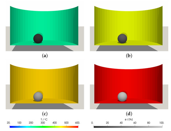
Figure 8.
Calculation results for binder degradation in sRBMM for the diameter = 1 mm and for the heating rate of 10.7 K/min. (a) Temperature = 200 °C, extent of conversion ; (b) temperature = 440 °C, extent of conversion ; (c) temperature = 480 °C, extent of conversion ; (d) temperature wall = 600 °C, extent of conversion .
For instance, Figure 8b illustrates that the wall temperature has reached 440 °C, and the degradation process has started. This can be observed from the extent of conversion , where the value has increased by . Referring to Figure 8c, the wall temperature increased by approximately 40 °C while the extent of conversion increased by . This large increase in the variable is due to the degradation kinetics of the binder PVDF, where the peak temperature for this heating is around 440 °C and therefore the degradation process occurs very rapidly. This effect is also present in the TGA measurements shown in Figure 5. Figure 8d shows that the wall temperature increases by 120 °C, reaching a final value of 600 °C, while the extent of conversion increases by . This behavior maps to the degradation kinetics of the binder PVDF. The kinetics slows down after reaching the maximum. The simulated physical time in this simulation case was approximately 55 min.
Figure 9 shows the TGA results for six calculations, where the diameters and heating rates are varied. Each calculation with the same heating rate is represented by a color (2.0 K/min as blue, 10.7 K/min as green, 22.8 K/min as red), and each calculation with the same diameter is represented by a particular line type. The dotted line represents the calculation with a diameter of = 1 mm, while the straight line represents the calculation with a diameter of = 10 mm. Figure 9a displays the normalized mass over wall temperature . It can be observed that the normalized mass in all cases decreases by approximately . The maximum normalized mass that can be converted for these defined parameters is . Furthermore, it can be observed that increasing the heating rate or the diameter results in a decrease in the amount of converted mass. In the calculation with a smaller RBMM diameter of mm and a lower heating rate K/min, the converted mass reached its maximum of . In comparison, the calculation with a larger RBMM diameter of mm and a heating rate of K/min resulted in a converted mass of , a difference of from the normalized mass . Additionally, the figure illustrates the temperature differences between different diameters at the same heating rate . The temperature gap for K/min is approximately 8 °C; for = 10.7 K/min, it is approximately 40 °C; and for K/min, it reaches 80 °C.
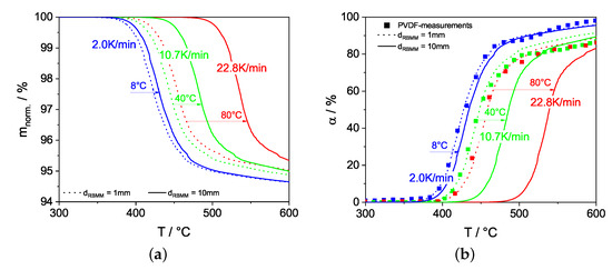
Figure 9.
Calculation results from the sRBMM with the diameters mm and mm at the heating rates 2.0 K/min, 10.7 K/min, and 22.8 K/min for investigation of scaling dependence on the applied heating in thermal treatment. (a) Normalized mass . (b) Extent of conversion .
Figure 9b displays the extent of conversion of the binder PVDF over the temperature. To compare the calculated degradation of the binder PVDF with the measurements, the TGA measurements are plotted as squares in this graph. The colors of the squares correspond to the heating rate .
The PVDF measurements are accurately predicted by the scaling with a diameter mm, while the calculations for the diameter mm show a temperature delay, which does not represent the current case. For larger particle diameters than 1 mm and higher heating rates, there is a delay in the degradation curve and a deviation from the measurement. This delay is due to the larger temperature difference between the particle and crucible, as shown in the following figures. Therefore, the scaling parameter is strongly dependent on the heating rate, which means that, to determine the maximum diameter of the RBMM particle, the heating rate of the particular thermal treatment case should be considered.
In addition, to evaluate the success of the thermal treatment, the extent of conversion of the binder is more significant, rather than the normalized mass . The normalized mass differs by only in all calculations, whereas the extent of conversion shows a difference of approximately . Additionally, the difference in the normalized mass becomes less significant as the initial weight fraction of the binder in the BM decreases, while the difference in the extent of conversion remains constant and comparable.
In Figure 10, the results of the calculated heat fluxes for the sRBMM are shown. Figure 10a shows the results for the smaller diameter, and Figure 10b shows the results for the larger diameter. In these plots, the heat flux for the heating rate K/min is shown in blue, for K/min in green, and for K/min in red. Furthermore, for the heating rate K/min, the heat transfer mechanisms are divided into EHT and radiation. Additionally, the ratio of EHT to radiation is the same for the smaller heating rates and for the same RBMM diameter.
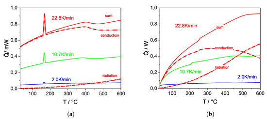
Figure 10.
Heat flux between the wall and the particle over the wall temperature T. Calculation results from the sRBMM at the heating rates 2.0 K/min, 10.7 K/min, and 22.8 K/min. (a) Diameter mm. (b) Diameter mm.
The black curves are the analytically calculated heat fluxes using the temperatures of the RBMM particle and the wall to validate the calculated heat fluxes with the DEM solver. These curves show also good agreement and validate the newly implemented radiation model in LIGGGHTS-PFM.
For the smaller RBMM diameter, EHT is more important than radiative heat transfer. For the larger RBMM particles, a different relationship between the heat transfer mechanisms is shown. As expected, at lower temperatures, the EHT is more pronounced than the radiation, and at higher temperatures, the radiation reaches the same amount of heat flux as the EHT for this case. Increasing the diameter of the RBMM by a factor of 10 results in a 1000-fold increase in the total heat capacity (=), while the projected heat transfer area within the bulk material only increases by a factor of 10 and the projected heat transfer area by radiation increases by a factor of 100. These scaling effects lead to a lower ratio of heat transfer area to heat capacity for larger RBMM particles. These results demonstrate the expected behavior of the RBMM particle model. A larger RBMM diameter includes and homogenizes more BM particles in the representative volume, resulting in a greater mass and smaller heat transfer area. Additionally, a larger RBMM particle volume leads to the larger spatial averaging of this representative volume due to larger discretization in space and can be compensated for by the respective effective heat transfer parameters associated with the particular case.
Figure 10 shows that, for smaller diameters, peaks can be observed at the defined melting temperature at around 165 °C. For the larger RBMM diameter, the melting temperature occurs later and the peaks are more characterized as a jump in the heat flux . The second effect is that the heat flux increases with temperature in all curves until binder degradation begins. After this event, the heat flux changes its slope. The increase in heat flux is due to the increase in the specific heat capacity of the RBMM particle with temperature. This means that more heat is required to heat the RBMM particle. Mass loss occurs as the binder in the RBMM particle degrades. This results in less heat being required to increase the temperature of the RBMM particle, leading to this change in slope. This also demonstrates a marker for the loss of representativeness.
In Figure 11, the temperature difference between the RBMM particles and the wall temperature over time is shown. Figure 11a shows the temperature difference of the smaller diameter and Figure 11b shows the temperature difference of the larger diameter. Comparing these plots, it can be observed that the temperature difference is smaller for the smaller RBMM diameter compared to the large diameter. For the smaller RBMM diameter, the smaller temperature difference indicates that the RBMM temperature is close to the defined wall temperature , which explains the well-predicted extent of conversion . Figure 11b shows the greater temperature differences resulting in the delay in binder degradation in Figure 9a,b.
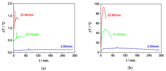
Figure 11.
Temperature difference between the wall temperature and the particle temperature over time. Calculation results from the sRBMM at the heating rates 2.0 K/min, 10.7 K/min, and 22.8 K/min (a) Diameter mm. (b) Diameter mm.
Figure 12 and Figure 13 show the heat fluxes into the RBMM particle over time for the six calculations, examining also the enthalpy of fusion . Figure 12 shows the heat fluxes for the smaller diameter and Figure 13 shows the heat fluxes for the larger diameter. The color blue corresponds to the heating rate K/min, green to K/min, and red to K/min. Each peak is also analyzed and its maximum and width are shown in the graphs, where the rotated numbers are the time in seconds for the start, maximum, and end of the peak. The summarized results of the analysis of the peaks are given in Table 7.
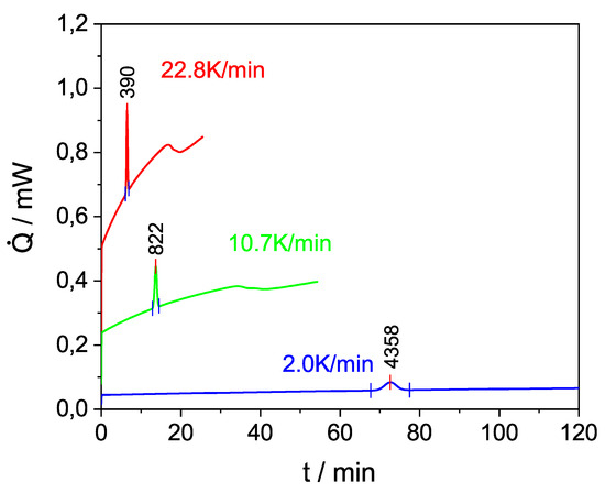
Figure 12.
Heat flux into the RBMM particle with diameter mm over the time. Calculation results from the sRBMM at the heating rates 2.0 K/min, 10.7 K/min, and 22.8 K/min.
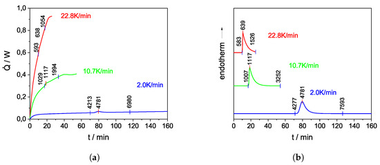
Figure 13.
Heat flux into the RBMM particle with diameter mm over the time. Calculation results from the sRBMM at the heating rates 2.0 K/min, 10.7 K/min, and 22.8 K/min. (a) Without knowledge of exact baseline. (b) With exact baseline.
Table 7.
Peak analysis of the heat flux into the RBMM particle.
In this table, the analyzed peak temperature, the amount of heat for the peak area, and the heat of fusion , related to PVDF, are listed. For the smaller diameter , the peak temperatures agree very well with the defined melting temperature of 165 °C and increase slightly with higher heating rates. For the larger diameter , this effect can also be observed, but with a greater lag to the melting temperature. These differences in melting temperature correspond to the peaks in the temperature difference shown in Figure 11. By measuring the amount of heat for each peak, it is found that the peak area for the smaller RBMM diameter is approximately 5.3 mJ for all heating rates, and converting this amount of heat into the corresponding binder of leads to the defined heat of fusion of the binder PVDF of 40 kJ/kg.
The analysis of the peaks for the larger RBMM diameters without referring to the baseline is shown in Figure 13a. It appears that this results in a lower heat of fusion as the heating rate increases. This is because of the superposition of two effects. The first effect is the higher ratio of inert mass to heat transfer area, which leads to a larger temperature difference compared to the smaller RBMM diameter (see Figure 11). This leads to a larger temperature change for the larger RBMM diameter , which is reflected in a broader peak. The second effect is that the slope of the heat flux changes the mass loss due to binder degradation. When these two effects occur simultaneously, a reduced peak area is calculated, resulting in an apparently reduced heat of fusion . This reduced heat of fusion is given in brackets in Table 7, which lists the peaks without knowledge of the exact baseline. By repeating the calculations with the larger diameter and without considering the heat of fusion for the binder, the baseline is obtained. By correcting the results shown in Figure 13a, the correct peak can be analyzed, as shown in Figure 13b. Comparing these two peaks, it can be seen that the start and maximum of the same peaks give similar results regardless of whether the baseline is known. However, comparing the end time of the peaks reveals a superposition effect. By evaluating these peaks, the expected heat of fusion of about 40 kJ/kg is calculated, as listed in the table.
4. Conclusions
Here, a Representative Black Mass Model (RBMM) is developed based on varying BM compositions and a coarse-graining approach in a DEM environment. By coupling isoconversional kinetics (OFW method) with DEM and implementing radiative heat transfer between particles and walls in LIGGGHTS-PFM, along with a coarse-graining approach proposed by Bierwisch et al. [29], it becomes possible to simulate the thermal treatment of black mass obtained from spent LIBs, taking into account the degradation of polymer-based binders.
This approach enables the simulation and monitoring of binder degradation at the level of BM particles throughout the entire physical treatment duration. The developed model framework is applied to an artificial but representative BM composition, utilizing kinetic data for the binder PVDF obtained from TGA measurements and applied to the Specific RBMM (sRBMM), where catalytic reactions are not considered. Additionally, the model allows the analysis of sample size effects in TG measurements, which is generally an important issue in TGA measurements (Zimmermann et al. [48]) and could be applied in this context in the future for different specific black mass compositions. Additionally, degradation simulations are carried out with two different RBMM particle sizes and various heating rates to examine the relationship between the scaling factor and the heating rate in a quasi-resting BM system. The results indicate that at low heating rates (2 K/min), the particle size can be increased to 10 mm for the studied BM without a significant impact on the conversion. However, this changes when the heating rate increases by about an order of magnitude to approximately 22 K/min. At this point, the diameter must be reduced by approximately one order of magnitude to 1 mm while still matching the experimental conversion data. These findings demonstrate a strong relationship between the scaling factor and the heating rate. Nevertheless, until the diameter reaches 1 mm, the influence of the heating rate is not significant, allowing for accurate predictions.
Furthermore, the required heat consumption for the particular BM to degrade the binder was calculated. Using this framework and the analyzed BM in conjunction with the scaling factor, future studies can focus on investigating BM binder degradation in specific apparatuses.
Author Contributions
Conceptualization, C.N., M.M. and M.F.; methodology, C.N., M.M. and M.F.; software, C.N.; validation, C.N., M.M. and M.F.; formal analysis, C.N., M.M. and M.F.; investigation, C.N., M.M. and M.F.; resources, C.N., M.M. and M.F.; data curation, C.N.; writing—original draft preparation, C.N., M.M. and M.F.; writing—review and editing, C.N., M.M. and M.F.; visualization, C.N., M.M. and M.F.; supervision, C.N., M.M. and M.F.; project administration, C.N., M.M. and M.F.; funding acquisition, M.M. and M.F. All authors have read and agreed to the published version of the manuscript.
Funding
This research was funded by the German Federal Ministry of Education and Research, grant number 03XP0354E.
Institutional Review Board Statement
Not applicable.
Data Availability Statement
The data presented in this study are available on request from the corresponding author.
Acknowledgments
The project on which this publication is based was funded by the German Federal Ministry of Education and Research within the Competence Cluster Recycling & Green Battery (greenBatt) under grant number 03XP0354E. The authors are responsible for the contents of this publication. We acknowledge support by the Open Access Publishing Fund of Clausthal University of Technology. We also express our appreciation and gratitude to Dennis Yutani for the English proof reading.
Conflicts of Interest
The authors declare no conflicts of interest. The funders had no role in the design of the study; in the collection, analyses, or interpretation of data; in the writing of the manuscript; or in the decision to publish the results.
Abbreviations
The following abbreviations are used in this manuscript:
| BM | Black mass |
| BC | Boundary condition |
| CAD | Computer-aided design |
| CMC | Carboxymethyl cellulose |
| DEM | Discrete element method |
| DSC | Difference scanning calorimetry |
| EHT | Effective heat transfer |
| HF | Hydrogen fluoride |
| HR | Heating rate |
| IC | Initial condition |
| LMO | Lithium metal oxide |
| NMC | Nickel manganese cobalt (the metals in the LMO) |
| OFW | Ozawa–Flynn–Wall |
| PVDF | Polyvinylidene fluoride |
| RBMM | Representative Black Mass Model |
| SBR | Styrene butadiene rubber |
| sRBMM | Specific Representative Black Mass Model |
| TGA | Thermogravimetric analysis |
References
- Bürklin, B.; Latz, T.; Schenk, L.; Degen, F.; Diehl, M.; Krätzig, O.; Paulsen, T.; Kampker, A.; Lackner, N.; Neef, C.; et al. Umfeldbericht zum Europäischen Innovationssystem Batterie 2022; Fraunhofer ISI: Karlsruhe, Germany, 2022. [Google Scholar]
- Grohol, M.; Veeh, C. Study on the Critical Raw Materials for the EU 2023: Final Report; Publications Office of the European Union: Luxembourg, 2023. [Google Scholar] [CrossRef]
- Mossali, E.; Picone, N.; Gentilini, L.; Rodrìguez, O.; Pérez, J.M.; Colledani, M. Lithium-ion batteries towards circular economy: A literature review of opportunities and issues of recycling treatments. J. Environ. Manag. 2020, 264, 110500. [Google Scholar] [CrossRef]
- Li, H.; Qiu, H.; Schirmer, T.; Goldmann, D.; Fischlschweiger, M. Tailoring Lithium Aluminate Phases Based on Thermodynamics for an Increased Recycling Efficiency of Li-Ion Batteries. ACS EST Eng. 2022, 2, 1883–1895. [Google Scholar] [CrossRef]
- Li, H.; Ranneberg, M.; Fischlschweiger, M. High-Temperature Phase Behavior of Li2O-MnO with a Focus on the Liquid-to-Solid Transition. JOM 2023, 75, 5796–5807. [Google Scholar] [CrossRef]
- Babanejad, S.; Ahmed, H.; Andersson, C.; Samuelsson, C.; Lennartsson, A.; Hall, B.; Arnerlöf, L. High-Temperature Behavior of Spent Li-Ion Battery Black Mass in Inert Atmosphere. J. Sustain. Metall. 2022, 8, 566–581. [Google Scholar] [CrossRef]
- Vanderbruggen, A.; Hayagan, N.; Bachmann, K.; Ferreira, A.; Werner, D.; Horn, D.; Peuker, U.; Serna-Guerrero, R.; Rudolph, M. Lithium-Ion Battery Recycling- Influence of Recycling Processes on Component Liberation and Flotation Separation Efficiency. ACS EST Eng. 2022, 2, 2130–2141. [Google Scholar] [CrossRef]
- Lombardo, G.; Ebin, B.; Steenari, B.M.; Alemrajabi, M.; Karlsson, I.; Petranikova, M. Comparison of the effects of incineration, vacuum pyrolysis and dynamic pyrolysis on the composition of NMC-lithium battery cathode-material production scraps and separation of the current collector. Resour. Conserv. Recycl. 2021, 164, 105142. [Google Scholar] [CrossRef]
- Nagl, R.; Fan, Z.; Nobis, C.; Kiefer, C.; Fischer, A.; Zhang, T.; Zeiner, T.; Fischlschweiger, M. Study of isobaric vapor–liquid equilibria of diethyl carbonate + ethylene carbonate for lithium-ion battery electrolyte solvent recycling. J. Mol. Liq. 2023, 386, 122449. [Google Scholar] [CrossRef]
- Abdollahifar, M.; Doose, S.; Cavers, H.; Kwade, A. Graphite Recycling from End–of–Life Lithium–Ion Batteries: Processes and Applications. Adv. Mater. Technol. 2023, 8, 2200368. [Google Scholar] [CrossRef]
- Petranikova, M.; Naharro, P.L.; Vieceli, N.; Lombardo, G.; Ebin, B. Recovery of critical metals from EV batteries via thermal treatment and leaching with sulphuric acid at ambient temperature. Waste Manag. 2022, 140, 164–172. [Google Scholar] [CrossRef]
- Huang, Z.; Liu, X.; Zheng, Y.; Wang, Q.; Liu, J.; Xu, S. Boosting efficient and low-energy solid phase regeneration for single crystal LiNi0.6Co0.2Mn0.2O2 via highly selective leaching and its industrial application. Chem. Eng. J. 2023, 451, 139039. [Google Scholar] [CrossRef]
- Liu, X.; Wang, R.; Liu, S.; Pu, J.; Xie, H.; Wu, M.; Liu, D.; Li, Y.; Liu, J. Organic Eutectic Salts–Assisted Direct Lithium Regeneration for Extremely Low State of Health Ni–Rich Cathodes. Adv. Energy Mater. 2023, 13, 2302987. [Google Scholar] [CrossRef]
- Werner, D.; Peuker, U.A.; Mütze, T. Recycling Chain for Spent Lithium-Ion Batteries. Metals 2020, 10, 316. [Google Scholar] [CrossRef]
- Mousa, E.; Hu, X.; Ånnhagen, L.; Ye, G.; Cornelio, A.; Fahimi, A.; Bontempi, E.; Frontera, P.; Badenhorst, C.; Santos, A.C.; et al. Characterization and Thermal Treatment of the Black Mass from Spent Lithium-Ion Batteries. Sustainability 2023, 15, 15. [Google Scholar] [CrossRef]
- Xiao, J.; Li, J.; Xu, Z. Recycling metals from lithium ion battery by mechanical separation and vacuum metallurgy. J. Hazard. Mater. 2017, 338, 124–131. [Google Scholar] [CrossRef] [PubMed]
- Lombardo, G.; Ebin, B.; St. J. Foreman, M.R.; Steenari, B.M.; Petranikova, M. Chemical Transformations in Li-Ion Battery Electrode Materials by Carbothermic Reduction. ACS Sustain. Chem. Eng. 2019, 7, 13668–13679. [Google Scholar] [CrossRef]
- Lombardo, G.; Ebin, B.; St J Foreman, M.R.; Steenari, B.M.; Petranikova, M. Incineration of EV Lithium-ion batteries as a pretreatment for recycling—Determination of the potential formation of hazardous by-products and effects on metal compounds. J. Hazard. Mater. 2020, 393, 122372. [Google Scholar] [CrossRef]
- Vyazovkin, S.; Burnham, A.K.; Criado, J.M.; Pérez-Maqueda, L.A.; Popescu, C.; Sbirrazzuoli, N. ICTAC Kinetics Committee recommendations for performing kinetic computations on thermal analysis data. Thermochim. Acta 2011, 520, 1–19. [Google Scholar] [CrossRef]
- Vanderbruggen, A.; Gugala, E.; Blannin, R.; Bachmann, K.; Serna-Guerrero, R.; Rudolph, M. Automated mineralogy as a novel approach for the compositional and textural characterization of spent lithium-ion batteries. Miner. Eng. 2021, 169, 106924. [Google Scholar] [CrossRef]
- Friedman, H.L. Kinetics of thermal degradation of char–forming plastics from thermogravimetry. Application to a phenolic plastic. J. Polym. Sci. Part C Polym. Symp. 1964, 6, 183–195. [Google Scholar] [CrossRef]
- Ozawa, T. A New Method of Analyzing Thermogravimetric Data. Bull. Chem. Soc. Jpn. 1965, 38, 1881–1886. [Google Scholar] [CrossRef]
- Flynn, J.H.; Wall, L.A. A quick, direct method for the determination of activation energy from thermogravimetric data. J. Polym. Sci. Part B Polym. Lett. 1966, 4, 323–328. [Google Scholar] [CrossRef]
- Akahira, T.; Sunose, T. Method of determining activation deterioration constant of electrical insulating materials. Res. Rep. Chiba Inst. Technol. (Sci. Technol.) 1971, 16, 22–31. [Google Scholar]
- Vyazovkin, S.; Dollimore, D. Linear and Nonlinear Procedures in Isoconversional Computations of the Activation Energy of Nonisothermal Reactions in Solids. J. Chem. Inf. Comput. Sci. 1996, 36, 42–45. [Google Scholar] [CrossRef]
- Vyazovkin, S. Evaluation of activation energy of thermally stimulated solid-state reactions under arbitrary variation of temperature. J. Comput. Chem. 1997, 18, 393–402. [Google Scholar] [CrossRef]
- Vyazovkin, S. Modification of the integral isoconversional method to account for variation in the activation energy. J. Comput. Chem. 2001, 22, 178–183. [Google Scholar] [CrossRef]
- Yeom, S.B.; Ha, E.S.; Kim, M.S.; Jeong, S.H.; Hwang, S.J.; Du Choi, H. Application of the Discrete Element Method for Manufacturing Process Simulation in the Pharmaceutical Industry. Pharmaceutics 2019, 11, 414. [Google Scholar] [CrossRef] [PubMed]
- Bierwisch, C.; Kraft, T.; Riedel, H.; Moseler, M. Three-dimensional discrete element models for the granular statics and dynamics of powders in cavity filling. J. Mech. Phys. Solids 2009, 57, 10–31. [Google Scholar] [CrossRef]
- Poly(Vinylidenfluorid) Average Mw ∼534,000 by GPC, Powder | Sigma-Aldrich. 19 September 2023. Available online: https://export.vwr.com/store/product/25409981/poly-vinylidene-fluoride-m-w-534-000-by-gpc-powder-sigma-aldrich (accessed on 31 December 2023).
- GitHub. ParticulateFlow/LIGGGHTS-PFM: This Is an Academic Adaptation of the LIGGGHTS Software Package, Released by the Department of Particulate Flow Modelling at Johannes Kepler University in Linz, Austria. Available online: http://www.jku.at/pfm (accessed on 20 November 2023).
- Chaudhuri, B.; Muzzio, F.J.; Tomassone, M.S. Modeling of heat transfer in granular flow in rotating vessels. Chem. Eng. Sci. 2006, 61, 6348–6360. [Google Scholar] [CrossRef]
- Department of Particulate Flow Modelling. LIGGGHTS Documentation, Release 21.11. Ph.D. Thesis, Johannes Kepler University Linz, Linz, Austria, 2022. [Google Scholar]
- Bouzennada, T.; Mechighel, F.; Filali, A.; Ghachem, K.; Kolsi, L. Numerical investigation of heat transfer and melting process in a PCM capsule: Effects of inner tube position and Stefan number. Case Stud. Therm. Eng. 2021, 27, 101306. [Google Scholar] [CrossRef]
- Xu, Z.X.; Zhang, C.X.; He, Z.X.; Wang, Q. Pyrolysis Characteristic and kinetics of Polyvinylidene fluoride with and without Pine Sawdust. J. Anal. Appl. Pyrolysis 2017, 123, 402–408. [Google Scholar] [CrossRef]
- Meireles, N. Separation of Anode from Cathode Material from End of Life Li-Ion Batteries (LIBs). Master’s Thesis, Luleå University of Technology, Luleå, Sweden, 2020. [Google Scholar]
- Schreiner, D.; Lindenblatt, J.; Daub, R.; Reinhart, G. Simulation of the Calendering Process of NMC–622 Cathodes for Lithium–Ion Batteries. Energy Technol. 2023, 11, 2200442. [Google Scholar] [CrossRef]
- Richter, F.; Kjelstrup, S.; Vie, P.J.; Burheim, O.S. Thermal conductivity and internal temperature profiles of Li-ion secondary batteries. J. Power Sources 2017, 359, 592–600. [Google Scholar] [CrossRef]
- Mohanty, D.; Hockaday, E.; Li, J.; Hensley, D.K.; Daniel, C.; Wood, D.L. Effect of electrode manufacturing defects on electrochemical performance of lithium-ion batteries: Cognizance of the battery failure sources. J. Power Sources 2016, 312, 70–79. [Google Scholar] [CrossRef]
- Ho, H.; Cheung, W.L.; Gibson, I. Effects of graphite powder on the laser sintering behaviour of polycarbonate. Rapid Prototyp. J. 2002, 8, 233–242. [Google Scholar] [CrossRef]
- Varma-Nair, M.; Wunderlich, B. Heat capacity and other thermodynamic properties of linear macromolecules X. Update of the ATHAS 1980 Data Bank. J. Phys. Chem. Ref. Data 1991, 20, 349–404. [Google Scholar] [CrossRef]
- Masoumi, M. Thermochemical and Electrochemical Investigations of Li(Ni,Mn,Co)O2 (NMC) as Positive Electrode Material for Lithium-Ion Batteries. Ph.D. Dissertation, Karlsruher Instituts für Technologie, Karlsruhe, Germany, 2019. [Google Scholar]
- Spencer, H.M. Empirical Heat Capacity Equations of Gases and Graphite. Ind. Eng. Chem. 1948, 40, 2152–2154. [Google Scholar] [CrossRef]
- Indolia, A.P.; Gaur, M.S. Investigation of structural and thermal characteristics of PVDF/ZnO nanocomposites. J. Therm. Anal. Calorim. 2013, 113, 821–830. [Google Scholar] [CrossRef]
- Sigma-Aldrich. Safety Data Sheet, Produktname: Poly(Vinylidene Fluoride), Produktnummer: 182702, CAS-Nr. 24937-79-9. 2021. Available online: https://www.vanderbilt.edu/vinse/facilities/safety_data_sheets/Poly_vinylidene_fluoride.pdf (accessed on 26 December 2023).
- Gotcu, P.; Pfleging, W.; Smyrek, P.; Seifert, H.J. Thermal behaviour of LixMeO2 (Me = Co or Ni + Mn + Co) cathode materials. Phys. Chem. Chem. Phys. PCCP 2017, 19, 11920–11930. [Google Scholar] [CrossRef] [PubMed]
- Adibekyan, A.; Kononogova, E.; Hameury, J.; Lauenstein, M.; Monte, C.; Hollandt, J. Emissivity measurements on reflective insulation materials. TM Tech. Mess. 2021, 88, 617–625. [Google Scholar] [CrossRef]
- Zimmermann, J.; Mansouri, S.; Nobis, C.; Irmer, M.; Beuermann, S.; Fischlschweiger, M. Influence of Molecular Characteristics and Size Effects in Polystyrene Pyrolysis. Chem. Ing. Tech. 2023, 95, 1339–1343. [Google Scholar] [CrossRef]


Disclaimer/Publisher’s Note: The statements, opinions and data contained in all publications are solely those of the individual author(s) and contributor(s) and not of MDPI and/or the editor(s). MDPI and/or the editor(s) disclaim responsibility for any injury to people or property resulting from any ideas, methods, instructions or products referred to in the content. |
© 2024 by the authors. Licensee MDPI, Basel, Switzerland. This article is an open access article distributed under the terms and conditions of the Creative Commons Attribution (CC BY) license (https://creativecommons.org/licenses/by/4.0/).